
Timeliness reduction on industrial turnover index based on machine learning algorithms
Abstract
The modernisation of the production of official statistics should make use not only of new data sources but also of novel statistical methods applied to traditional survey and administrative data. This improves the traditional quality standards. Here we present an application of statistical learning algorithms to improve the timeliness under a controlled compromise of accuracy of the Spanish Industrial Turnover Index (ITI). The methodology has been developed based on a modular and standardized approach that could be easily extended to other surveys. Our advanced index allows us to predict the ITI 31 days before publication with a median error of 0.5 points over the period Mar 2016–Apr 21, in an index with large oscillations. The results are promising and support the idea of the use of these techniques in improving the quality dimension of timeliness while accuracy is kept under control.
1.Introduction
Since the beginning of the 21st century, Official Statistics have faced a series of challenges related to pressing technological advances that require statistical modernization. This challenge has been present for over a decade now with the creation of the High-Level Group for the Modernisation of Official Statistics (HLGMOS) having great results [1]. However, this issue has become more relevant and urgent than ever in crisis situations such as the COVID-19 outbreak. This modernization must take place, according to the work of the UNECE, in several areas that support the Official Statistics and that are closely interrelated with each other: human resources, organizational frameworks and evaluation; the implementation of methods and new technologies in statistical production; data collection and data sources; dissemination and communication; standards and metadata [2].
These areas can be grouped into three basic pillars: (i) industrial standardization, (ii) new data sources, and (iii) new statistical methods. Industrial standardization involves the use of international production standard models such as the GSBPM (Generic Statistical Business Process Model) or the GSIM (Generic Statistical Information Model). One of the main aspects of these models is the implementation of a modular approach in statistical production [3].
The incorporation of new data sources implies the coexistence of traditional data collection methods together with administrative records and new digital data. This incorporation establishes a set of challenges whose solutions go through the adoption of new production frameworks and the development of new statistical methods [4].
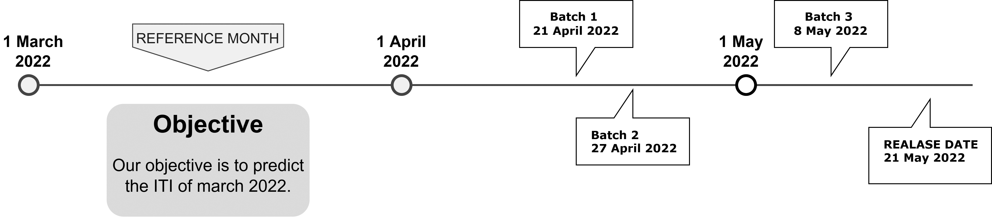
Figure 1.
Industrial Turnover Index’s timeline.
1.1New methods and technologies in statistical production: Machine learning
Machine Learning (ML) is a subset of artificial intelligence, which builds a mathematical model based on sample data, known as “training data”, to make predictions or decisions without being explicitly programmed to perform the task [5]. They consist of the design of statistical-computational models that, given some input data, extract information from these to estimate or predict an objective or output (supervised learning) or, simply, to analyze the different relationships that are established between those input data (unsupervised learning) [6].
The use of these techniques in Official Statistics is not yet widely extended, but they represent an innovation that can provide a solution to some of the major challenges that lie ahead [7]. In 2018, Statistics Germany (Destatis) conducted an in-depth analysis of the use of machine learning in official statistics. Most countries stated the use of machine learning, including Statistics Spain (INE)[8]. This study pointed out that most of the machine learning applications on the national statistical institutes (NSIs) are framed in the production phase of the GSBMP and are used for classification, imputation or linkage.
In this context, the traditional production phase of statistical data editing appears as a natural candidate for the modernisation of the whole production process and the improvement of several key quality dimensions such as timeliness, cost-efficiency, and accuracy. The General Statistical Data Editing Model (GSDEM) [9] provides a versatile, evolvable, and comprehensive production framework to design, implement, execute, and monitor so-called statistical data strategies, i.e. a collection of sequential and concurrent business functions to detect and treat non-sampling errors. In parallel, the use of machine learning techniques with this same goal has received due attention (see [8, 10] and multiple references therein) and highly relevant international projects are already producing important empirical results [11] (see especially theme 2 of work package 1 about edit and imputation).
• Accuracy vs Timeliness.
Nowadays immediacy is established in most aspects of life. Users require information, and the sooner the better. Nowcasting is defined as the prediction of the present, the very near future and the very recent past [12]. That is the reason why nowcasting methodologies such the one presented are getting attention in Official Statistics [13, 14]. Technological advances have led to the emergence of private producers of statistics that meet these needs and, in a way, compete with traditional institutions. Therefore, it is imperative that public statistical services invest part of their resources in improving timeliness but keeping an eye in the accuracy that characterizes them, to remain as reference producers of statistics [15].
• Measurement vs Prediction.
Although Machine Learning and new data sources improve the possibility of predicting, measuring is still the role and main objective of official statistical services. Therefore, an interesting application of ML techniques is to support the traditional measuring methods by helping in the treatment of missing values, in particular, and non-sampling errors, in general.
1.2Motivation
The main motivation of this work is to improve timeliness and relevance in the publication of official statistics by using machine learning imputation techniques at the microdata level. This is a very important quality dimension as is stated in the Trusted Smart Statistics[16] because, what could be considered timely and relevant before it is not necessarily acceptable in today’s datafied world. The usage of ML for imputation has been widely reported in the scientific literature in [17, 18, 19].
The goal is to provide an advanced industrial turnover index several weeks before the publication of the final index. Machine Learning techniques will allow to impute the missing values of the industrial turnover as the data arrives, reducing the burden on the respondent and speeding up the macro-editing. In this way, the ITI’s timeliness will be improved while maintaining high accuracy.
One of the advantages of machine learning compared to other statistical models like generalized linear models is the improvement in accuracy but at the expense of interpretability [20]. To edit data, interpretability is not the most relevant feature and therefore machine learning techniques will perform well.
ITI is part of the so called Short-term business statistics (STS). STSs are the earliest statistics released to show emerging trends in the European economy. Their relevance is reflected in the fact that 7 out of the 27 indicators included in the European Statistical Recovery Dashboard are STS indicators. The major advantage of the monthly and quarterly released STS data is that they are available very shortly after the end of the reference period. Nevertheless, during the Covid-19 pandemic, the NSIs were asked to improve the timeliness of these indicators in order to have faster data that could be useful for policy making. Inevitably this must be carried out searching for a trade-off between speed and accuracy.
The work is organized as follows. In Section 1.3 we describe the traditional production process of the ITI at Statistics Spain (INE) and briefly discuss about the concepts of advanced indices. In Section 2 we present the statistical methodology to compute the early estimates and describe the production process for the advanced index executed in the pilot study. In Section 3 we present the results for the periods between March 2016 to April 2021 and analyse them. Finally, in Section 4 we include some findings, limitations and future possibilities in this field of study.
1.3Industrial Turnover Index (ITI): Statistical process
The objective of Industrial Turnover Index is to measure the evolution of the activity of the companies that form part of the industrial sector in Spain, based on their turnover [21].
The results are presented in the form of indexes since the objective is to measure the turnover variation. The statistical unit is the establishment, which does not necessarily coincide with the company, so there are identification variables for both the company and the establishment for each reporting unit.
ITI is published 51 days after the end of the reference month. The data is collected in three batches. The first batch is collected 20 days after the end of the reference month and the response rate is 70–75%, The second batch is collected 27 days after the end of the month, and we get up to 80–85% and the third batch is collected 38 days after the end of the month, and we get 90–95%. According to the Spanish law, it is mandatory for respondents to send their responses, otherwise the sampling units can be fined.
The goal of this work is to build an Advanced ITI for each of the three batches and an initial estimation without any information from the reference month. Therefore, we will have the following advanced indexes.
• Advanced ITI 0: This advanced index is obtained when the previous month ITI is released, 20 days after the end of the month. It will not include any current month data. We will use this advanced index to see the effect of including current information in the other advanced indexes.
• Advanced ITI 1: This advanced index is obtained when the first batch is collected, 20 days after the end of the month.
• Advanced ITI 2: This advanced index is obtained when the second batch is collected, 27 days after the end of the month.
• Advanced ITI 3: This advanced index is obtained when the third batch is collected, 38 days after the end of the month.
All Advanced Indexes are computed using formulas described in the Section 2.
1.3.1Data collection
The data collection is carried out by regional delegations with a monthly survey.
There are different official classifications to get the disaggregation levels for the index, namely the geographical level (NUTS-2), the destination of the produced goods (Main Industrial Grouping – MIGs) and the Spanish adaptation of Statistical Classification of Economic Activities (NACE-2) which is called CNAE.
The sample comprises around 12000 units selected by cutoff sampling by NACE and NUTS2. The data is then sent to the headquarters to make the required processing to compute the indexes. Before being sent to the headquarters a first process of interactive data editing is carried out by the regional delegations but most of the editing and imputation process is done in the central services.
1.3.2Computing indexes
The first step to compute the final indexes is to get the elementary ones, which are those at the lowest possible level of aggregation. In the case of ITI those are computed for the intersection between NUTS-2 and NACE at 2 digits.
(1)
Where:
As we can see in Eq. (1), it is compulsory to have the information about the establishment in moth
To preserve statistical disclosure control, this indexes are not made public, and they are used only to compute the compound indexes. For computing those indexes, the weights for the aggregations are obtained through the Structural Business Statistics of the Industrial Sector as follows [22]:
(2)
Finally, the ITI is computed using a weighted average as follows:
(3)
Where:
Our advanced index proposal is based on Eqs (1) and (3) but computing advanced elementary index by using machine learning imputations.
(4)
Where:
Once the advanced elementary indexes are calculated, the derivation of the advanced composite index,
(5)
Finally, the index is seasonally adjusted following INE Spain standards.
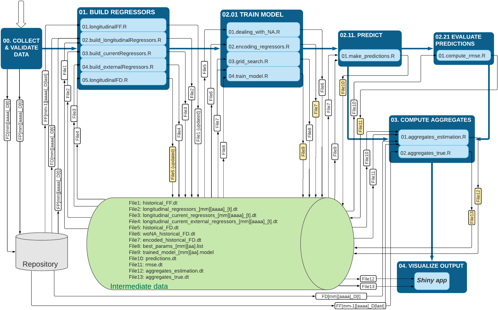
Figure 2.
Execution pipelines.
1.4Pipeline of the process and modularity
The production process for the early estimates of the ITI has been designed by following the international production standard models and the approach about the use of functional modularity stated in the working paper by Esteban et al. [3] with the aim of producing an industrialised standardized production process. The whole process is completely modular, consisting in several steps. The workflow and the flow of data can be observed in Fig. 2.
It consists of four main stages and a preliminary stage.
0. Preliminary stage: Collect and Validate Data.
1. Build Regressors: Regressors of the model are built from the data source files.
2. Train Model: Model is trained after some previous treatments related to dealing with the missing values, encode regressors and grid search.
3. Predict and Evaluate Predictions: Evaluation metrics are derived.
4. Compute Aggregates:Aggregates are computed using the estimations of the models and they are compared with the true aggregates to evaluate the global performance of the model.
5. Visualize Output: Results are shown in a R Shiny app.
The modularity approach can be observed in the fact that a general organization for the whole process exists, where each step is a folder and there are general data storage and functions that can be used in several steps. There is no survey-specific content, in the code implementation, only in the parameters files. For this reason, the scripts are valid for any survey. The source code for the whole process can be accessed at this repository (https://github.com/davidsalgado/AdvITI).
2.Methodology
In the current production process, we compute the population total
(6)
where
Notice that this can only be computed after finishing these two production phases (collection and editing). The goal is not to wait until all data collection and all data editing are concluded to produce an advanced estimation of the ITI with the ongoing collected information. Considering the values that we already know and predicting what we do not know yet, we decompose this estimate as follows:
(7)
Where
Based on this decomposition of the estimate and assuming
(8)
This estimator will be obtained applying machine learning methodology and algorithms that will be discussed below.
Table 1
Example of regressors matrix
| Norden | Date | Zip code | CNAE4_Code | CNO1FF | … |
|---|---|---|---|---|---|
| 00000001P | Jan15 | 28035 | 1234 | 1293451 | … |
| 00000001P | Feb15 | 28035 | 1234 | 854745 | … |
| … | … | … | … | … | … |
| 00000001P | Apr21 | 28035 | 1234 | 3293451 | … |
| 00000002P | Jan15 | 40400 | 8762 | 0 | … |
The predictor
(9)
We present here a modular approach used to calculate the estimator (8) using machine learning techniques. This estimator will be used to obtain an Advanced ITI. This approach can be generalized to many Short-Term Business Statistics.
Table 2
Typology of regressors
| ID | Cross | Long | Cross | External | |
|---|---|---|---|---|---|
| Hist. series |
|
|
|
|
|
| Running month |
|
|
|
|
|
• Prepare data. We gather raw data obtained by provincial services, and cleaned data edited and reviewed by central services. Cleaned data is obtained with a delay of 1 month. The data is collected from JAN-2015 to APR-2021. The data contains information of respondents and non respondents including their answers to the turnover survey and information about their activity, size, and location. We include an example of regressors matrix in Table 1.
Over these data we will use as target variable
• Build regressors. 187 regressors are derived from the data collected. We distinguish 5 types of them.
– ID variables: These variables contain direct information of the establishments and do not need to be processed, e.g., location or activity codes.
– Cross sectional variables: These variables are derived grouping rows by ID variables and calculating functions on those groups (means, quantiles, …), e.g., mean of the current turnover of the respondents by activity code. Note that cross sectional variables of the current month must be obtained from big size groups to avoid overfitting.
– Longitudinal variables: These variables are derived by summarizing the historical information of a given establishment, e.g., moving average of the previous 12 months. It is important to note that including current month information could lead to overfitting as most of the information of the non-respondents is not available during the running month.
– Cross sectional and longitudinal variables: These variables are derived grouping rows by ID variables and calculating longitudinal functions of these groups, e.g., annual rate of change in the turnover current mean grouped by activity.
– External variables. We include information from the industrial price index (IPRI) and industrial production index (IPI) that are available at
Figure 3.
Testing methodology.
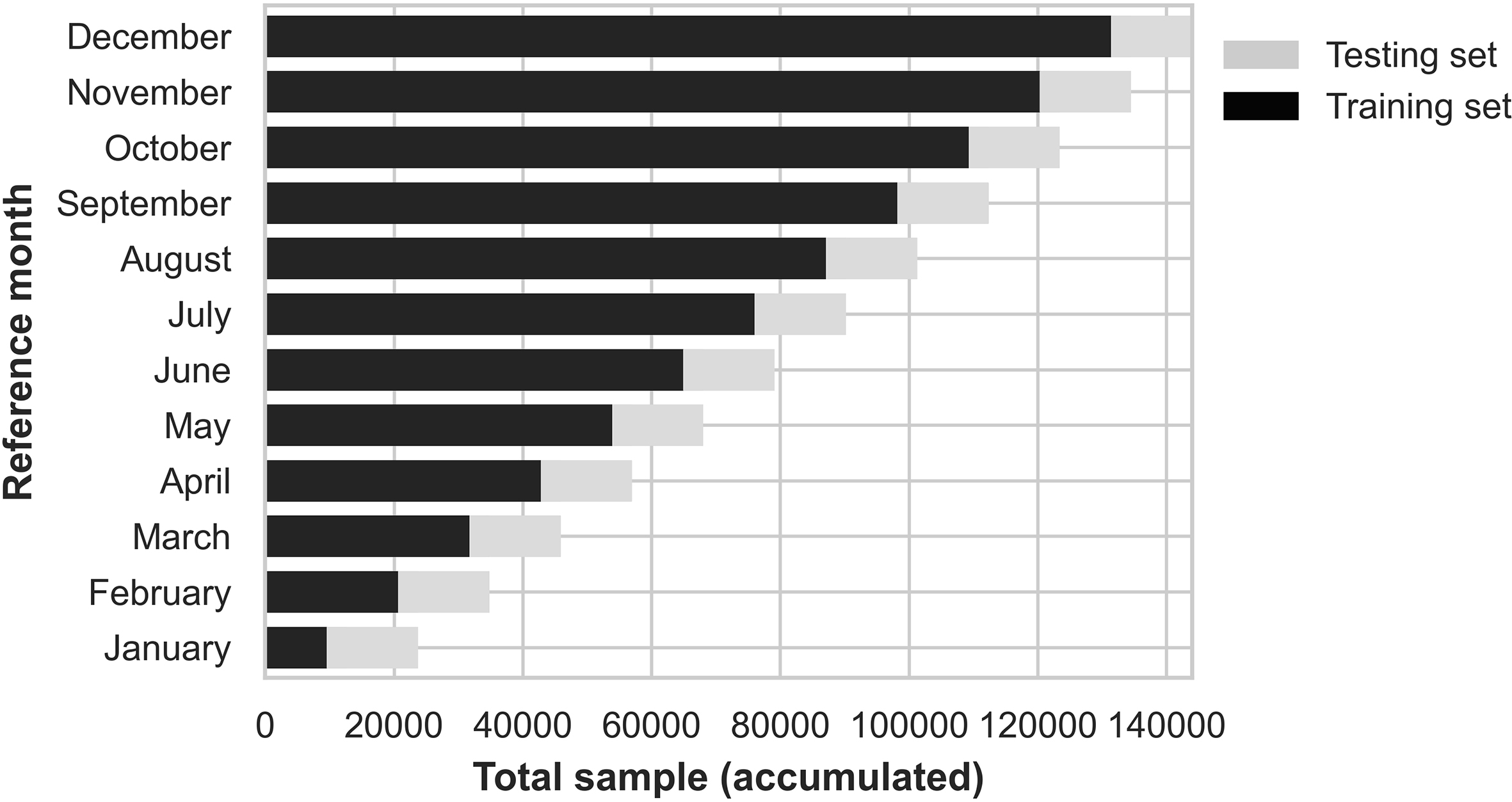
Figure 4.
General Advanced Industrial Turnover Index.
Regressors are calculated in two ways: using only historical data and including data from the current period. The typology of regressors is explained in Table 2. As it was stated in Section 1.3, we do not include any current data for the estimation of Advanced Index 0. The other three advanced indexes are estimated with historical data and available current data at the moment of their publication.
• Build model. The building model phase includes preprocessing, model selection, metric and loss function selection, grid search of hyperparameters and train final model.
– Pre-processing. We deal with missing values by imputing them using expert criteria rules. The categorical variables are encoded following two different strategies [23]:
* One-hot encoding for the categorical variables with few categories (
* Mean encoding for those with many categories.
– Model selection. We have used a boosting algorithm because we are concerned in low bias estimators. We are using lightgbm [24], an efficient implementation of traditional boosting techniques. Other algorithms preliminary tested were Lasso regression and random forest. The results obtained were worse, but a systematic analysis needs to be done.
– Minimize total error. The metric we desire to minimize is the total error, given by Eq. (9). This metric can not be used directly as a loss function for different reasons: it is only referred to a subset of the training set and it is not differentiable. It is important to note that this metric is mainly focused on favouring the reduction of bias over the reduction of variance, allowing big errors,
– Loss function selection. The loss function minimized during training is the Mean Squared Error (MSE),
(10)
we selected MSE for computability reasons and because this loss function is minimized in
(11)
where
Figure 5.
Feature importance.
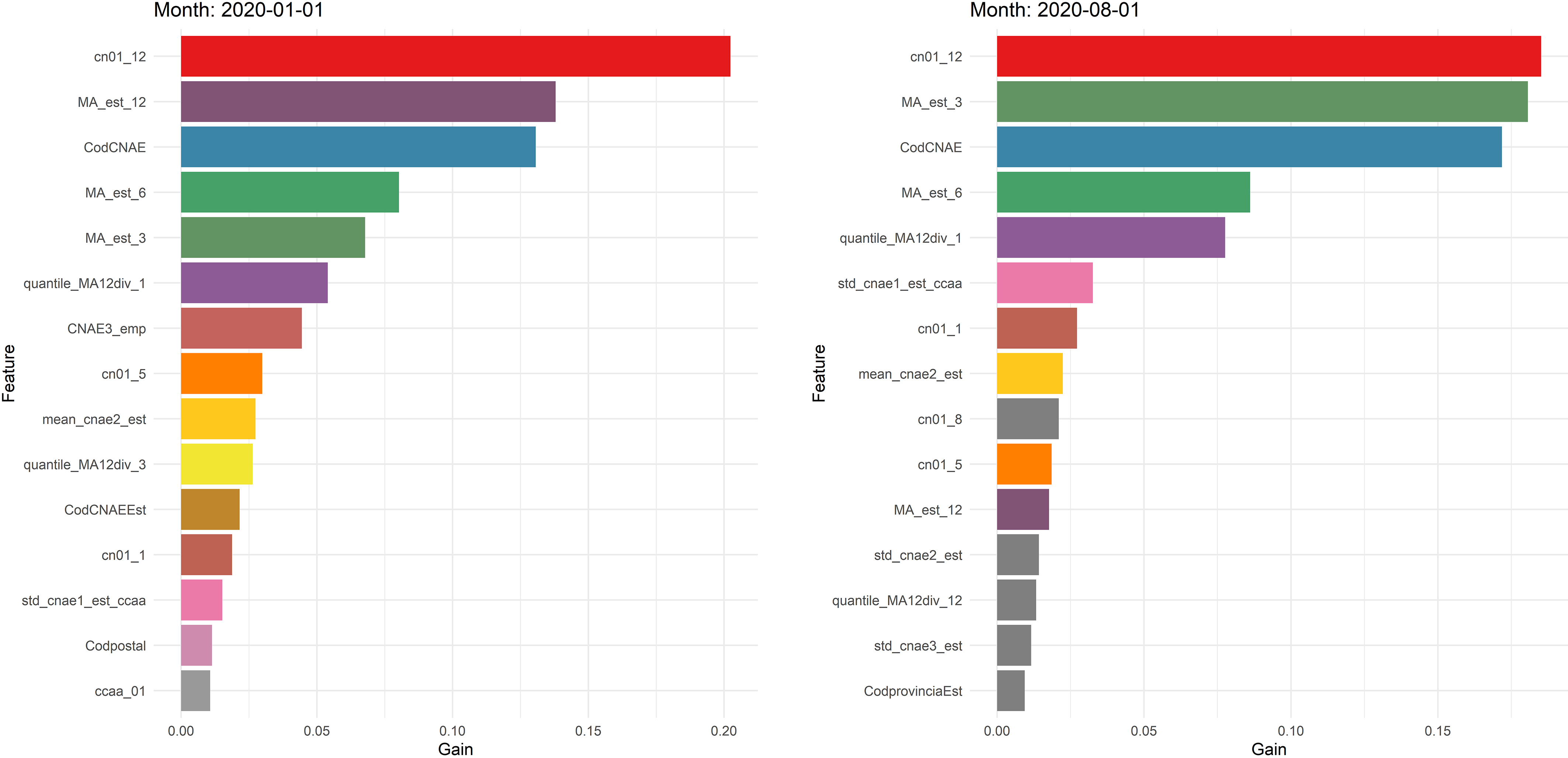
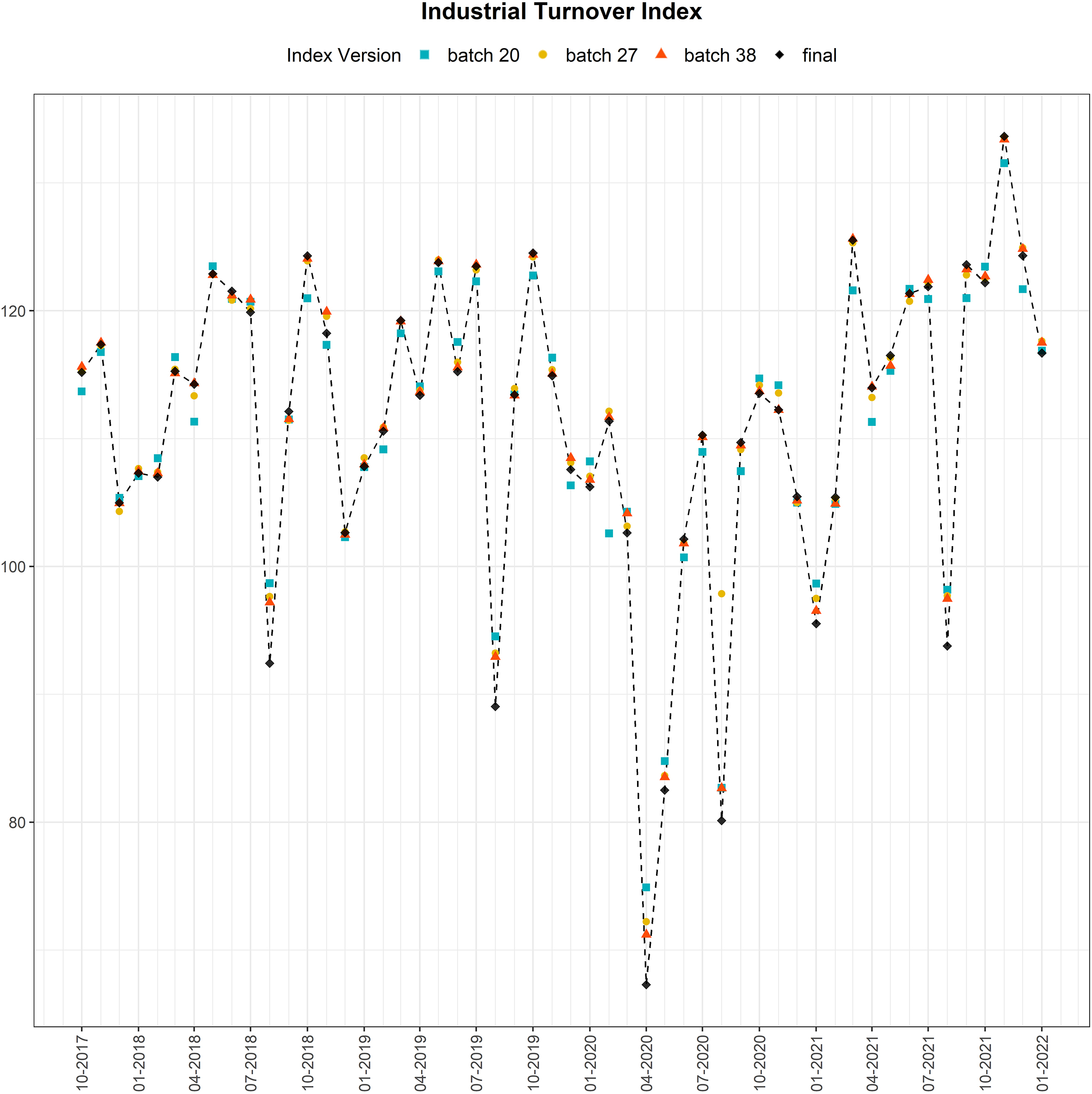
Figure 6.
General Advanced Industrial Turnover Index. The left panel corresponds to the first batch, the central panel to the second, and the right panel to the third and last batch. In blue, the Advanced ITI 0, which does not include current information; in black, the advanced ITI for each batch; in red, the final published index. For instance, in April 2020 our prediction for batch 01 (
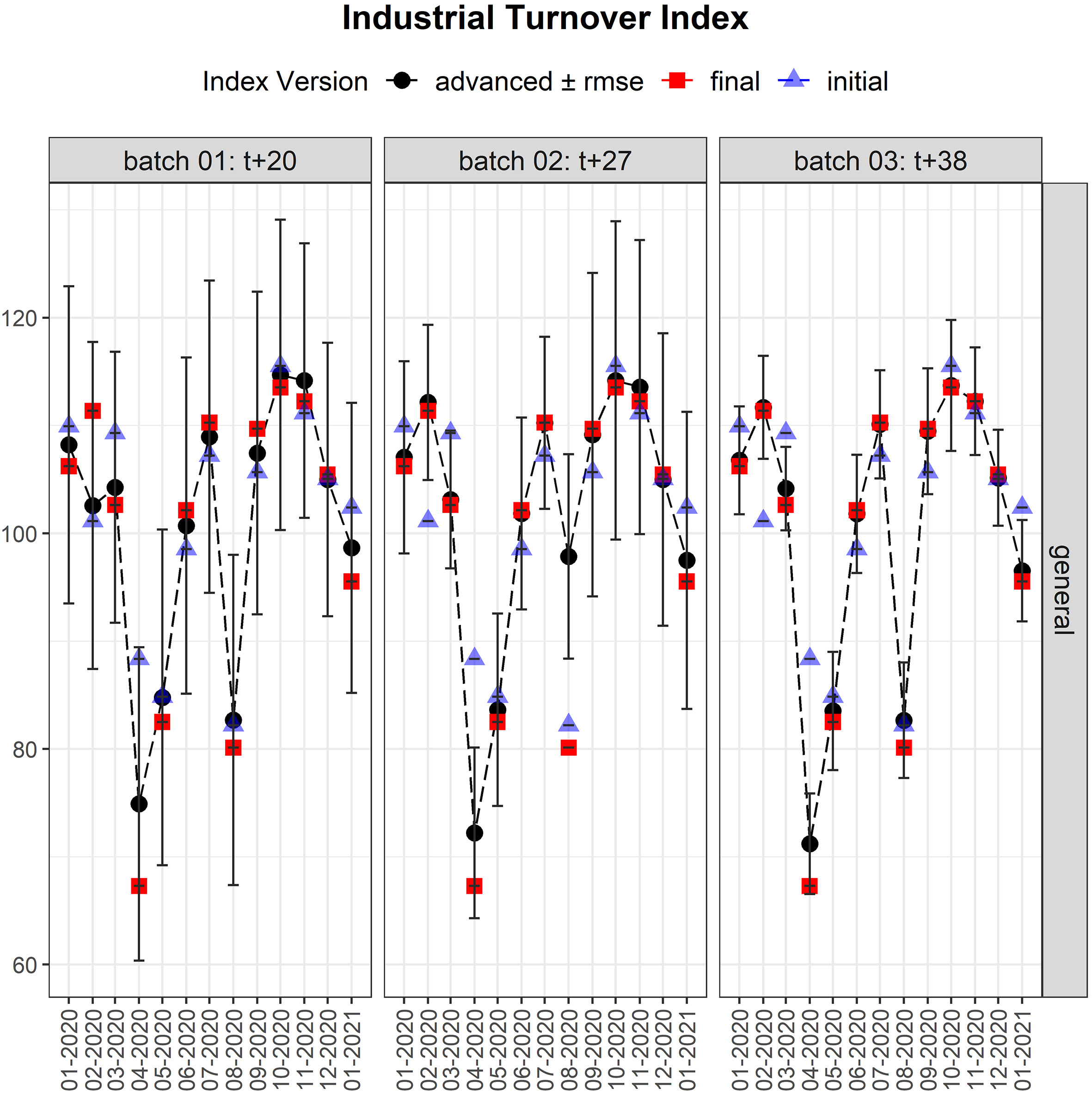
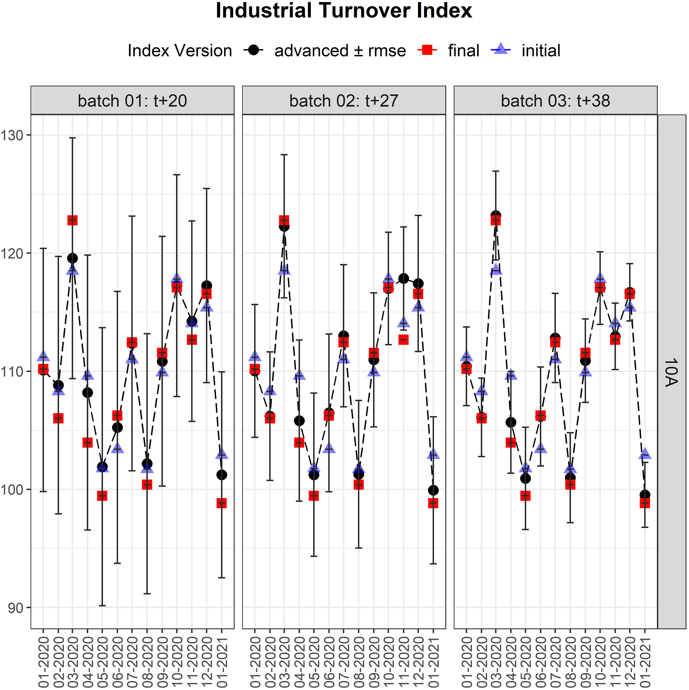
Figure 7.
General Advanced Industrial Turnover Index disaggregated by CNAE-09.
– Grid-search of hyperparameters. We do cross validation applied to time series by building models sequentially using the last month as test. We did an implementation in R following the idea in the TimeSeriesSplit function in “Scikit-learn” package [25]. The first model is trained with information from JAN2015–FEB2016 and validated in MAR16. We do this sequentially until the last model is trained with information from JAN2015–MAR2021 and validated in APR21. For each batch,
– Train final model. Once the loss function and best hyperparameters are selected, we train a different model for each month.
• Calculate Advanced Index. For each batch of the period MAR2016–APR2021 we predict the not-yet-collected values as follows: let the current month
3.Results
Firstly, we show the performance of the Advanced Industrial Turnover Index during the period March 2016–April 2021.
Advanced ITI is generally performing well. Performance increases with more available data as it is expected in a machine learning model. The model gets the seasonality but tends to overestimate August. In this month, the turnover becomes a semi-continuous variable, so in further development we will have to include a step to predict whether the value of the target variable is zero or different.
Figure 5 highlights the ability of the model to capture the seasonality, as the most relevant feature is the turnover of the establishment in the same month of the previous year (cn01_12).
Table 3
Metrics by batch
| Advanced Index 1 | Advanced Index 2 | Advanced Index 3 | |
|---|---|---|---|
| Mean absolute error | 1.808597 | 1.243692 | 0.8068145 |
| Median absolute error | 1.2073 | 0.52445 | 0.36475 |
One interesting result is the performance of the advanced ITI during the year 2020. In Fig. 6 we see the effect of the lockdown and how the Advanced ITI 0 is unable to predict April-20. The other advanced indexes, which include current month’s information, get the lockdown’s effect. This illustrates the importance of adding current periods data to the model.
In Feb-2020, there were some collection difficulties due to the lockdown (February was collected in April) so batch 01 was empty. Therefore, as we see in Fig. 6, the Advanced ITI 1 is the same as Advanced ITI 0.
One last consideration about that figure is that during August, one of the biggest industrial firms sent a huge erroneous turnover data in the batch 02 which led to a bad prediction of Advanced ITI 2. A previous light validation is needed to avoid this type of outliers.
The Advanced ITI can also be computed at different levels of disaggregation. For example, in Fig. 7, the Advanced Indexes are computed for the manufacture or food products. In that figure it is clearly seen how the initial prediction (ITI 0) gets generally improved by the data from the batch.
The following table shows the mean absolute error and median absolute error of the Advanced Indexes given by Eqs (12) and (13):
(12)
(13)
Where:
Table 3 shows that the error tends to be less than 1.2 points in batch 01, 0.5 points in batch 02 and 0.36 points in batch 03. It is important to note that the indexes are around 100, so these errors are around 1% of the index.
Mean Absolute Error is higher than Median Absolute Error due to mistakes during data collection, lockdown, and lack of accuracy in August among others. This issues, except August, are external to the model and, therefore, the median absolute error is a good proxy of the accuracy.
4.Conclusions
Advanced Industrial Turnover Indexes solve the problem of timeliness and at the same time maintain a good precision. Our proposal provides of an Advanced ITI close to the real index 31 days earlier. As the publication date draws nearer, more data is available, and the results converge to the real index.
Findings:
• Machine learning can help to reduce timeliness in short term business surveys, maintaining good accuracy levels. In addition, modularity makes the methodology applicable to other types of surveys.
• Our study shows that there is need of data from current period to obtain good estimates.
• Microdata, paradata and data from other surveys enrich the model.
• Outliers are very difficult to model and have an important effect on the model performance.
• It is specially useful when unexpected events occur, such as COVID-19 outbreak, because some features of the machine learning model include information of the rare event in the respondent units of the current month.
• Machine learning prediction models can be a great tool for the data editing and imputation team because they could compute and analyse discrepancies between real and predicted values. It is possible to receive erroneous values due to misreporting, misunderstandings or technical difficulties so with this methodology we can automatically detect them and warn the responsible.
Limitations of the study:
• The hyperparameter tuning process could be deeper if more computation power is available.
• The model is not very robust since most of the units are small or medium size, but a small proportion are big companies with a very important share of the total turnover of the division. This makes the prediction very volatile if the data of big firms is gathered or not. In this sense manual imputation is still a better choice for these units.
• The behavior of the turnover of some industrial sectors can be very difficult to predict since their turnover depends on few projects that can be reported in one month. For example naval or aerospace industry.
Future work:
• Data is available in 3 batches, however data is collected continuously so having daily data could increase the possibilities of the study.
• Apply to other kind of surveys. INE Spain is starting to evaluate this methodology for the national health survey and Economically Active Population Survey.
• Use machine learning to perform selective editing for determining the important and non important units.
• Use different machine learning models, such as, Neural Networks or Random Forests and ensemble learning.
• Select units that where imputed by traditional methods where the unit sent their data after the imputation. Then, apply our model to compare the performance of actual methodology against machine learning methodology.
This project was a pilot test for internal research about the feasibility of machine learning techniques to reduce timeliness in short term business statistics. The results of this pilot are not conceived to be published as statistical outputs because further development is needed to implement this methodology in production. However, we believe that this first steps are crucial to begin using machine learning in production of official statistics.
Acknowledgments
The authors are grateful to the whole Methodology Department of INE Spain and specially to David Salgado, Elena Rosa-Perez and Sandra Barragán. Their critical and constructive remarks, continuous guidance and help has made possible the present paper. The views expressed in this paper are those of the authors and do not necessary represent the official position of INE Spain.
References
[1] | Gjaltema T. High-Level Group for the Modernisation of Official Statistics (HLG-MOS) of the United Nations Economic Commission for Europe. Statistical Journal of the IAOS. Preprint: 1–6. |
[2] | UNECE. Modernization of official statistics. (2021) ; Available from http://unece.org/statistics/modernization-official-statistics. |
[3] | Esteban E, Novás M, Saldaña S, Salgado D, Sanguiao L. Data organisation and process design based on functional modularity for a standard production process. (2018) . |
[4] | Salgado D, Oancea B. On new data sources for the production of official statistics. arXiv:2023.06797v1, (2020) . |
[5] | Zhang XD. A matrix algebra approach to artificial intelligence. Springer; (2020) . |
[6] | Mohri M, Rostamizadeh A, Talwalkar A. Foundations of machine learning. MIT press; (2018) . |
[7] | Jahani E, Sundsøy P, Bjelland J, Bengtsson L, Pentland A, de Montjoye YA. mproving official statistics in emerging markets using machine learning and mobile phone data. EPJ Data Science. (2017) ; 6: : 1–21. |
[8] | Beck M, Dumpert F, Feuerhake J. Machine Learning in Official Statistics. arXiv:1812.10422, (2018) . |
[9] | UNECE. Generic Statistical Data Editing Model. (2021) ; Available from: https://statswiki.unece.org/display/sde/GSDEM. |
[10] | Puts M, Daas P. Machine Learning from the Perspective of Official Statistic. (2021) . |
[11] | UNECE, HLG-MOS Machine Learning Project (2022) ; Available from: http://unece.org/statistics/modernization-official-statistics. |
[12] | Giannone D, Reichlin L, Bańbura M, Modugno M. Now-casting and the real-time data flow. Working Paper Series 1564. European Central Bank; (2013) Jul. Available from: https://ideas.repec.org/p/ecb/ecbwps/20131564.html. |
[13] | European Statistics Awards for Nowcasting. Accessed: (2022) -10-07. Available from: https://statistics-awards.eu/. |
[14] | Koskimäki T, Luomaranta H. Experiences in the use of forecasting and nowcasting methods for official statistics. (2020) ; Available from: https://unstats.un.org/unsd/statcom/51st-session/side-events/documents/20200302-2L-Finland.pdf. |
[15] | Robin N, Klein T, Jütting J. Public-private partnerships for statistics: Lessons learned, future steps: A focus on the use of non-official data sources for national statistics and public policy. (2016) . |
[16] | Ricciato F, Wirthmann A, Giannakouris K, KlSkaliotisein M, et al. Trusted smart statistics: Motivations and principles. Statistical Journal of the IAOS. (2019) ; 35: (4): 589–603. |
[17] | Yung W, Karkimaa K, Scannapieco M, Barcarolli G, Zardetto D, Sanchez JAR, Braaksma B, Buelens B, Burger J. The Use of Machine Learning in Official Statistics. UNECE Machine Learning Team report, (2018) . |
[18] | Poulos J, Valle R. Missing data imputation for supervised learning. Applied Artificial Intelligence. (2018) ; 32: (2): 186–196. |
[19] | Barrenada L. Imputación de datos mediante Random Forest. MA thesis. Madrid: Universidad Complutense, (2021) . |
[20] | Zhao Q, Hastie T. Causal interpretations of black-box models. Journal of Business & Economic Statistics. (2021) ; 39: (1): 272–81. |
[21] | ICN Methodology. https://www.ine.es/metodologia/t05/t0530053_2015.pdf. (2018) Jan. |
[22] | Structural Business Statistics Methodology. https://www.ine.es/en/metodologia/t37/metodologia_eee2019_en.pdf. (2020) Jun. |
[23] | Torra V, Narukawa Y, Yoshida Y. Modeling Decisions for Artificial Intelligence. Springer, (2007) . |
[24] | Ke GL, Meng Q, Finley T, Wang TF, Chen W, Ma WD, Ye QW, Liu TY. Lightgbm: A highly efficient gradient boosting decision tree. Advances in neural information processing systems. (2017) ; 30: : 3146–54. |
[25] | Buitinck L, Louppe G, Blondel M, Pedregosa F, Mueller A, Grisel O, Niculae V, Prettenhofer P, Gramfort A, Grobler J, Layton R, VanderPlas J, Joly A, Holt B, Varoquaux G. API design for machine learning software: experiences from the scikit-learn project. ECML PKDD Workshop: Languages for Data Mining and Machine Learning. (2013) ; 108–122. |


