
Imputation for sub-sampling in Indonesian National Socioeconomic Survey
Abstract
Collecting consumption and expenditure data might result in some measurement problems, such as potential recall bias. In addition, the respondent burden is another issue as a consequence of the interview lasting for hours. Consumption and expenditure data in Indonesia is collected through the National Socioeconomic Survey (Susenas). Indonesia is a country with many factors that can influence how long an interview may take, especially when collecting consumption and expenditure data, so deliberate sub-sampling and imputation need to be considered. The focus of this study is to look at the possibility of using sub-sampling of expenditure data and imputing the deliberately missing data using a standard method of missing data imputation (mice), a multilevel approach (jomo), and two machine learning approaches (missRanger and miceRanger). The results show that only mice with reasonable imputation results, in particular when breaking down by some categories. Although missRanger is the fastest, it has a large bias compared to the actual data.
1.Introduction
Household expenditure is a crucial variable. For example, it is used to calculate the proportion of individuals living below the poverty line. Household consumption is also an essential component of GDP by expenditure. However, it is hard to collect expenditure data. The interviewers require much time to interview the respondent because there are many questions about expenditure per item to be asked, distinguished by the Classification of Individual Consumption According to Purpose (COICOP) code. There is evidence of substantial miss-measurement in collecting consumption data [1], and each component may have different measurement problems. Thus, imputation for sub-sampling needs to be considered to reduce respondent burden and potential for recall bias.
The Indonesian National Socioeconomic Survey (Susenas) is conducted twice every year for regency level estimation in March and for provincial level estimation in September. In the 2019 Susenas, there are 26 pages of a core module and 40 pages of a consumption and expenditure module. On average, the consumption and expenditure module can be completed in at least two to three hours of interview. The time reference for food consumption is seven consecutive days before the day of the interview. For non-food consumption, some questions are about expenditure in the last month. Some questions are about expenditure in the last year, both using the delivery approach (the value of a good is recorded after the household receives the good). Missing data might appear in both food and non-food consumption expenditures, also from the detailed food and non-food items that households spent money on. For example, they could not recall how much money they spent on the internet.
In this study, the possibility of deliberate sub-sampling was investigated by imputing expenditure data using variables related to household characteristics (such as housing condition, education, employment status, property ownership, number of household members, access to food, and the use of technology) so that the expenditure data do not need to be collected by interviewing a respondent for hours. A number of studies were conducted to investigate, analyse, or predict expenditure by using wealth-related variables since this topic has been an interest to economists for a long time. Some literature have used household characteristics to predict consumption behaviours [2, 3, 4, 5, 6].
A range of studies compared the performance of several missing data imputation methods, such as the study of [7, 8, 9, 10]. However, there is a lack of study in comparing the classical and modern approach of imputation methods, especially using survey data and utilising survey weights. It is also unusual to compare imputation methods with the aim of sub-sampling deliberately. Therefore, this study will compare the classical method of missing data imputation (MICE) with a random forest method and a multilevel model-based imputation in order to find an appropriate method to deal with missing data that is due to deliberate sub-sampling, especially in a complex designed survey. As the standard method we chose Multivariate Imputation by Chained Equation (MICE) using the mice package, missRanger as the modern method (fast) which is based on the ranger package, and jomo as the ideal method for the Susenas data because of multilevel imputation. In addition, miceRanger which is similar to missRanger is also used. miceRanger is by default a multiple imputation method and it combines the algorithm of mice and ranger packages.
Theoretically, MICE works as a form of Markov Chain Monte Carlo (MCMC). Markov Chain depends on the current data and randomness; it converges to a stationary distribution. Chained-Equation Multiple Imputation uses a method similar to the Gibbs sampler to produce imputations based on a set of conditional distributions [11]. Meanwhile, under the hood, missRanger uses the lightning-fast random jungle package ’ranger’ [12]. The ranger (RANdom forest GEneRator) package is a fast implementation of random forests for high dimensional data [13]. In addition, miceRanger aims to incorporate the advantage of multiple imputation and random forest. Multiple imputation has been shown to be a flexible method to impute missing values, and random forests have been shown to be an accurate model to impute missing values in datasets [14]. In the case of jomo, it uses a multivariate normal model fitted by Markov Chain Monte Carlo (MCMC) which is naturally applying to multilevel/hierarchical data structures [15]. It is because jomo implements the idea of Joint Modelling (JM).
In regards to the methods, the speed of methods, size of data, and survey design should be taken into account. The speed of running the imputation is related to the size of data and memory of the computer. In this case, a machine learning method is suggested. Meanwhile, survey design can be related to sampling weights and the hierarchy in the data that suggests whether the multilevel-based imputation method should be used. In this study, household characteristics are considered as predictors of household expenditure.
Using the Indonesian National Socioeconomic Survey (Susenas) 2019 data, total observations in the core data set are 315,672 households and 1,204,466 individuals. Another data set is the recapitulation of expenditure data, with the total observation is 315,672 observations as the observation is household. The total variables in the core and recapitulation of expenditure data sets are 403 variables. The data processing needs a large memory, so the Ihaka computer was used (a supercomputer) in the Department of Statistics, University of Auckland. Meanwhile, a laptop with i5, 8 GB RAM, and 512 SSD was used for the simulation study. The statistical software used is R version 4.0.2 (2020-06-22).
2.Results
In general, imputations using the Susenas data were carried out using the best methods found after some simulations, such as for instance, mice and missRanger using Predictive Mean Matching (PMM) method and jomo using the squared root of the response variable. In addition, this study uses cluster sampling to generate artificial missing values. Cluster sampling with weights was chosen among several scenarios compared to simple random sampling and stratified sampling. Since the artificial missing values were generated, the type of missing data in this study is missing at random (MAR). Moreover, the number of imputations used in mice, jomo, and miceRanger is ten.
Table 1
Comparison of the speed of R packages (in days)
| Percentage of missing | ||||||||||||
| R packages | 30% | 50% | 70% | 90% | ||||||||
| User | System | Elapsed | User | System | Elapsed | User | System | Elapsed | User | System | Elapsed | |
| mice | 1.99 | 0.01 | 2.01 | 2.00 | 0.01 | 2.03 | 1.99 | 0.01 | 2.01 | 2.02 | 0.01 | 2.04 |
| jomo | 8.41 | 0.02 | 8.43 | 8.42 | 0.01 | 8.44 | 8.39 | 0.01 | 8.40 | 8.44 | 0.02 | 8.46 |
| miceRanger | 4.64 | 0.08 | 1.18 | 4.52 | 0.12 | 2.22 | 2.73 | 0.08 | 1.50 | 1.93 | 0.08 | 1.60 |
| missRanger | 0.18 | 0.00 | 0.19 | 0.19 | 0.00 | 0.19 | 0.18 | 0.00 | 0.19 | 0.18 | 0.00 | 0.18 |
Note: the time above includes scripts to design and estimate mean and standard errors.
Table 1 shows the comparison of the four R packages’ speed to impute missing values in 30%, 50%, 70%, and 90% missing. User, system, and elapsed time are presented in days. The fastest is missRanger because it took only a few seconds (zero-day). In contrast, jomo is the slowest. As shown in the table, it took around eight days of user and elapsed time to run jomo. In reality, it took 12 days to run four R scripts of jomo, both for imputation and calculation of the Horvitz-Thompson estimator. Meanwhile, mice is the second fastest after missRanger with around two days of user and elapsed time on average. Moreover, miceRanger is the second slowest, which needs around two up to five days of user and elapsed time. A large of memory is needed to run one script of miceRanger. It needs over 50% of the server’s memory which is over 0.1 Terabytes. As a result, four R scripts of miceRanger cannot be run together at once. On the other hand, only under 2% of the server’s memory needed in order to run missRanger, around 2% to 3% memory to run jomo, and around 5% memory to run mice.
2.1Horvitz-Thompson estimator for imputed data
Table 2
Summary statistics of predictions from complete case: log (total expenditure)
| Min | Q1 | Med | Mean | Q3 | Max |
| 13.51 | 14.66 | 14.95 | 15.00 | 15.28 | 18.60 |
The March Susenas survey 2019 is used in this study designed with a multistage design. Therefore, the Horvitz-Thompson estimator in this study was calculated using a multistage survey design based on the survey package. In the first stage, census blocks were chosen, and then households were selected in the second stage. Moreover, area classification (urban/rural) was used as a stratum to be included in the survey design function in this study. Definitely, sampling weights must be incorporated in the calculation.
There was a special treatment done to estimate the standard errors of the imputed values from jomo. In jomo there was a transformation of the response variables into the square root (to achieve the best results). So in order to calculate the estimated standard error, the Delta method should be used. In the Delta method, the variance of
According to the empirical evidence from the Susenas data (Figs 1–10), missRanger is not working for imputing missing values of expenditure data. It is because missRanger cannot capture the variability in the data. This result is not as expected because missRanger should be robust in terms of speed and accuracy as it is based on a random forest algorithm. However, missRanger is the fastest in terms of speed of the imputation process, but it has a large bias compared to the actual data. It took only a few seconds to run a script of missRanger. A script means a script according to the percentage of missing values in the data, so there are four scripts in totals (30%, 50%, 70%, and 90% missing). Although some parameters of missRanger were changed, it did not improve much the imputed results. In the function of missRanger(), the default of some parameters were changed, such as mtry, respect.unorderedfactors, num.trees and minprop. Those parameters are originally from the ranger() function. The number of variables selected at every node randomly (mtry) and number of trees grown in each forest (num.trees) were evaluated until mtry
Figure 1.
Comparison of imputed and original total expenditure by urban/rural (estimated mean). Source: Author’s preparation.
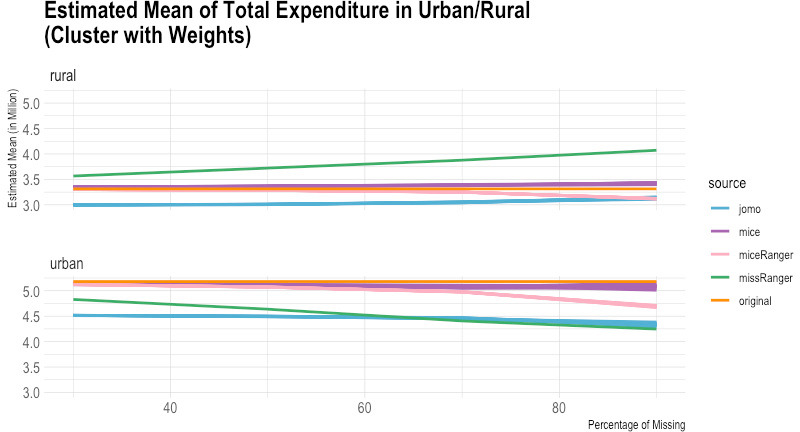
Figure 2.
Comparison of imputed and original total expenditure by urban/rural (standard error). Source: Author’s preparation.
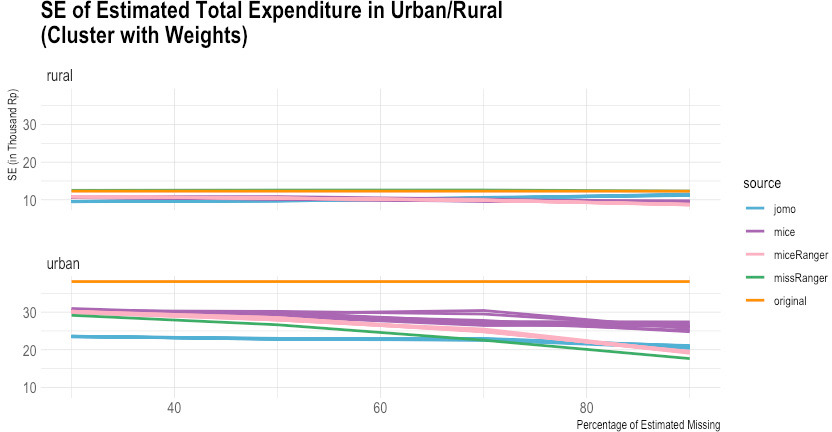
Figure 3.
Comparison of imputed and original total expenditure by province (estimated mean). Source: Author’s preparation.
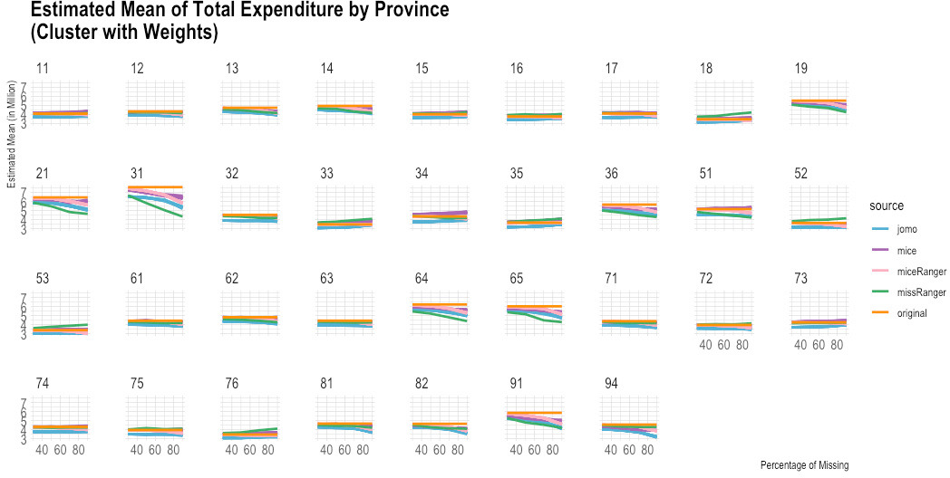
Figure 4.
Comparison of imputed and original total expenditure by province (standard error). Source: Author’s preparation.
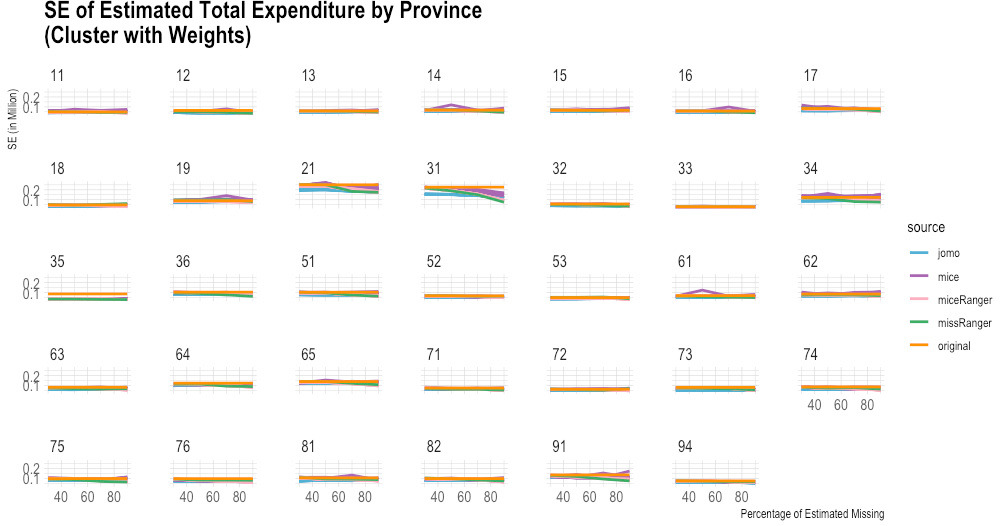
Figure 5.
Comparison of imputed and original total expenditure by household size (estimated mean). Source: Author’s preparation.
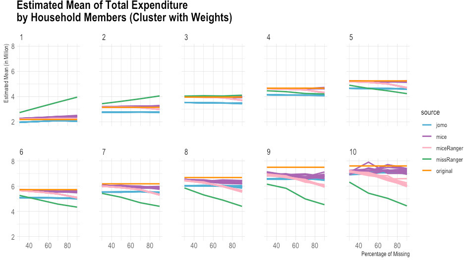
Figure 6.
Comparison of imputed and original total expenditure by household size (standard error). Source: Author’s preparation.
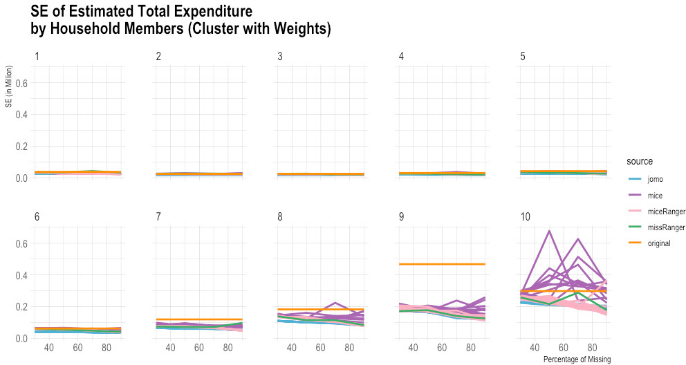
Figure 7.
Comparison of imputed and original total expenditure by employment status (estimated mean). Source: Author’s preparation.
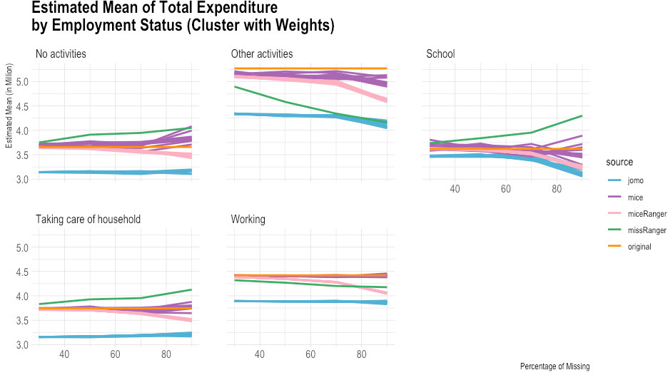
Figure 8.
Comparison of imputed and original total expenditure by employment status (standard error). Source: Author’s preparation.
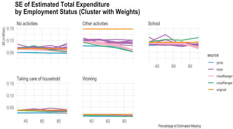
Figure 9.
Comparison of imputed and original total expenditure by education (estimated mean). Source: Author’s preparation.
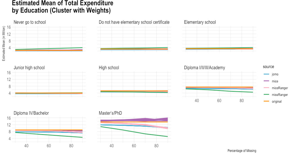
Figure 10.
Comparison of imputed and original total expenditure by education (standard error). Source: Author’s preparation.
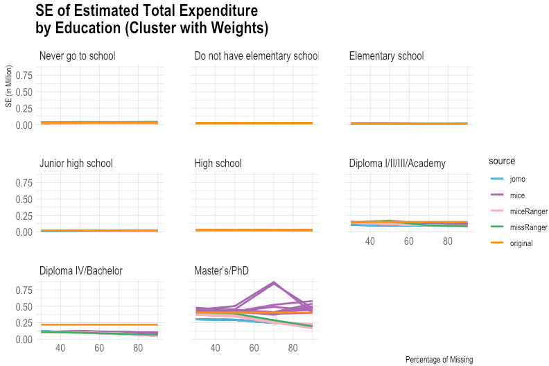
Table 3
Summary statistics of predictions from mice, jomo, and miceRanger: log (total expenditure)
| Percentage of missing | R packages | Min | Q1 | Med | Mean | Q3 | Max |
|---|---|---|---|---|---|---|---|
| 30% | mice | 13.54 | 14.66 | 14.95 | 15.00 | 15.27 | 18.59 |
| jomo | 13.50 | 14.66 | 14.95 | 15.00 | 15.28 | 18.64 | |
| miceRanger | 13.53 | 14.66 | 14.96 | 15.00 | 15.28 | 18.52 | |
| 50% | mice | 13.54 | 14.67 | 14.94 | 15.00 | 15.26 | 18.63 |
| jomo | 13.51 | 14.65 | 14.95 | 14.99 | 15.28 | 18.61 | |
| miceRanger | 13.56 | 14.67 | 14.96 | 15.00 | 15.28 | 18.44 | |
| 70% | mice | 13.59 | 14.67 | 14.94 | 15.00 | 15.26 | 18.69 |
| jomo | 13.41 | 14.64 | 14.94 | 14.98 | 15.27 | 18.47 | |
| miceRanger | 13.57 | 14.66 | 14.95 | 15.00 | 15.28 | 18.32 | |
| 90% | mice | 13.56 | 14.67 | 14.94 | 15.00 | 15.26 | 18.58 |
| jomo | 13.16 | 14.61 | 14.93 | 14.96 | 15.26 | 18.05 | |
| miceRanger | 13.61 | 14.63 | 14.92 | 14.97 | 15.25 | 18.08 |
Figure 11.
First and third imputed log(total expenditure) predictions. Source: Author’s preparation.
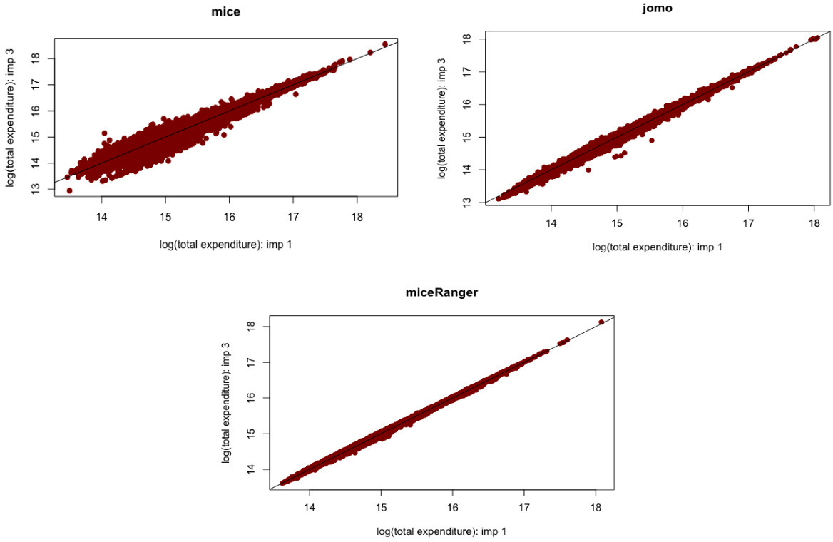
Table 4
Example of FMI: Model of log (total expenditure)
| Percentage of missing | ||||||||||||
|---|---|---|---|---|---|---|---|---|---|---|---|---|
| Variables | 30% | 50% | 70% | 90% | ||||||||
| jomo | mice | miceRanger | jomo | mice | miceRanger | jomo | mice | miceRanger | jomo | mice | miceRanger | |
| (Intercept) | 0.09 | 0.79 | 0.69 | 0.46 | 0.85 | 0.67 | 0.40 | 0.93 | 0.68 | 0.74 | 0.96 | 0.78 |
| (Employstat)2 | 0.14 | 0.72 | 0.40 | 0.23 | 0.85 | 0.41 | 0.47 | 0.93 | 0.40 | 0.78 | 0.98 | 0.55 |
| (Employstat)3 | 0.12 | 0.40 | 0.37 | 0.69 | 0.71 | 0.83 | 0.78 | 0.99 | 0.01 | |||
| (Edu)2 | 0.17 | 0.79 | 0.65 | 0.60 | 0.77 | 0.62 | 0.76 | 0.88 | 0.64 | 0.87 | 0.97 | 0.63 |
Note: 1. The negative values of FMI mean the package is underestimating the variability in the data. FMI was calculated using the following formula:
2. (Employstat)2 and (Employstat)3 are employment status variable for category 2 and 3. (Edu)2 is education variable for category 2. The default is category 1.
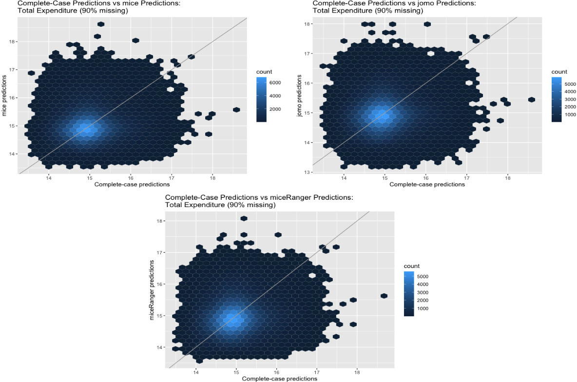
Figure 12.
Complete-case, mice, jomo, and miceRanger predictions. Source: Author’s preparation
In contrast to missRanger, jomo seems to work in capturing the variability in the data, but it has high bias because it tends to underestimate the original value. The results of jomo show the multilevel model approach cannot guarantee it will achieve a successful result of imputations, even though the data used is also in the form of multilevel. In addition to that, jomo is indeed very slow. It took 12 days on the server to run entirely until the Horvitz-Thompson estimator was calculated.
Although miceRanger was expected to combine the accuracy of mice and the speed of ranger, miceRanger could not achieved those two things in reality. The empirical evidence shows that miceRanger was far too slow compared to missRanger in which missRanger took only a few seconds, while miceRanger took around two days. Sometimes the accuracy of miceRanger was relatively good and stable if we look at the comparison of its imputed values with original data in terms of the estimated mean and standard error, crossed by some variables. However, the results are worse as seen by the higher the percentage of missing values.
The most accurate results were obtained from the mice package. The results of mice are reasonable, but it has a high variance, and some of the multiple imputations results could not achieve good accuracy in some categories. Nevertheless, mice can capture the variability in the data quite well in general. The first imputation results of mice seem reasonably similar to the original data, including most categories based on the break-down from the Horvitz-Thompson estimator. Those results give hope that running data using a computer can help in reducing respondent burden, time, and cost in data collection.
Data collection is not an easy task to do, in particular for a big archipelago country with complex conditions of social, culture, economics, environment (remote areas), educational background of its society, and disasters that can happen at any time (including disasters resulted from human behaviours, for example, caused by conflicts between two ethnicities). In fact, the interview to collect expenditure data may take at least two or three hours with the possibility of recall bias and measurement errors. Another finding from this study is that missing values from a census block can happen in reality, so the results obtained by using cluster sampling generated artificial missing values are important. In addition, the uncertainty of mice, jomo, and miceRanger is confirmed after combining the multiply-imputed data sets.
An important lesson from this study is that a greater understanding of the technique’s risks and weaknesses is needed before implementing a method for the imputation of census or survey data. An ideal condition according to MAR is that the spread of residuals for observed and imputed data should be similar (but not identical) because their distributions should overlap [17], mice and missRanger seem to achieve that. Nevertheless, handling such a vast data set needs a substantial computational effort, exceptionally to construct a model for the imputation of deliberately missing data from sub-sampling. A limited time in conducting this study is also a constraint in dealing with a very large data set, despite using a large memory computer.
2.2Combining multiply-imputed data sets
A total of ten data sets have resulted from each of mice, jomo, and missRanger in each scenario of different proportions of missingness. Multiply-imputed data sets were combined using mitools package to incorporate Rubin’s rule on multiple imputations. Summary statistics of predictions from the combined data sets are displayed in Table 3. According to the summary statistics, the prediction of log(total expenditure) yielded satisfactory results, except for the minimum and maximum values, which cannot be predicted accurately across a different proportion of missing values.
In order to look at the relationship between imputed values resulting from the same package, the relationship between predicted values from the first and third imputed data sets was presented. Figure 11 illustrates the relationship between predicted values produced based on mice, jomo, and miceRanger in the case of log(total expenditure) predictions. Overall, all predicted values based on the three packages are spread out close to the diagonal line, which means that the differences of the two imputed data sets are due to the fitted model or the trained model in miceRanger. The plot of predicted values from mice shows that mice has the most significant variability among the three packages. This evidence is in accordance with the Horvitz-Thompson estimator. In contrast, miceRanger’s predictions have the most negligible variability.
Figure 12 shows the comparison between complete-case and the three packages predictions for total expenditure (here log was used). The three plots are very similar; some of the prediction points are pretty far from the diagonal line.
3.Conclusions
Overall, it is possible to subsample expenditure data and impute for the deliberately missing data. The positives of sub-sampling are that we can gain efficiency in time and cost of data collection and reduce measurement issues and respondent burden. A week of running data using a computer is much cheaper and faster than data collection.
Furthermore, the comparison of four R packages in the case of Susenas data shows that reasonable results of imputations can be obtained from the mice package, but it still has weaknesses. Meanwhile, missRanger is not working in this study because it cannot capture the variability in the data. Although jomo is based on a multilevel model which is suitable to the Susenas data, the Horvitz-Thompson estimator shows that jomo has moderately high bias. In addition, miceRanger is very slow for a machine learning-based imputation method, and it cannot work when the percentage of missing is 90%.
In addition, more research is needed to explore more suitable methods that can be used to impute the expenditure data in the Susenas survey. The possibility is that we need to try to impute each province separately since each province has different characteristics or according to regencies with similar characteristics. Moreover, potential other methods that can be tried are neural network and XGBoost. Indeed, this study dealt with computational constraints because of using a very large data set, so there was a substantial computational effort in handling the data.
Acknowledgments
This paper is a part of my MSc dissertation (Department of Statistics, The University of Auckland). My supervisor was Prof. Thomas Lumley, BSc (Hons), MSc, PhD, FRSNZ. I studied at The University of Auckland as an employee of BPS-Statistics Indonesia, my study was funded by The New Zealand Ministry of Foreign Affairs and Trade.
References
[1] | Pistaferri L. Household consumption: research questions, measurement issues, and data collection strategies. Journal of Economics and Social Measurement. (2015) ; 40: (1-4): 123-149. |
[2] | Ritonga H. The impact of household characteristics on household consumption behavior: a demand system analysis on the consumption behavior of urban households in the province of Central Java, Indonesia. PhD thesis, Iowa State University. (1994) . |
[3] | Ahmad Z, Fatima A. Prediction of household expenditure on the basis of household characteristics. Proc ICCS-11. (2011) ; 21: : 351-367. doi: 10.13140/2.1.2507.5206. |
[4] | Azadeh A, Davarzani S, Arjmand A, Khakestani M. Improved prediction of household expenditure by living standard measures via a unique neural network: the case of Iran. International Journal of Productivity and Quality Management (IJPQM). (2016) ; 17: (2): 142. |
[5] | Dias JG, Oliveira ITd. Exploring unobserved household living conditions in multilevel choice modeling: an application to contraceptive adoption by Indian women. PLoS One. (2018) ; 13: (1). doi: 10.1371/journal.pone.0191784. |
[6] | Gao C, Fei CJ, McCarl BA, Leatham DJ. Identifying vulnerable households using machine learning. Sustainability 2020. (2020) ; 12: (15): 6002. doi: 10.3390/su12156002. |
[7] | Langkamp DL, Lehman A, Lemeshow S. Techniques for handling missing data in secondary analyses of large surveys. Acad Pediatr. (2010) ; 10: (3): 205-210. doi: 10.1016/j.acap.2010.. |
[8] | Schmitt P, Mandel J, Guedj M. A comparison of six methods for missing data imputation. J Biomed Biostat. (2015) ; 6: (1): 1-6. doi: 10.4172/2155-6180.1000224. |
[9] | Huque MH, Carlin JB, Simpson JA, et al. A comparison of multiple imputation methods for missing data in longitudinal studies. BMC Med Res Methodol. (2018) ; 18: (1): 168. doi: 10.1186/s12874-018-0615-6. |
[10] | Dumpert F. Machine learning for imputation. Federal Statistical Office of Germany (Destatis); (2020) . |
[11] | Little RJA, Rubin DB. Statistical analysis with missing data. 3rd ed. John Wiley & Sons, Inc. (2020) . |
[12] | Mayer M. missRanger: Fast imputation of missing values. R package version 2.1.0. (2019) . |
[13] | Wright MN, Ziegler A. ranger: A fast implementation of random forests for high dimensional data in C++ and R. Journal of Statistical Software. (2017) ; 77: (1): 1-17. doi: 10.18637. |
[14] | Wilson S. miceRanger: Multiple imputation by chained equations with random forests. R package version 1.4.0. (2021) . |
[15] | Quartagno M, Grund S, Carpenter J. jomo: A flexible package for two-level joint modelling multiple imputation. R Journal. (2019) ; 11: (2): 205-228. doi: 10.32614/RJ-2019-028. |
[16] | Stekhoven DJ, Bühlmann P. MissForest – non-parametric missing value imputation for mixed-type data. Bioinformatics. (2012) ; 28: (1): 112-118. doi: 10.1093/bioinformatics/btr597. |
[17] | van Buuren S, Groothuis-Oudshoorn K. mice: Multivariate imputation by chained equations in R. Journal of Statistical Software. (2011) ; 45: (3): 1-67. doi: 10.18637/jss.v045.i03. |
[18] | van Buuren S. Flexible Imputation of missing data. 2nd ed. Chapman and Hall/CRC; (2018) . |
[19] | Carpenter JR, Kenward MG. Multiple imputation and its application. 1st ed. London: John Wiley & Sons, Ltd.; (2013) . |
[20] | Lumley T. mitools: Tools for multiple imputation of missing data. R package version 2.4. (2019) . |
[21] | Lumley T. survey: Analysis of complex survey samples. R package version 4.0. (2020) . |


