
Integrating surveys with geospatial data through small area estimation to disaggregate SDG indicators: A practical application on SDG Indicator 2.3.1
Abstract
With the adoption of the 2030 Agenda for Sustainable Development, the production of high quality disaggregated estimates of Sustainable Development Goal (SDG) indicators has taken greater significance. In this context, sample surveys are characterized by samples that are either not large enough to guarantee reliable direct estimates for all relevant sub-populations, or that do not cover all possible disaggregation domains. To address these issues, indirect estimation approaches such as small area estimation (SAE) techniques can be adopted.
The literature on the use of SAE in official statistics is broad and in continuous progress, yet the number of case studies on SAE methods applied to SDG indicators can still be expanded. After a brief review of the main SAE approaches available along with their principal fields of application, the present paper aims contributing to fill this gap by presenting a case study on SAE to produce disaggregated estimates of SDG Indicator 2.3.1, measuring average labour productivity of small-scale food producers. The discussed empirical exercise is based on a Fay-Herriot area-level SAE model, integrating survey data with area-level auxiliary information retrieved from multiple trustworthy geospatial information systems. Area-level SAE models have the advantage of being easy to implement and do not require accessing survey microdata and unit-level auxiliary information. These characteristics, jointly with the great potentials offered by modern geospatial information systems, offer the possibility of producing good quality disaggregated estimates of SDG indicators at high frequency and granular disaggregation level.
1.Introduction
In an era characterized by the proliferation of new data sources and an unprecedented data revolution, the 2030 Agenda for Sustainable Development and the overall goal of leaving no-one behind (LNOB) have generated a tremendous increase in the demand of disaggregated data and statistics. In particular, in order to operationalize the overarching requirement of data disaggregation in the development of the Global SDG Indicator framework, the United Nations Statistical Commission postulated that “SDG Indicators should be disaggregated, where relevant, by income, sex, age, race, ethnicity, migratory status, disability and geographic location, or other characteristics, in accordance with the Fundamental Principles of Official Statistics”.
In this framework, traditional sample surveys implemented by National Statistical Offices (NSOs) can provide important information on the social, economic and environmental dimensions of target populations, representing the essential data source to produce the official estimates of about the 30% of Sustainable Development Goal (SDG) Indicators.11 However, these data sources alone are not enough to realize the ambitious goal of monitoring SDG Indicators by all relevant disaggregation dimensions and geographical areas. Indeed, despite collecting detailed information at relatively high frequency, most sample surveys are characterized by sample sizes that are either not large enough to guarantee reliable direct estimates for all sub-populations or that do not cover all possible disaggregation domains [1].
Issues of this kind can be addressed at different stages of the statistical production process. They can be tackled at the design stage, by adopting sampling strategies guaranteeing an observed set of sampling units for every disaggregation domain. Although potentially optimal, this approach normally results in an exponential increase of the sampling size and survey costs and complexity [2]. Furthermore, it is important to realize that, in practice, the anticipation of all possible future uses of survey data is virtually impossible, as “the client will always require more than is specified at the design stage” [3]. Alternatively, data disaggregation can be addressed at the data analysis stage, by adopting indirect estimation approaches borrowing strength from related disaggregation domains and/or time periods, thus resulting in an increase of the effective sample size [4]. Small area estimation (SAE) methods are among the possible indirect estimation approaches that can be adopted to deal with data disaggregation at the analysis stage. SAE techniques allow combining survey data with auxiliary information coming from additional data sources that are not affected by sampling error. Traditionally, SAE have relied on the integration of survey microdata with information from population and agricultural censuses or administrative records through explicit models linking the variable of interest to a set of auxiliary variables. However, with more and more data made available to National Statistical Systems (NSSs) from multiple innovative data sources, relying exclusively on auxiliary variables from traditional statistical sources for the production of small area estimates of SDG indicators is not considered as an efficient solution. In this respect, the 2030 Agenda explicitly stresses the need for new and enhanced data integration strategies, including the exploitation of the potential contribution to be made by geospatial information systems and other big data sources.
Within this framework, the present paper makes the case for the adoption of SAE and other indirect estimation methods to produce granular disaggregated estimates of SDG indicators, by integrating survey microdata with auxiliary information retrieved from “innovative” data sources, such as earth observation data. Indeed, relying on suitably implemented indirect estimation techniques such as SAE allows obtaining reliable disaggregated estimates of SDG indicators while managing survey costs and complexity. In particular, the integration of survey microdata with data from non-traditional sources offers the potential of producing timelier and more disaggregated statistics at higher frequencies than what allowed by traditional data sources alone. The paper is structured as follows. Distinguishing between area-level and unit-level SAE models, Section 2 presents a brief overview of these two approaches along with their relevant notation, context of usability, and potential source of auxiliary data. This section also discusses the main strengths and elements of cautions related to the use of geospatial auxiliary variables. Then, Section 3 presents some of the main fields of SAE application in official statistics, highlighting the few initiatives and examples of SAE for data disaggregation of official SDG indicators. To fill the gap of SDG relevant studies, Section 4 presents a practical case study on SDG indicator 2.3.1, measuring the average volume of production per labour unit of small-scale food producers, based on the Fay-Herriot (FH) [5] area-level model and combining the official integrated household survey of Mali with auxiliary variables retrieved from multiple geospatial information systems. The results of the case study highlight that, implementing the considered SAE approach, estimates precision is improved and predictions for out-of-sample domains can be produced. Finally, the main conclusions and ways forward are presented in Section 5.
2.Integrating survey data with additional data sources through small area estimation
Sample surveys, which are regarded as cost-effective means to collect detailed information at relatively high frequency over time, have a long history in the field of official statistics, and can be used to produce reliable estimates of parameters referred to total populations or to broad disaggregation domains. In this context, direct domain estimates of target parameters are statistics based solely on domain-specific sample data. Direct estimators are also known as design-based estimators, since they make use of sampling weights to produce inference on the target population [6]. One of the main requirements to achieve reliable disaggregated estimates by direct estimators is the presence of a sufficient domain sample size to yield adequate precision, or, in other words, a small estimated variance. When this circumstance is not verified, we are in the presence of so-called small-areas, i.e. disaggregation domains for which too little or no sampling observations are available [4]. It should be noted that, in practical statistical applications, it is quite rare to have an overall sampling size that is large enough to guarantee a sufficient number of observations for every possible disaggregation domain. Therefore, the use of indirect estimation techniques that “borrow strength” from auxiliary information on the population of interest [7] is often necessary. The range of possible approaches to produce indirect estimators is vast and goes from the implementation of design-based model-assisted approaches, such as the generalized regression estimator ([8, 9]) or the projection estimator ([10, 11]), to model-based approaches such as SAE ([4, 5, 12]). Contrarily to direct and model-assisted approaches, SAE model-based methods rely on explicit models and, consequently, the properties of resulting estimators are assessed under the adopted model assumptions. In particular, traditional SAE models are mixed models with area-specific random effects accounting for the variability between different areas not explained by auxiliary variables [4].
Although different in their specification, all SAE approaches share the same notation framework that is here introduced for the clarity of following sections. Let us consider a finite population
Direct HT estimators
Despite their increasing popularity, resorting to SAE should not be considered as the solution to any data disaggregation problem, and there are various considerations that NSOs should make before engaging in the production of indirect estimates. First of all, model-based approaches have stricter data requirements than direct estimation methods, with unit-level models being more data intensive than area-level ones. In this respect, the access to microdata on individual units may be limited by confidentiality concerns that need to be taken into account. Being based on models, after implementing SAE approaches, the underlying assumptions need to be carefully validated through adequate diagnostic techniques [27]. In addition, the bias of small area estimates needs to be measured to assess estimates reliability. This is generally done by means of the mean square error (MSE), which provides a combined indicator of estimates precision (variance) and accuracy (bias).
2.1Area-level SAE models
The FH model [5], which is by far the most popular area-level SAE approach, is often used for the production of small area estimates in official statistics and research thanks to its intuitive application and interpretation. This approach combines a sampling model, assuming that the unknown parameter
(1)
where
The unknown parameters of Eq. (1) to be estimated are the fixed-effects parameters
One of the FH fundamental assumptions of known variances
2.2Unit-level SAE models
Contrarily to area-level approaches, unit-level SAE models require the availability of unit-level microdata for both the variable of interest
(2)
where
The model in Eq. (2.2) contains independent and identically distributed (iid) domain-specific random effects
Under the EBLUP approach, the SAE estimator can be formalized as a linear combination of the survey regression estimator and a regression-synthetic component:
Where
measures the amount of unexplained between-area variability to the total variability, and gives more importance to the survey regression component of the estimator with increasing domain sample size
Similarly to what seen for area-level models, various extensions of the basic unit-level approach are available in the literature. In particular, while the model in Eq. (2.2) only supports the estimation of means and totals, approaches relying on nested error linear regression models allow the estimation of non-linear indicators ([24, 25]). These extensions are particularly relevant in the context of the SDG monitoring framework, where many of the indicators are expressed as ratios and proportions. Additional extensions allow to include sampling weights in the estimation process [26], address the presence of heteroscedasticity in the error term [20], and produce estimates which are robust to influential outliers [21].
2.3Some practical considerations on SAE implementation with different types of auxiliary data
An important prerequisite for the construction of SAE models with satisfactory predictive power is the availability of good quality auxiliary variables that can properly explain the phenomenon under study. Traditionally, this additional information for SAE implementation has been extracted from population and agricultural censuses or administrative records. Census data have the advantage of providing a complete coverage of the target population and can offer valid socio-economic predictors of the variable of interest. However, the low frequency at which censuses are normally implemented limits their use for the production of disaggregated statistics on an annual basis. On the other hand, administrative records, which are often generated as side product of government operations, do not suffer from this drawback. However, this second type of data are not produced with the primary purpose of computing official statistics, and, as a consequence, their accuracy, coverage, content, and characteristics need to be carefully assessed before them being used for statistical purposes [28]. The merits and demerits of administrative data in the production of official statistics are extensively discussed in [29]. Some examples of applications of SAE based on administrative records are given in [4, 28, 30].
The huge amount of digital and geospatial information produced by a wide range of tools and technologies nowadays offers good alternative sources of auxiliary variables for SAE production. These rich large-scale datasets, often referred to as big data, generally cover a vast portion of the population within a territory, often reaching nationwide coverage. Potential sources of big data are geospatial information systems, social networks, and records generated by human transactions and interactions. These “new” or “alternative” data sources can complement traditional surveys and censuses to reduce the time and resources needed for data production, hence contributing to fill the SDG data gap. For example, latest available geospatial technologies can not only provide the auxiliary information to implement SAE or other indirect estimation approaches, but can also help improving the construction of master sampling frames and producing direct estimates of selected SDG indicators (e.g. indicator 15.1.1 on the percentage of forest area on total area, and indicator 15.4.2 measuring changes in the mountain green cover).
Examples of studies relying on the use of big data and geospatial information for the implementation of SAE techniques are presented in [31, 32, 33, 34]. In particular, in [31], the authors discuss the challenges opened by the extension of SAE covariates to include variables generated by big data sources and provides some solutions to address them. Specifically, besides requiring the availability of advanced statistical and IT know-how, the quality of data from these “new” data sources is often uncertain and rarely documented in comprehensive metadata files. In this respect, attention should be paid to the fact that basic SAE approaches are implemented under the assumption that auxiliary variables are measured without error, or, in other words, that they are available for all areas and they come from archives covering the entire population of interest. However, data coming from big data sources are often affected by measurement errors and bias. Various authors (e.g. [22, 35]) have addressed this issue by developing SAE approaches accounting for the presence of measurement errors in the covariates.
When using big data retrieved by earth observation systems, particular attention should be paid at the definition and computation of the covariates included in the model. Indeed, geospatial variables are usually available at the levels of the cells of regular grids of different resolutions, and need to be rescaled in order to be attributed either to individual sampling units (for unit-level approaches) or to the irregular polygons representing the estimation domains (for area-level approaches). Hence, when implementing area-level models such as the one summarized by expression (1), the value
3.Use of small area estimation approaches for data disaggregation of SDG indicators
The empirical literature on SAE is very broad, with applications in many different fields of official statistics such as income and poverty, labour, health and agriculture. However, despite the great emphasis placed on data disaggregation in the context of the SDG monitoring framework and its overarching LNOB pledge,33 the number of examples of SAE techniques applied to official SDG indicators is still limited.
Being poverty mapping among the main applications of SAE, several case studies and references are available for the disaggregation of indicators related to Goal 1 on ending poverty. In particular, SAE techniques have been implemented to produce official sub-national estimates of SDG indicators 1.1.1 and 1.2.144 in countries such as Albania, Bolivia, Bulgaria, Cambodia, Chile, Ecuador, Indonesia, Mexico, Morocco and Sri Lanka ([23, 36]). Other applications relevant to income and poverty analysis, yet without a direct link with SDG indicators, can be found, for example, in Tanzania [37] and the United States [38].
Concerning Goal 2, aiming at ending hunger, achieving food security, improving nutrition and promoting sustainable agriculture, applications of SAE relevant to food security and malnutrition were found in Nepal [39], Ethiopia [40], and the United States [41]. However, the only application of indirect estimation techniques targeting specifically an indicator under Goal 2 was developed by the Food and Agriculture Organization of the United Nations (FAO) for indicator 2.1.2 on the prevalence of moderate and severe food insecurity in the population based on the food insecurity experience scale ([1, 11]). Concerning the agricultural component of Goal 2, evidence of empirical applications of SAE targeting SDG indicators under this goal were not found. Indeed, while SAE approaches have extensively been used to produce disaggregated estimates of crop yield and production measures (see [33, 34] for some examples), the use of indirect estimation approaches to produce disaggregated measures of agricultural labour productivity (indicator 2.3.1) or agricultural sustainability (2.4.1) are not a common practice.
Finally, a limited number of applications of SAE on indicators under Goal 4 [42], 5 [43], and 8 [44] were identified.
Table 1
Sampling size information for Mali’s Enquête Agricole de Conjoncture Intégreée aux Conditions de Vie de Ménages (EAC-I) 2017
| Region | Number of circle | Sample size by regio | Sample size of small-scale food producers by regio | Average num. of sampled small-scale food producers by circle |
|---|---|---|---|---|
| Kaye | 7 | 431 | 384 | 55 |
| Koulikor | 7 | 381 | 282 | 40 |
| Sikass | 7 | 368 | 206 | 29 |
| Sego | 7 | 436 | 295 | 42 |
| Mopt | 8 | 326 | 221 | 28 |
| Tombouctou | 5 | 137 | 126 | 63 |
| Ga | 3 | 110 | 101 | 34 |
| Kida | 4 (out of sample | – | – | – |
| Menaka | 4 (out of sample | – | – | – |
| 1 (Bamako) | 22 | 22 | 22 |
4.Empirical application of SAE on SDG Indicator 2.3.1 with the use of geospatial auxiliary variables
Target 2.3 of the 2030 Agenda for Sustainable Development aims to double the agricultural productivity and incomes of small-scale food producers by the end of the monitoring period. Progress towards the achievement of this target is monitored by two official SDG indicators, namely indicator 2.3.1 – measuring the average value of agricultural production per labour unit55 – and indicator 2.3.2 – estimating the average income from agricultural production activities of small-scale food producers. Indicator 2.3.1, which is the object of the presented case study, provides a measure of average partial factor productivity of agricultural holdings in a given year, and is currently disaggregated by the sex of the holding’s head and the size of the farm (small versus non-small). In particular, small-scale food producers are identified through an official definition developed by the FAO and endorsed by the Inter-Agency and Expert Group on SDG Indicators in September 2018 [45] in order to enhance international comparability. Although disaggregation at the subnational level is not among the mandatory disaggregation dimensions for reporting indicators under target 2.3, local estimates of indicators 2.3.1 and 2.3.2 may prove to be way more relevant than national aggregates for effective monitoring and decision making at the country level.
The typical data sources used to estimate SDG indicators on small-scale food producers are agricultural surveys, or household surveys integrated with modules on households’ agricultural activities. Being based on sample data, the production of reliable estimates of these two indicators at granular subnational level is usually not possible with standard design-based approaches, and –consequently – indirect estimation approaches need to be explored. As discussed in Section 3, the literature on small area income estimation is considerably wide, even if not necessarily targeting the estimation of incomes generated through agricultural production activities. Contrarily, the body of work on SAE approaches applied to indicators of labour productivity measures is still very little. In order to fill this gap, this section explores the application of a FH area-level model to produce small area estimates of SDG indicator 2.3.1 at the second administrative level (circles) of Mali, considering the integration of household survey data with area-level auxiliary information retrieved by multiple trustworthy geospatial information systems. Specifically, the presented SAE application is based on microdata from the Enquête Agricole de Conjoncture Intégrée aux Conditions de Vie de Ménages (EAC-I) 2017. The EAC-I is a multi-thematic cross-sectional household survey, implemented under the World Bank Living Standard Measurement Study (LSMS) programme, based on a nationally representative sample of about 8,390 households and with a specific focus on agriculture. In 2017, the sample units were divided into two groups, one of 3,813 households that received the full questionnaire, and one with remaining households that received a light version of the same questionnaire. For the purpose of this application, only the group of households that completed the full questionnaire could been considered, since this included the necessary variables to identify small-scale food producers and compute the targeted indicator. Considering that indicator 2.3.1 has a disaggregation dimension already embedded in its definition, i.e. the size of the farm, the sample that could be used to produce small area estimates for small scale food producers included only 1,637 households. Table 1 provides a summary of the sample size by region and circle, and the number of out-of-sample circles. In particular, the entire region of Kidal was left outside of the sample due to security reasons. In addition, the new region of Menaka had not been officially announced yet at the time of the survey and, for this reason, was not included in the sample.
Table 1 provides information on the sampling size by region and circles.
4.1Parameter of interest, selection of SAE approach, and considered geospatial auxiliary variables
Going back to notation introduced in Section 2, the average volume of production per labour unit to be estimated in each small area can be formalized as
Table 2
Spatio-temporal resolution and sources of geospatial area-level covariates
| Variable name | Spatial resolution | Temporal resolution | Source |
|---|---|---|---|
| Vol. fraction of coarse fragments | 1 | Static | ISRIC: World Soil Information |
| Nitrogen | 1 | Static | |
| Sand | 1 | Static | |
| Silt | 1 | Static | |
| Clay | 1 | Static | |
| Soil organic carbon | 1 | Static | |
| Minimum temperature | 4.5 | Monthly | WorldCilm: Historical monthly weather data |
| Maximum temperature | 4.5 | Monthly | |
| Precipitation | 4.5 | Monthly | |
| Direct normal irradiation (Long-term yearly average) | 0.3 | 1994-2018 | Solargis |
| Diffuse horizontal irradiation (Long-term yearly average) | 0.3 | 1994–2018 | |
| Air temperature (Long-term yearly average) | 1 | 1999–2018 | |
| Vegetation indexes | 5.5 | Monthly | NASA EarthData |
| Elevation | 1 | Static | CGIAR CSI |
| Cropland | 1 | Annual | Zenodo |
| Bare ground | 1 | Annual | |
| Built-up | 1 | Annual | |
| Harvested area (major crops) | 1 | Annual | MAPSPAM |
| Production (major crops) | 1 | Annual |
The accuracy of direct estimates, measured in terms of the estimated coefficient of variation (CV), was assessed against the same accuracy measure produced for EBLUP small area estimates obtained with the FH model in expression (1). This approach was selected in place of a unit-level method in order to produce a case study on SAE based on a model of simple implementation, only requiring access to area-level direct estimates and auxiliary information. In addition, as seen in Section 2.1, the EBLUP area-level estimator obtained from the model presented in expression (1) can be formulated as a linear combination of area-level direct and synthetic estimates, giving more weight to the former with increasing sampling size. Hence, using the FH SAE model can intuitively be seen as a way of improving direct estimates through a synthetic component based on external information. On the other hand, unit-level estimators, such as the one introduced in expression 2.2, do not take into account direct estimates and – as a consequence – the sampling design.
As area-level auxiliary variables for the implementation of the small area estimation model, various geospatial covariates were considered among the vast amount of publicly available candidates according to their potential capability of being good predictors for the average labour productivity in agriculture. In particular, covariates included in the first stage of selection were providing information on the following domains:
• Soil characteristics: volume fraction of coarse fragments (
• Weather and climate: minimum and maximum temperature, precipitation quantity, direct normal irradiation, diffuse horizontal irradiation, air temperature, vegetation indexes.
• Land cover: elevation, cover fraction of cropland, bare ground and extent of built up areas.
• Harvested area and production of major crops (cotton, rice, sorghum, and wheat).
Table 2 presents the spatial and temporal resolution of each auxiliary variable along with the related source.
Table 3
Results of step-wise regression
| Variable name | Unit of measure | lmg (%) |
|---|---|---|
| Production of cotton | (Metric ton) | 24.0 |
| Direct normal irradiation | (kWh/m2) | 16.1 |
| Production of wheat | (Metric ton) | 14.6 |
| Production of rice | (Metric ton) | 11.7 |
| Production of sorghum | (Metric ton) | 11.4 |
| Vol. fraction of coarse fragments | (%) | 9.8 |
| Soil organic carbon | (g kg-1) | 8.7 |
| Harvested area of rice | (hectare) | 3.7 |
Values of considered geospatial predictor were initially available at the level of the cells of regular grids of different resolutions (spanning from 1
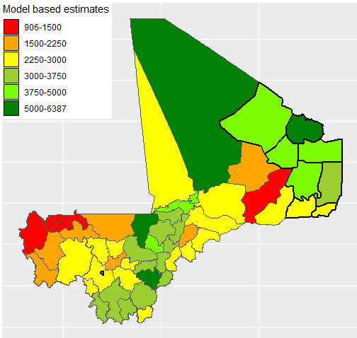
Figure 1.
Small area estimates of indicator 2.3.1 in Mali disaggregated by circle (second administrative division).
The initial set of potential predictors was then reduced adopting a stepwise regression, which was implemented using the area-level direct estimates of indicator 2.3.1 as dependent variable and the geospatial covariates as regressors.77 As result of the step-wise regression, only 8 auxiliary variables were retained (see Table 3) according to the Lindeman Merenda and Gold (LMG) factor, which represents a measure of the relative contribution of each predictor to the overall R square of the model. It is interesting to notice that most of the covariates considered as important by the selection approach provide information on either the quantity produced or the area harvested of Mali’s major crops. Other variables retained by the stepwise procedure measure the average direct normal irradiation, the average volume fraction of coarse fragments, and the average quantity of organic carbon in the soil.
4.2Smoothing variance of direct estimates
As seen in Section 2, among the necessary inputs to produce EBLUP small area estimates there are the estimated variances of direct estimates
Figure 2.
Boxplot of direct (left) and small area (right) estimates.
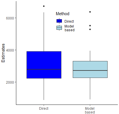
Figure 3.
Accuracy of direct and small area estimates and assessment of their linear relationship.
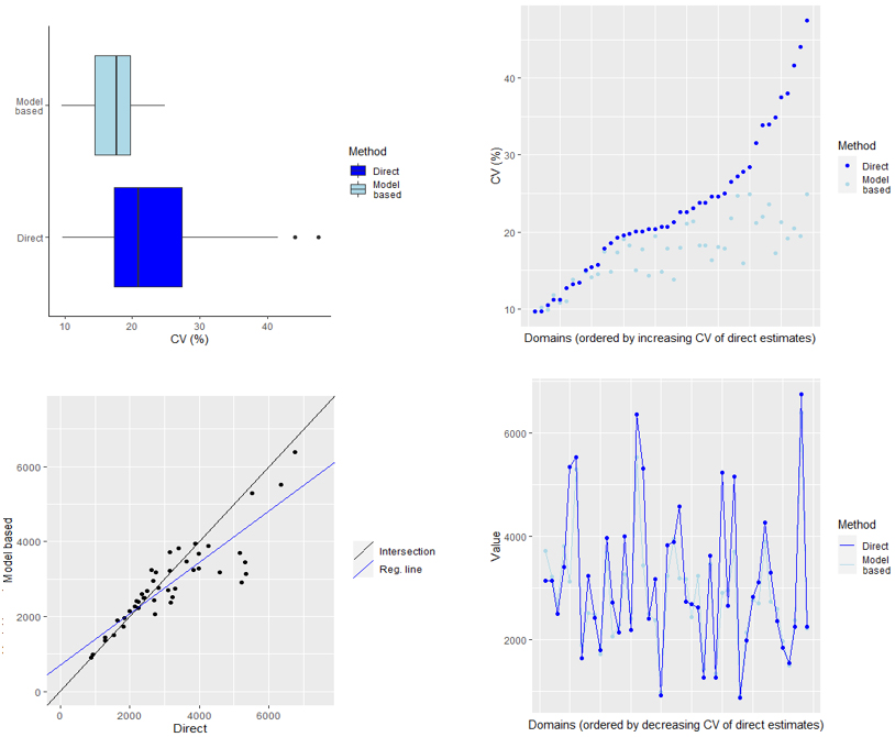
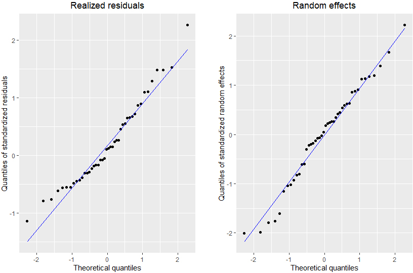
Figure 4.
Residuals and random effects of SAE model.
4.3Results assessment and model validation
The map presented in Fig. 1 displays the obtained small area estimate for each circle of Mali (including out of sample circles, which are identified with ticker borders). Values of indicator 2.3.1 range from 906 West African CFA Franc per labour unit in the circle of Kayes to 6387 in Niono, with the highest values of agricultural labour productivity predicted in northern and central circles. The two boxplots presented in Fig. 2 provide a first evidence of the fact that the obtained small area estimates (boxplot on the right) have a much lower variability compared to direct ones (boxplot on the left).
The four graphs presented in Fig. 3 allow comparing the accuracy of direct and indirect estimates in terms of their CVs, and assessing the presence or absence of linear relationship between the two groups of statistics. In particular, the two boxplots in the top-left quadrant of Fig. 3 display the distribution of CVs of direct and model-based estimates and highlights the higher accuracy of small area estimates compared to their design-based counterpart. Indeed, small area estimates’ CVs falls below the 20% in 3/4 of the cases, while the same threshold is surpassed by more than the 50% of direct estimates. Similar evidence is provided by the plot on the top-right corner, where direct and indirect estimates are ordered by increasing values of their CV. This provides a visual indication of the fact that the CV of small area estimates falls always below the same variability measure referred to direct estimates, except in the very few cases where the domain direct estimates were already showing a high accuracy (i.e. CV below 15%).
The graph on the bottom-left corner allows assessing the linear relationship between direct and indirect estimates. Generally speaking, especially in correspondence of domains with sufficient sampling size, direct and indirect estimates are expected to be correlated, meaning the two approaches should produce similar estimation results. In the considered case, the graphs illustrate a fairly strong linear relationships between estimates produced with the two approaches, with correlation equal to 0.88.
After assessing estimates accuracy, an important component of SAE implementation is the validation of fundamental assumptions underlying the model, i.e. the normality of residuals and random effects. To that purpose, Fig. 4 presents the QQ plots of both the error term and the random effects, which does not provide any significant proof of deviation from the normality assumption. This was also confirmed by the Shapiro-Wilk test, which resulted in
5.Conclusions and way forward
Monitoring the implementation of the 2030 Agenda for Sustainable Development and its overarching pledge to leave no one behind calls for more disaggregated data and SDG indicators than what available in most countries. In this context, sample surveys are the preferred data source for about the 30% of indicators in the SDG monitoring framework and can offer valuable information to measure the social, economic and environmental dimensions of sustainable development. However, traditional households and agricultural surveys are usually characterized by sampling sizes that are either too small to produce precise estimates, or that do not cover all disaggregation domains of interest. Hence, indirect estimation approaches such as SAE techniques can represent a valuable tool for NSOs and international organization to produce timely and granular disaggregated estimates of SDG indicators, allowing to contain the cost and complexity otherwise generated by the increase of sampling sizes. In particular, with the proliferation of new data sources such as geospatial and big data information systems, SAE models can be implemented by combining survey data with a vast amount of auxiliary information available at no or limited cost and at high frequency. In this respect, the body of literature and the number of case studies on SAE techniques applied to SDG Indicators can still be expanded. After a brief review of the main SAE approaches available along with their principal domains of application, this paper presents a case study based on the Fay-Herriot area-level SAE model to produce subnational estimates of SDG Indicator 2.3.1 on the average volume of production per labour unit obtained by small-scale food producers. This is done by integrating survey data with area-level auxiliary information retrieved from multiple geospatial information systems. The presented case study shows how the small area estimates of indicator 2.3.1 in Mali’s circles reach greater precision compared to direct estimates. In addition, adopting the considered indirect estimation approach, estimates for out of sample areas can also be produced.
The FH area-level model was selected in place of a unit-level method in order to provide a simple example of SAE based on an SDG indicator related to the agricultural sector development, only requiring access to area-level direct estimates and auxiliary information. In addition, using an indirect estimator – such as the area-level EBLUP – expressed as a linear combination of area-level direct and synthetic estimates, the SAE approach can intuitively be interpreted as a way of improving direct estimates through a synthetic component based on external information correlated with the phenomenon of interest. Future extensions of this study will compare the results obtained with the here considered area-level model with those produced by a unit-level approach. In this circumstance, both unit-level and sub-area (e.g. the enumeration area of the cell of a regular grid) level auxiliary variables will be considered as regressors.
Notes
1 This figure was presented in a mapping prepared by the Intersecretariat Working Group on Household Surveys and discussed at the 50
2 For the estimation of the domain total or mean and in order to implement basic unit-level SAE models, the selected auxiliary data source only needs to provide exact values of the domain means
3 Since its creation, the Inter-Agency and Expert Group on SDG Indicators (IAEG-SDGs), which was tasked with developing and implementing the SDG Global Indicator Framework, has included work on data disaggregation on its annual activities. In particular, the IAEG-SDGs formed a working group on data disaggregation and a task force on small area estimation for SDG indicators, with the purpose of developing standards and guidelines on data disaggregation and SAE for the SDGs.
4 SDG indicators 1.1.1 and 1.2.1 respectively measure the proportion of population living below the international and national poverty lines.
5 For the purpose of monitoring indicator 2.3.1, a labour unit is defined as one day of full time work.
6 All pre-processing data manipulations were performed with the R package “raster”.
7 An initial set of variables was eliminated due to their high correlation (above 0.9) with other covariates considered important, in order to avoid multicollinearity issues.
Acknowledgments
The authors are thankful to Stefano Falorsi, Senior Statistician and Chief of Unit at the Italian National Institute of Statistics (ISTAT), who provided relevant technical advice on models and software tools to improve the case study.
References
[1] | Falorsi PD, Donmez A, Khalil CA, Di Candia S, Gennari P. Alternative Methods for Disaggregating Sustainable Development Goal Indicators Using Survey Data. Statistical Journal of the IAOS. (2022) . doi: 10.3233/SJI-210901. |
[2] | Asian Development Bank. Introduction to Small Area Estimation Techniques. A Practical Guide for National Statistical Offices. Manila, Philippines; (2020) . |
[3] | Fuller WA. Environmental surveys over time. Journal of Agricultural, Biological and Environmental Statistics. (1999) ; 4: : 331–345. |
[4] | Rao JNK, Molina I. Small Area Estimation. Second Edition. Wiley. New York; (2015) . |
[5] | Fay RE, Herriot RA. Estimates of income for small places: An application of james-stein procedures to census data. Journal of the American Statistical Association. (1979) ; 74: (366): 269–277. |
[6] | FAO. Guidelines for data disaggregation of SDG indicators using survey data. Rome. Italy. (2021) . |
[7] | Giusti C, Masserini L, Pratesi M. Local comparisons of small area estimates of poverty: An application within the tuscany region in Italy. Soc Indic Res. (2017) ; 131: : 235–254. |
[8] | Cassel CM, Sarndal CE, Wretman JH. Some results on generalized difference estimation and generalized regression estimation for finite populations. Biometrika. (1976) ; 63: (3): 615–620. |
[9] | Särndal CE, Swensson B, Wretman J. Model Assisted Survey Sampling. Springer-Verlag; (1992) . |
[10] | Kim JK, Rao JNK. Combining data from two independent surveys: A model-assisted approach. Biometrika. (2012) ; 99: (1): 85–100. |
[11] | FAO. An indirect estimation approach for disaggregating SDG Indicators using survey data. A case study based on SDG Indicator 2.1.2. Rome, Italy. (2022) . |
[12] | Battese GE, Harter RM, Fuller WA. An error-components model for prediction of county crop areas using survey and satellite data. Journal of the American Statistical Association. (1988) ; 83: (401): 28–36. |
[13] | Cochran WG. Sampling Techniques. New York City, USA, John Wiley & Sons; (1977) . |
[14] | Wolter KM. Introduction to Variance Estimation. Second edition. New York. Springer-Verlag; (2007) . |
[15] | Harville DA. Comment. Statistical Science. (1991) ; 6: : 35–39. |
[16] | Morris CN. Parametric empirical bayes inference: Theory and applications. Journal of the American Statistical Association. (1983) b; 78: : 47–54. |
[17] | Browne WJ, Draper D. A comparison of bayesian and likelihood-based methods for fitting multilevel models. Bayesian Analysis. (2006) ; 1: : 473–514. |
[18] | Petrucci A, Salvati N. Small Area Estimation for spatial correlation in watershed erosion assessment. Journal of Agricultural, Biological and Environmental Statistics. (2006) ; 11: (2): 169–182. |
[19] | Marhuenda Y, Molina I, Morales D. Small area estimation with spatio-temporal Fay-Herriot models. Computational Statistics and Data Analysis. (2013) ; 58: : 308–325. |
[20] | Breidenbach J, Magnussen S, Rahlfa J, Astrupa R. Unit-level and area-level small area estimation under heteroscedasticity using digital aerial photogrammetry data. Remote Sensing of Environment. (2018) ; 212: : 199–211. |
[21] | Schoch T. Robust unit-level small area estimation: A fast algorithm for large dara sets. Austrian Journal of Statistics. (2012) ; 41: (4): 243–265. |
[22] | Ybarra LMR, Lohr SL. Small area estimation when auxiliary information is measured with error. Biometrika. (2012) ; 95: (4): 919–931. |
[23] | Bedi T, Coudouel A, Simler K. More Than a Pretty Picture: Using Poverty Maps to Design Better Policies and Interventions. Washington DC. World Bank. (2007) . |
[24] | Elbers C, Lanjouw J, Lanjouw P. Micro-level estimation of poverty and inequality. Econometrica. (2003) ; 71: : 355–364. |
[25] | Molina I, Rao JNK. Small area estimation of poverty indicators. The Canadian Journal of Statistics. (2010) ; 38: : 369–385. |
[26] | You Y, Rao JNK. A pseudo empirical best linear unbiased prediction approach to small area estimation using survey weights. The Canadian Journal of Statistics. (2002) ; 30: : 431–439. |
[27] | Eurostat. Guidelines on small area estimation for city statistics and other functional geographies. European Union. (2019) . |
[28] | Erciulescu AL, Franco C, Lahiri P. Use of administrative records in small area estimation. Administrative records for survey methodology. John Wiley & Sons, Inc.; (2021) ; 231–267. |
[29] | Brackstone GJ. Small Area Data: Policy Issues and Technical Challenges. In R. Platek, J.N.K. Rao, C.-E. Sarndall, and M.P. Singh (Eds.), Small Area Statistics. New York. John Wiley & Sons, Inc.; (1987) . pp. 3–20. |
[30] | Zhang LC, Giusti C. Small Area Methods and Administrative Data Integration. In: Analysis of Poverty Data by Small Area Estimation. John Wiley & Sons, Ltd; (2016) . |
[31] | Marchetti S, Giusti C, Pratesi M, Salvati N, Giovannotti F, Pedreschi D, Rinzivillo S, Pappalardo L, Gabrielli L. Small area model-based estimation using big data sources. Journal of Official Statistics. (2015) ; 31: (2): 263–281. |
[32] | Porter AT, Holan SH, Wikle CK, Cressie N. Spatial fay-herriot models for small area estimation with functional covariates. Spatial Statistics. (2014) ; 10: : 27–42. |
[33] | Ambrosio Flores L, Iglesias Martínez L. Land cover estimation in small areas using ground survey and remote sensing. Remote Sensing of Environment. (2000) ; 74: (2): 240–248. |
[34] | Singh R, Semwal DP, Rai A, Chhikara RS. Small area estimation of crop yield using remote sensing satellite data. International Journal of Remote Sensing. (2002) ; 23: (1). |
[35] | Arima S, Bell WR, Datta GS, Franco C, Liseo B. Multivariate Fay-Herriot Bayesian estimation of small area means under functional measurement error model. Journal of the Royal Statistical Sociery – Series A. (2018) ; 180: (4): 1191–1209. |
[36] | Casas-Cordero Valencia C, Encina J, Lahiri P. Poverty Mapping for chilean Comunas. In: Analysis of Poverty Data by Small Area Estimation. John Wiley & Sons, Ltd. |
[37] | Masaki T, Newhouse D, Silwal AR, Bedada A, Engstrom R. Small Area Estimation of non-monetary poverty with geospatial data. Policy Research Working Paper 9383. Poverty and Equity Global practice. The World Bank Group. (2020) . |
[38] | Bell WR, Basel WW, Maples JJ. An Overview of the US Census Bureau’s Small Area Income and Poverty Estimates Program. In: Analysis of Poverty Data by Small Area Estimation. John Wiley & Sons, Ltd. |
[39] | Haslett S, Jones G, Isidro M, Sefton A. Small Area Estimation of Food Insecurity and Undernutrition in Nepal, Central Bureau of Statistics, National Planning Commissions Secretariat, World Food Programme, UNICEF and World Bank, Kathmandu, Nepal, December. (2014) . |
[40] | Shiferaw YA. Model-based Estimation of Small Area Food Insecurity Measures in Ethiopia Using the Fay-Herriot EBLUP Estimator. Statistical Journal of the IAOS. 1 Jan. (2020) ; 177–187. |
[41] | Zhang X, Onufrak S, Holt JB, Croft JB. A multilevel approach to estimating small area childhood obesity prevalence at the census block-group level. Preventing Chronic Disease. (2013) ; 10: : 120252. |
[42] | Schmid T, Bruckschen F, Salvati N, Zbiranski T. Constructing sociodemographic indicators for national statistical institutes by using mobile phone data: estimating literacy rates in Senegal. Journal of the Royal Statistical Society. J. R. Statisti. Soc. A. (2017) . |
[43] | FAO. Using small area estimation for data disaggregation of SDG indicators – Case study based on SDG Indicator 5.a.1. Rome. Italy. (2022) . |
[44] | D’Alò M, Di Consiglio L, Falorsi S, Ranalli MG, Solari F. Use of spatial information in small area models for unemployment rate estimation at sub-provincial areas in Italy. Journal of the Indian Society of Agricultural Statistics. (2012) ; 66: (1): 43–53. |
[45] | Khalil CA, Conforti P, Ergin I, Gennari P. Defining small-scale food producers to monitor target 2.3 of the 2030 Agenda for Sustainable Development. Working Paper Series. ESS/17-12. FAO Statistics Division. (2017) . |


