
Measuring Sustainable Development Goals in cities, towns and rural areas: The new Degree of Urbanisation1
Abstract
The UN Sustainable Development Goals include a range of indicators that incorporate measurements for cities and urban and rural areas. Whereas the methodology for the indicators is harmonised, the definition of urban and rural areas were not National definitions of urban and rural areas differ significantly and make them unsuitable for international comparisons. In 2020, the UN Statistical Commission endorsed a harmonised definition of cities, towns and rural areas for international comparison, called the Degree of Urbanisation. This new method based on a population grid allows for a harmonised comparison of urbanisation across the globe. First estimates indicate that national definitions in several African and Asian countries show substantially higher rural population shares as compared to the harmonised definition. By contrast, rural population shares based on national definitions in Europe and the Americas tend to be similar of lower as compared to the harmonised definition. Comparing the population in large cities based on national definitions and the Degree of Urbanisation reveals a high level of agreement.
1.Introduction
The UN Sustainable Development Goals (SDGs) have more significant subnational focus, including cities, urban areas and rural areas, compared to the Millennium Development Goals. The eight Millennium Development Goals could all be measured at the national level and many of the SDG target cities and communities. As such, the SDG 11 is oriented towards the target to make cities and human settlements inclusive, safe, resilient and sustainable. In addition, many other SDG indicators should be measured not only at the national level, but also for individual cities and for urban and rural areas. This reflects a growing awareness that cities, urban and rural areas present different opportunities for sustainable development. Statistics presented via national averages can obscure the variation within a country, whereas subnational indicators bring some statistic closer to daily realities. On average, air quality may be quite good in a country, but it may be very poor some of its cities. Access to education may be high on average at the national level, but it may be low in some of the rural areas.
Despite the stronger focus on cities, urban and rural areas, the SDGs do not propose a harmonised definition of these types of territories. This creates a risk that even when indicators are measured in an identical manner; they are not comparable because they are applied to territories that are not uniformly define. Several of the SDG 11 indicators are highly sensitive to where the boundary of a city is drawn. For example, access to public transport tends to be higher in the city centre than it is on the outskirts of a city. A city boundary that excludes those outskirts will make the access to public transport seem much higher than if those outskirts were included. The same is true for many of the rural area indicators. For example, the share of population within 2 km of an all-season road will be much higher if settlements with up to 100 000 inhabitants are defined as rural as opposed to settlements with only up to 200 inhabitants.
The emergence of a new statistical tool, the population grid, has created new opportunities to define territories across the globe in a more harmonized manner. One benefit of the population grid is that it uses spatial units of the same shape (squares) and size across the entire world. The census units for example have hugely varying shapes and sizes within and between countries. The population grid also allows identifying settlements without having to rely on other indicators such as population size or population density of census units
This article argues and demonstrates that the data based national definitions of what constitute urban and rural areas as reported to the United Nations are not suitable for international comparisons. The UN World Urbanization Prospects [1] clearly indicate that these data are based on national definitions and provides conventions and description list in the annex of the documents. Many scholars and journalists, however, have taken this data as sufficiently harmonised to use for cross country comparisons and global assessments. For example, the coming massive wave of urbanisation which has been much discussed [2] is purely based on data using national definitions.
This article presents a new harmonised definition for international statistical comparison, called the degree of urbanisation, which was endorsed by the UN Statistical Commission in 2020. In addition, the article describes the estimated population shares in cities, towns and rural areas by applying this new method to a new global, free and open population grid [3, 4]. This reveals a rather different picture of global urbanisation than the one based national definitions. Some uncertainty remains, as the quality and spatial resolution of the population data available for some countries is still quite low. Fortunately, more and more statistical offices see the value of producing a population grid based on a geo-coded census or a geo-coded population register. The upcoming census round will allow these estimates of urban and rural population to become more accurate.
In this paper, the first section analyses the current national definitions of urban and rural areas based on definitions reported to the UN and listed in the World Urbanization Prospects [1]. The second section describes the degree of urbanisation and the data sources used to apply it to the globe. The third section compares the results coming from these two methods first for the split between urban and rural areas and secondly for the cities of more than 300,000 inhabitants.
The Degree of Urbanisation methodology is intended to facilitate the comparison across national borders to complement the national definitions and not to replace them. National definitions can incorporate local data that may not be available globally, incorporate country specificities and consider policy links.
2.The different types of national definitions
2.1Definitions using population size
The World Urbanization Prospects [1] reports the population share in urban and rural areas in 233 countries and areas. About half of the definitions (118 out of 233) to classify areas as urban described in the methodological annex include a minimum population size. In some countries, the definition relies exclusively on a minimum population size. In others, this minimum population size threshold is used in combination with other indicators or criteria.
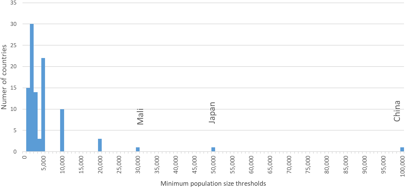
A specific population size threshold is mentioned for 100 countries in that methodological annex. The vast majority (85%) of these use a population threshold of 5 000 inhabitants or less (see Fig. 1). The most common thresholds are 5 000 (27 countries) and 2 000 (24 countries) Japan and China are outliers with thresholds that are ten to twenty times higher, respectively 50 000 and 100 000. For a good overview of how this has changed over time see [5]
Figure 1.
Population size thresholds to define urban population. Source: UN World Urbanization Prospects 2018.
The impact of a population size threshold to define an urban area depends on the size of the spatial units used. If spatial units cover a large area, they will have larger populations than if they covered only a small area. As a result, in countries with spatial units with a small area, more units would fall below the minimum population size threshold than in countries with large spatial units. Even spatial units that cover a small neighbourhood in a city, could fall below the minimum population size and thus be classified as rural. If the spatial units cover a large in area, many will exceed the minimum population threshold and be classified as rural, even if there are no large settlements within that area. This statistical distortion linked to the shape and scale of the spatial unit is a classic problem known as the modifiable areal unit problem [6].
Population density is highly sensitive to the area size of the spatial unit. Everything else being equal, large spatial units have lower population densities than small ones. This is probably why relatively few countries use this indicator. Only 17 countries reported using density as a criterion. For 10 countries, the actual density threshold is reported. In these countries, the population density varies from 150 inhabitants per km
2.2Municipalities, localities and settlements
The lack of consistent data with a high spatial resolution is a big obstacle to defining cities and settlements. The UN census recommendations underline that localities should not be equated with the smallest spatial units because a spatial unit can contain multiple small localities and a big locality can be spread across multiple spatial units.
Localities as defined above should not be confused with the smallest civil divisions of a country. In some cases, the two may coincide. In others, however, even the smallest civil division may contain two or more localities. On the other hand, some large cities or towns may contain two or more civil divisions, which should be considered as segments of a single locality rather than separate localities. [para 2.79] [7]
In other words, settlements (or localities) should be defined independently from civil or administrative divisions. For example, Finland defines an urban area as a population settlement of at least 200 inhabitants, where the distance between residential buildings is no more than 200 meters.22 In this definition, the first step is to create clusters of residential buildings and only then to count population. It does not directly measure the clustering of population, because historically the data on buildings had a higher spatial resolution than the population. A cadastral map with the outline of each building has a spatial resolution of a few meters, while the resolution of population data varied with the size of spatial units that had ranged from less than one square kilometer to several thousand square kilometers.
The UN recommendation defines a locality as a distinct population cluster [para 2.78] [7]. If the exact location of the population is known, there is no need to measure the distance between residential buildings to map population clusters. With growing use of geo-coded censuses – geo-referenced population registers, the accuracy of population data is much higher which then allows the direct identification of population clusters.
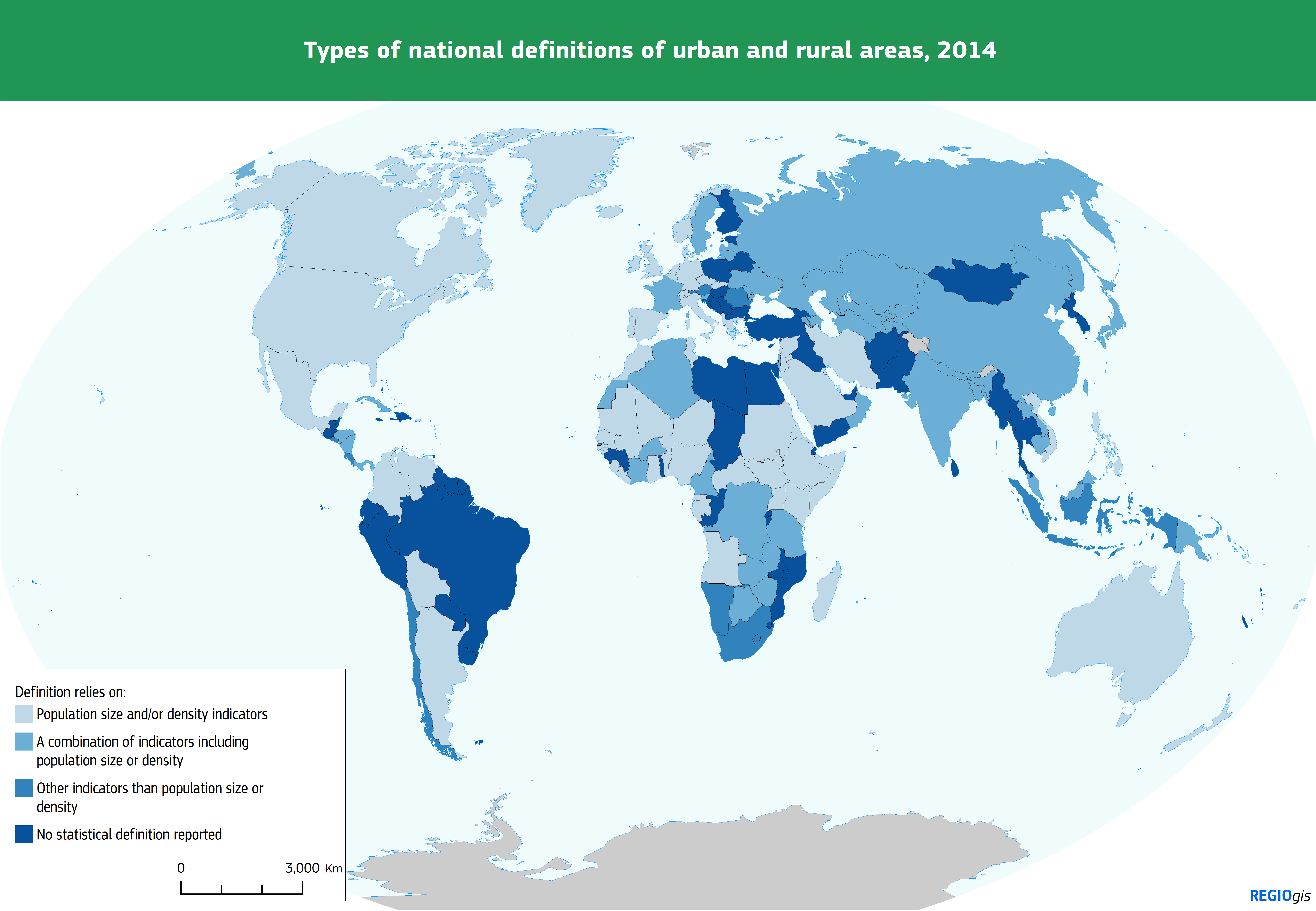
Figure 2.
Types of national definitions of urban and rural areas, 2014. Source: UN World Urbanization Prospects 2018.
2.3Definitions relying on administrative designation
About half (114 out of 233) of the definitions described in the methodological annex use an administrative designation, either exclusively or in combination with other indicators (see Fig. 2). For international comparisons, the drawback of using administrative designations is that they are country specific. They cannot be replicated in other countries. As a result, it is difficult to assess how similar or different these designated areas are.
Administrative designations vary widely. Some list a number of local authorities, as for example Trinidad and Tobago do. Some use an administrative rule. Brazil, for example, requires that every municipality or district, no matter how small, have an administrative centre that is defined as urban. Other countries combine an administrative designation with a more statistical definition. For example, Zimbabwe’s definition includes places that are simply designated as urban and places that are selected based on statistical indicators (minimum population of 2,500 inhabitants residing in a compact settlement pattern and where more than 50 per cent of the employed persons are engaged in non-agricultural occupations).
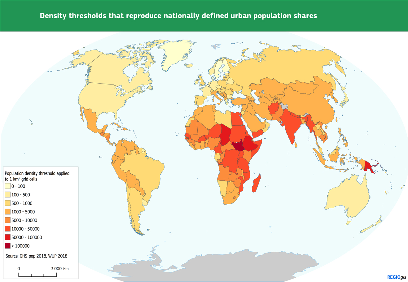
Figure 3.
Population density thresholds that reproduce nationally defined urban population shares, 2015. Source: UN World Urbanization Prospects 2018.
2.4Other criteria: Agricultural employment, infrastructure and services
Three other requirements appear frequently in urban and rural definitions: agricultural employment (37 definitions), certain types of infrastructure (19 definitions) and certain services (17 definitions). The biggest drawback of such definitions is that they can interfere with the relationship between on the one hand urbanisation and on the other hand economic development, access to infrastructure and services (see below).
2.5Empirical evidence that the national definitions are radically different
To verify if the different national definitions implicitly share a similar underlying concept, we measured what population density threshold applied to a population grid reproduces the same share of urban population that applying the national definition would yield. This makes a relatively plausible assumption that urban areas are denser than rural areas. The USA and India use a similar minimum population size threshold (2,500 and 5,000 respectively) to define urban areas [8]. According to the national definition, 82% of population in the USA lives in an urban area, 82% of the population also lives in 1 km
A general pattern emerges from this analysis. In the Americas, Europe and Oceania a relatively low population density threshold captures the same population share as the nationally defined urban population. In most countries in Africa and Asia, a higher population density threshold is needed to capture the same population share as the national urban definitions do. We have also tested this using larger grid cells (2 by 2 km, 5 by 5 km and 10 by 10 km) and the same pattern holds: To capture the same population share as the national urban definitions do, substantially higher population density thresholds are needed in Africa and Asia than in the Americas, Europe and Oceania.
This first test applied a density threshold to individual cells. We conducted a second test using a minimum population density thresholds applied to individual cells and a minimum population size applied to the clusters of contiguous cells above that density threshold. This means that first, all the cells above the population density threshold are selected. Next, all the cells above that threshold are clustered based on contiguity and the population of those clusters is calculated. Finally, all the cells in a cluster with a population below the minimum population size threshold are discarded. A wide range of combinations of population density and size thresholds were tested to identify which combinations reproduced the nationally defined urban population share. In the Americas, Europe and Oceania combinations of low population density and small population size thresholds reproduced the nationally defined urban population share, while in Africa and Asia combinations of high population density and large population size thresholds reproduced the national shares. These indicates that national definitions differ significantly and are less suitable for international comparisons. It also implies that a harmonised definition based on population size and density will in some countries lead to a big difference in the urban population share as compared to the nationally defined share.
One possible explanation for these differences could be that in countries split the urban-rural continuum in different ways. If we define the urban-rural continuum as going from large to small settlements, it could be that some countries only include large settlements in their urban category, while others also include medium-sized settlements in their urban category.
3.The degree of urbanisation to the globe
This section explains the benefits of the new method and provides a short overview of its main elements. The full detail of how to apply the method can be found in the dedicated manual [9].
The Degree of urbanisation (DEGURBA) is a classification that indicates the character of an area. It combines population size and population density thresholds to capture the complete hierarchy of settlements. A population grid of 1 km
3.1Benefits of the degree of urbanisation
There are six clear advantages of the new methodology.
• The Degree of Urbanisation captures the urban-rural continuum in three and seven classes. A growing number of countries uses more than two classes in an attempt to capture the urban-rural continuum. For example, India, the USA, Portugal and South Africa all uses three classes.
• While national definitions use very different population size and density thresholds, the Degree of Urbanisation classification uses the same thresholds across the globe.
• The Degree of Urbanisation avoids the distortions generated by spatial units that differ in shape and size, known as the modifiable areal unit problem. By starting with a classification of a 1 km
• It measures population clusters directly instead of a through a proxy. The United Nations Principles and Recommendations for Population and Housing Censuses [10] defines a locality or settlement as a distinct population cluster [Section 1.8, p. 187]. In the past, however, it was not possible to measure where people were clustered, while buildings were often mapped at a much higher spatial resolution than the population. Therefore, some national and academic definitions used clusters of buildings to identify settlements. Today, however, far more precise information is available on the distribution and location of populations. As a result, it is no longer necessary to approximate a population cluster by using a cluster of buildings. Measuring population concentrations directly makes them more comparable across different levels of (economic) development and over time.
Table 1
Short and technical terms for classifying small spatial units to levels 1 and 2 of the Degree of Urbanisation
Level Short terms Technical terms 1 Cities Densely populated areas 2 Cities Large settlements 1 Towns & semi-dense areas Intermediate density areas 2 Dense towns Dense, medium settlements 2 Semi-dense towns Semi-dense, medium settlements 2 Suburban or peri-urban areas Semi-dense areas 1 Rural area Thinly populated areas 2 Villages Small settlements 2 Dispersed rural areas Low-density areas 2 Very dispersed rural areas or Very low-density areas Mostly uninhabited areas • Defines areas to monitor access to services, not areas defined by access to services. The sustainable development goals include multiple indicators that monitor access to services or infrastructure. Examples include indicators measuring access to electricity, safely managed drinking water, a mobile phone network and all-weather roads. To properly monitor access to these services in urban and rural areas, these indicators should not be part of the definition. Take for example, a definition of an urban area that includes a criterion that everyone should have access to electricity. This would mean that some large and dense settlements without full access to electricity would be classified as rural and not urban. It would also make it impossible to monitor the access to electricity in urban areas as all urban areas would have access to electricity, because it is part of the definition of the urban area.
• This method is highly cost-effective. A population grid can be created for a relatively low cost using existing data. Compiling statistics by Degree of Urbanisation can often be done by re-aggregating existing data.
3.2The degree of urbanisation level 1 and level 2
The Degree of Urbanisation is applied in a two-step process: First, grid cells of 1 km
Classifying grid cells [9]:
• An urban centre or high density cluster is a cluster of contiguous cells of 1 km
• An urban cluster (moderate-density cluster) is a cluster of contiguous grid cells of 1 km
• Rural grid cells (mostly low-density cells) are the cells that are not identified as urban centres or as urban clusters. The vast majority of these cells have a density below 300 inhabitants per km
Classifying small spatial units:
Once grid cells have been classified, they can be overlaid to small spatial units yielding the level 1 of degree of urbanisation. A small spatial unit can be either an administrative unit or a statistical area. They are classified as following:
• Cities (or densely populated areas) are small spatial units that have at least 50% of their population in urban centres;
• Towns and semi-dense areas (or intermediate density areas) are defined as small spatial units that have less than 50% of their population in urban centres and no more than 50% of their population in rural grid cells;
• Rural areas (or thinly populated areas) are small spatial units that have more than 50% of their population in rural grid cells.
Urban areas are defined as cities plus towns and semi-dense areas, but as cities differ from towns and semi-dense areas, it is recommended to report on all three classes separately.
Changes to the classification of a given small spatial unit due to a change in the population distributions tend to occur only slow. As a result, updating the Degree of Urbanisation based on a new population grid may only be needed every 5 or 10 years.
The extensions to level 2 of the Degree of Urbanisation provide additional useful insight into the spatial structure of a territory or a country. Cities are clearly defined settlements, which can be organised by population size. The class of towns and semi-dense areas include towns and separate them in dense towns, semi-dense towns and suburban or peri-urban areas. Furthermore, rural areas are separated in villages, dispersed rural areas and mostly uninhabited areas. Level 2 classification is implemented in the same manner as level 1 classification.
The population density thresholds have specific terms; dense means at least 1500 inhabitants per km
The terms large, medium and small each refer to a specific population size threshold: large means a population of at least 50 000 inhabitants, medium means a population of at least 5 000 inhabitants and small means a population between 500 and 4 999 inhabitants. The technical terms for small spatial units that refer to a city, town or village include the word ‘settlement’, while the others use the word ‘area’.
3.3Functional urban areas or metropolitan areas
Functional Urban Areas (FUAs) can complement the Degree of Urbanisation classification. A FUA or metropolitan area is composed of a city plus its surrounding, less densely populated spatial units that make up the city’s labour market, its commuting zone. The FUAs and the Degree of Urbanisation classification are linked by usage of the same exact concept of city. FUAs can be defined as follows; identifying an urban centre, followed by overlaying small spatial units that have at least 50% of their population in an urban centre-which identifies the city. A commuting zone is then identified as a set of contiguous small spatial units that have at least 15% of their employed residents working in a city.
4.Comparing population in cities, urban and rural areas using national definitions and the Degree of Urbanisation
This section compares the population shares as defined by the Degree of Urbanisation with the data published by the UN DESA Population Division in the World Urbanization Prospects [1] based on national definitions. To estimate population share by Degree of Urbanisation, this method was applied to a global, open and free population grid.44 The population grids combine census-based population data collected by CIESIN at Columbia University (GWPv4.10) [11] with grids reporting built-up densities [12].
First, we compare nationally defined cities-and urban centres (cities) based on two above-mentioned sources with at least 300 000 inhabitants Second, we compare the share of population in urban and rural areas.55
4.1Population shares in large cities are similar between the national and global definition
The global population living in cities of at least 300,000 based on national definitions is identical to that based on the Degree of Urbanisation. The World Urbanization Prospects [1] lists 1,772 cities with at least 300,000 inhabitants in 2015 compared to 1,773 cities as defined by the Degree of Urbanisation.66 Both account for 31% of the global population. This high level of agreement may be because large cities are relatively easy to define. These dense large urban settlements are typically known to everyone in a country.
Some variation can still be observed between the different geographical regions of the world. The national definitions yield slightly higher population shares in Europe and the Americas and in some cases lower shares in Africa and Asia as compared to the Degree of Urbanisation definition (see Fig. 4).
Figure 4.
Population in cites with over 300,000 inhabitants using the Degree of Urbanisation and national definitions, 2015. Source: UN World Urbanization Prospects 2018.
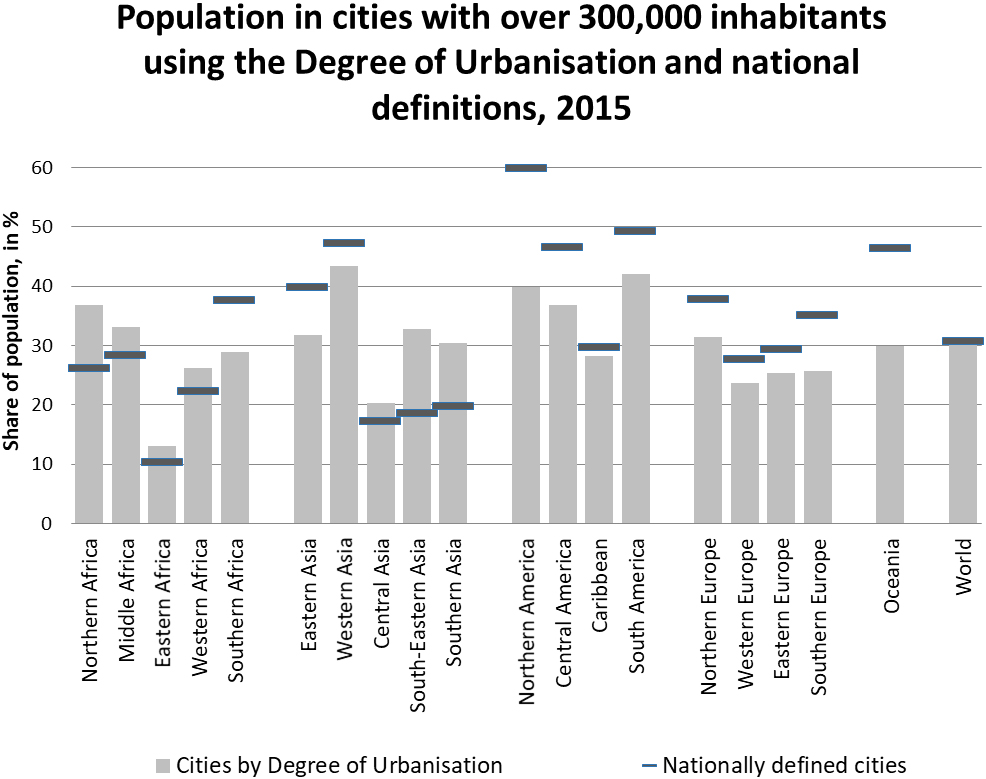
Figure 5.
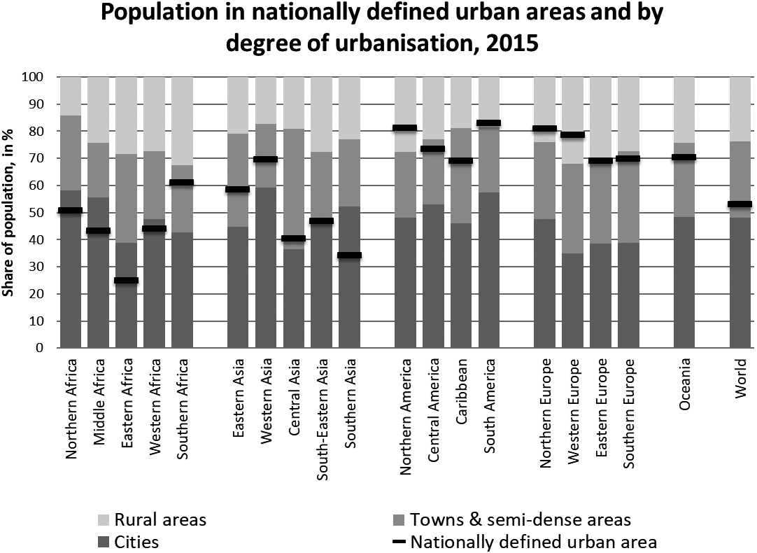
Population by Degree of Urbanisation and nationally defined urban areas, 2015. Source: UN World Urbanization Prospects 2018.
One conceptual difference is apparent in these figures-the population share in cities over 300,000 based on national definitions is considerably higher in North America and Oceania (60% vs 38% and 49% vs 30%). This is because these countries report data for ‘urban agglomerations’ which are defined as a city and its contiguous suburbs. While the data based on the Degree of Urbanisation only considers the city population. Comparing these national defined urban agglomerations to the functional urban areas or metropolitan areas shows a much higher level agreement.77
4.2Rural population shares vary between the national and global definition
The population shares in the nationally defined rural areas are quite similar to the rural areas as defined by the Degree of Urbanisation in the Americas, Europe and Oceania (see Fig. 5). In Africa and Asia, the population share in nationally defined rural areas is much larger than in the rural areas as defined by the degree of urbanisation. In most cases, it is closer to the population share in cities as defined by the degree of urbanisation. This big difference in the rural population share may be due to conceptual differences in the rural definition. For example, national rural definitions in Africa and Asia may include medium-sized settlements, while national rural definitions exclude medium-sized settlements in the America, Europe and Asia. For example, Japan and China use a minimum urban population threshold of 50 000 and 100 00, compared to 200 and 2 500 in Denmark and France.
The estimated population grid (GHS-POP) used for these calculations is based on population data that typically has a coarser spatial resolution in Africa and Asia compared to the Americas, Europe and Oceania. This may have led to an underestimation of the rural population in Africa and Asia. Improving the estimated population grids and grids based on geo-located censuses in these regions can help to assess the extent of this potential underestimation.
5.Conclusions
This article argues that national definitions of urban areas are too different among each other to be used for international comparisons. For instance, the minimum settlements sizes ranging from 200 inhabitants (Denmark) to 100 000 (China). The three main reasons why they are too different are: 1) Half the countries rely on an individual administrative designation, which cannot be replicated; 2) The other half do use a statistical definition but many rely on indicators that are either not available for all countries or not suitable for a global definition; and 3) the countries that use a minimum population size use quite different thresholds and apply them to units of very different shapes and sizes.
Tests showed that the population shares in nationally defined urban areas could not be replicated using the same population density and size criteria globally. In the Americas, Europe and Oceania a low population density and size thresholds could replicate the national shares, while in Africa and Asia high population density and size thresholds were typically needed. This suggests that some countries use ‘urban areas’ to refer exclusively to large settlements, while others use it to refer to large and medium-sized settlements.
Estimates indicate that the population shares in cities of 300 000 inhabitants or more as defined by the degree of urbanisation are very similar to the share based on nationally definitions. This suggests that national definitions and the Degree of Urbanisation agree on how to define a large city. Population shares in rural areas as defined by the Degree of Urbanisation and in nationally defined rural areas are very similar in the Americas, Europe and Oceania, but very different shares in Africa and Asia. This could be because urban areas in Africa and Asia typically only refer to larger settlements, while medium-sized settlements are included in the rest of the world.
We hope that in the coming years more countries will apply the Degree of Urbanisation and produce the SDG indicators using the Degree of Urbanisation. This would allow statistical comparability on the international level. The European Commission and UN-Habitat offer online support and hands-on training to facilitate this process.
Notes
3 The second step of this method classifies administrative or statistical spatial units, which reintroduces the problem of working with units of varying shapes and sizes. Therefore, it is recommended to use small administrative or statistical spatial units; this should ensure a good match with the grid classification. Applying this method to very large units, such as regions, may significantly alter population shares when compared with the grid classification.
5 Please note that all the data presented here is only at the grid level. Unfortunately, it was not possible to obtain a global layer with all the census enumeration areas or other small spatial units. Therefore, the data here only covers the first step of the degree of urbanisation: i.e. the coding of the grid cells. For ease of reading, the terms for the spatial units are used here, although the data refers to the grid cell concepts. Finally, we show the results using an alternative global population grid to test the impact of the assumptions needed to create a global population grid.
6 The cities included in this comparison have been manually validated. Urban centres that were judged to not represented a city or were not certainly representing a city were excluded from this comparison. As a result, the population in urban centres reported here is slightly lower than in the previous section (45% instead of 48%). Most of the urban centres that were excluded can be found in Middle and Eastern Africa, Southern Asia and Oceania.
7 Metropolitan areas tend to be large than urban agglomeration because a commuting zone can extend beyond the suburbs and also include some of the surrounding rural areas.
References
[1] | World Urbanization Prospects 2018 – Population Division – United Nations [Internet]. UN DESA. (2018) [cited 9 April 2018]. Available from: https://esa.un.org/unpd/wup/. |
[2] | Gross M. The urbanisation of our species. Current Biology. (2016) ; 26: (23): R1205–R1208. doi: 10.1016/J.CUB.2016.11.039. |
[3] | Melchiorri M, Florczyk AJ, Freire S, Schiavina M, Pesaresi M, Kemper T. Unveiling 25 years of planetary urbanization with remote sensing: Perspectives from the global human settlement layer. Remote Sens. (2018) ; 10: (5): 768. |
[4] | Freire S, MacManus K, Pesaresi M, Doxsey-Whitfield E, Mills J. Development of New Open and Free Multi-temporal Global Population Grids at 250 m Resolution. Proceedings of the 19th AGILE Conference on Geographic Information Science, 2016 June 14–17, Helsinki. |
[5] | Buettner T. Urban estimates and projections at the united nations: The strengths, weaknesses, and underpinnings of the world urbanization prospects. Spatial Demography. (2015) ; 3: : 91–108. doi: 10.1007/s40980-015-0004-2. |
[6] | Gehlke C, Biehl K. Certain effects of grouping upon the size of the correlation coefficient in census tract material. Journal of the American Statistical Association. (1934) ; 29: (185): 169. |
[7] | United Nations Statistics Division – Demographic and Social Statistics [Internet]. Unstats.un.org. (2022) [cited 15 April 2022]. Available from: https://unstats.un.org/UNSD/Demographic/sconcerns/densurb/densurbmethods.htm. |
[8] | U.S. Census Bureau. Urban area criteria for the 2010 census. Fed. Regist. (2011) . |
[9] | Applying the degree of urbanisation. European Union/ FAO/UN-Habitat/OECD/The World Bank; (2021) . |
[10] | Principles and recommendations for population and housing censuses. New York: United Nations; (2017) . |
[11] | Center for International Earth Science Information Network. Urban Extents Grid, v1: Global Rural-Urban Mapping Project (GRUMP), v1 |
[12] | Freire S, Schiavina M, Florczyk A, MacManus K, Pesaresi M, Corbane C, et al. Enhanced data and methods for improving open and free global population grids: Putting ‘leaving no one behind’ into practice. International Journal of Digital Earth. (2018) ; 13: (1): 61–77. |
[13] | Angel S, Parent J, Civco DL, Blei AM. Making room for a planet of cities, Lincoln Institute of Land Policy. (2011) . doi: 10.4337/9781849808057.00023. |
[14] | Balk DL, Deichmann U, Yetman G, Pozzi F, Hay SI, Nelson A. Determining global population distribution: Methods, applications anghd data. Advances in Parasitology. (2006) ; 62: : 119–156. |
[15] | Corbane C, Pesaresi M, Politis P, Syrris V, Florczyk AJ, Soille P, Maffenini L, Burger A, Vasilev V, Rodriguez D, Sabo F, Dijkstra L, Kemper T. Big earth data analytics on Sentinel-1 and Landsat imagery in support to global human settlements mapping. Big Earth Data. (2017) ; 1: : 118–144. doi: 10.1080/20964471.2017.1397899. |
[16] | Esch T, Marconcini M, Felbier A, Roth A, Heldens W, Huber M, et al. Urban footprint processor – fully automated processing chain generating settlement masks from global data of the TanDEM-X mission. IEEE Geosci. Remote Sens. Lett. (2013) ; 10: : 1617–1621. doi: 10.1109/LGRS.2013.2272953. |
[17] | Forstall RL, Greene RP, Pick JB. Which are the largest? Why lists of major urban areas vary so greatly. Tijdschrift Voor Economische En Sociale Geografie. (2009) ; 100: (3): 277–297. |
[18] | Statistics and databases [Internet]. International Labour Organization. (2022) [cited 9 May 2018]. Available from: https://www.ilo.org/global/statistics-and-databases/lang–en/index.htm. |
[19] | Kuhn TS. The Structure of Scientific Revolutions, University of Chicago Press. (1970) . doi: 10.1119/1.1969660. |
[20] | Openshaw S. Ecological Fallacies and the Analysis of Areal Census Data. Environ. Plan. A. (1984) . doi: 10.1068/a160017. |
[21] | Pesaresi M, Huadong G, Blaes X, Ehrlich D, Ferri S, Gueguen L, et al. A global human settlement layer from optical HR/VHR RS data: Concept and first results. IEEE Journal of Selected Topics in Applied Earth Observations and Remote Sensing. (2013) ; 6: (5): 2102–2131. doi: 10.1109/jstars.2013.2271445. |
[22] | Pesaresi M, Syrris V, Julea A. A new method for earth observation data analytics based on symbolic machine learning. Remote Sensing. (2016) ; 8: (5): 399. |
[23] | Uchida H, Nelson A. Agglomeration Index? Towards a New Measure of Urban Concentration. (2009) . |


