
Small area estimation of non-monetary poverty with geospatial data
Abstract
This paper evaluates the benefits of combining household surveys with satellite and other geospatial data to generate small area estimates of non-monetary poverty. Using data from Tanzania and Sri Lanka and applying a household-level empirical best (EB) predictor mixed model, we find that combining survey data with geospatial data significantly improves both the precision and accuracy of our non-monetary poverty estimates. While the EB predictor model moderately underestimates standard errors of those point estimates, coverage rates are similar to standard survey-based standard errors that assume independent outcomes across clusters.
1.Introduction
A proliferation of geospatial data obtained from satellites and mobile devices – as well as research demonstrating that satellite and mobile phone records are strongly correlated with household welfare – has sparked great interest in statistical methods that combine this geospatial data with survey data [1, 2, 3, 4, 5]. A key motivation for complementing survey data with comprehensive geospatial data is the potential for small area estimation, which can produce more precise and granular estimates of socioeconomic indicators. Geospatial data are well-suited for this application because, like a census, they are geographically comprehensive and not subject to selection bias. Established methods for small area estimation typically use either “unit-level” or “area level models”, depending on the availability of household-level auxiliary data. Unit-level models in practice typically utilize household survey data and contemporaneous household census data, by first estimating a prediction model of household welfare in the survey data and then using the estimated model parameters to simulate welfare in the census [6, 7, 8]. Simulations of household welfare are then aggregated to the target area level. Because this method relies on census data, however, strong assumptions are typically required to use survey data to update estimates in the absence of a census.11 Census data are typically dated and collected once per decade at best, which presents a significant hurdle to deriving timely small area poverty estimates.
To overcome these challenges, we link census data with geospatial and remote-sensing auxiliary data at the village level.22 Village in this case refers to the lowest geographic level at which spatial auxiliary data can be merged with household surveys containing data on welfare and poverty. Meanwhile, small area refers to the target level for the poverty estimates. Finally, regions are the lowest level for which the household budget survey is representative. In recent household surveys, GPS coordinates of households, enumeration areas, or villages are often available, which allows analysts to link survey data with other auxiliary sources of remote-sensing or geospatial data and improve the precision of poverty estimates.
The exact locations of survey respondents are guarded very closely by statistical agencies to preserve anonymity. However, village IDs or the location of enumeration areas can be obtained in some cases, enabling the survey to be linked to auxiliary data at the EA or village level. Linking surveys with geographically aggregated auxiliary data, whether derived from census or geospatial sources, is less efficient than using household-level data from a census. On the other hand, it also offers the key benefit of being able to include the auxiliary data directly in the prediction model. This is typically not feasible when using census data at the household level, because of the confidentiality concerns associated with linking survey data with census data for individual households. Therefore, unit-level models using census auxiliary data typically use variables common to the census and survey and assume that these prediction variables are drawn from the same underlying distribution, which in turn becomes problematic when there is a large time gap or are differences in questions between the census and the survey.
Using geospatial auxiliary data in particular offers further advantages, in that spatial auxiliary data are collected continuously, eliminating any concerns about a time gap between survey and auxiliary data, and are highly predictive of village level poverty. Both the quality and availability of geospatial data are improving rapidly. Finally, geospatial data is geographically comprehensive and representative, as opposed to mobile phone data which often represents only a portion of the population and is more difficult to obtain.
While there are many studies seeking to predict welfare, poverty or other development outcomes with a combination of survey data and geospatial data [1, 2, 4, 13, 14, 15], only a few have evaluated and quantified the gain in the precision of small area estimates achieved by supplementing survey data with geospatial data.33 This study uses data from Sri Lanka and mainland Tanzania to assess the feasibility of combining traditional household survey with satellite and remote-sensing data to improve the precision and accuracy of small area estimates of non-monetary poverty.44 These two countries were selected due to the availability of census data with geo-referencing information that can be matched with spatial features at the village level, which in this context refers to GN Divisions in Sri Lanka and villages in Tanzania.55 The proposed welfare prediction model uses survey data to estimate household welfare as a function of village characteristics, and therefore differs from standard small area estimation models that predict welfare using a mix of household and small area characteristics. The resulting estimates provide a large efficiency gain compared with estimates solely based on the household survey, which we refer to as direct survey estimates.
We mainly consider Empirical Best Predictor (EBP) models, which have a long history in small area estimation and can accommodate village-level auxiliary data to produce estimates of poverty rates and their mean squared error for small areas. When auxiliary data is aggregated at a geographic level such as a village, EBP models have an important advantage over alternative methods, such as the ELL method [6] and the “M-quantile” method [16] because it conditions on and therefore effectively combines household level survey data with village-level auxiliary data. Empirical evidence that EBP is far more efficient than ELL in this context is discussed below, in section 5.66 When using household- level auxiliary data, ELL can outperform EBP in terms of relative bias and relative root mean squared error in certain situations [17].
We compare the estimates generated by a household EBP model with direct estimates obtained solely from the survey, as well as the well-known Fay-Herriot area-level model [18]. The latter sacrifices precision by discarding the variation in the geospatial indicators across villages within small areas. Once the small area estimates are obtained from the household EBP and Fay-Herriot models, we compare them to non-monetary poverty rates calculated directly from the full census. The availability of census data provides a credible benchmark to establish the feasibility of the method and assess how different methods and their variants perform, in terms of the accuracy of both the small area point estimates and their confidence intervals. We compare the predictions from different methods in terms of their precision, their accuracy, and their coverage rate. The coverage rate is defined as the share of small areas for which the estimated 95 percent confidence intervals for the small area non-monetary poverty rate contains the census non-monetary poverty rate.
The main result is that incorporating remote sensing data in an EBP framework substantially improves the accuracy and precision of small area estimates of non-monetary poverty relative to direct survey estimates. While the main efficiency improvements occur by incorporating information from non-sampled villages, there are also minor efficiency improvements from combining sample data with synthetic predictions in sampled villages. This comes at no cost to coverage rates in Sri Lanka and a moderate cost in Tanzania, compared with standard direct survey estimates. The corresponding efficiency improvement is comparable to approximately tripling the size of the survey in Sri Lanka and quintupling it in Tanzania.
EBP is an appealing framework in this context because it has become a popular and widely accepted method, and is straightforward to apply in well-documented software. However, it does in this context moderately underestimate mean squared error, for two reasons. First, the EBP estimator fails to account for uncertainty in estimated variance parameters from the model. Second, when conditioning on the sample, the EBP estimator incorrectly assumes that sample observations are independent within small areas. Estimated coverage rates remain respectable, however, at 75 percent in Tanzania and 84 percent in Sri Lanka when the small area estimates are calibrated to ensure that their regional estimates match with those derived from the household survey.77 This is comparable to the 76 percent coverage rate in both countries when using standard direct estimates. In Tanzania, the estimates from the unit level model are roughly as accurate and moderately more efficient than those from the area-level Fay-Herriot model. In Sri Lanka, where the poverty rate is low and the Fay-Herriot model is less predictive, the estimates from the unit-level model are substantially more accurate and efficient than the small area level Fay-Herriot estimates.
These results hold under a variety of robustness checks that explore alternative implementation options, including the omission of sample weights and a different transformation method in EBP, the application of a different model selection algorithm as well as the absence of benchmarking to survey estimates at higher levels and the use of a noisier welfare measure. As a robustness check, we also test how EBP performs vis-à-vis the other most commonly used unit-level model ELL and show that EBP estimates are much more efficient than ELL estimates. When using the noisier welfare measure, the gain in efficiency is not as large in Sri Lanka, on the order of doubling the size of the sample, but the predictions remain accurate and coverage rates remain high.
This study makes three main contributions. First, it applies a commonly-used framework for small area estimation to combine household survey data on well-being with geographically comprehensive geospatial indicators at a national level. To our knowledge, it is the first paper that applies the EBP framework to geospatial data outside of the 12 Iowa countries studied in [13]. Second, it evaluates the extent to which incorporating geospatial variables at the subarea level improves the precision of small area poverty estimates, compared with direct survey estimates. Finally, it assesses which of two commonly used SAE models – unit-level models [6, 8, 21], and the Fay-Herriot area-level model [18] – are best suited for combining survey and sub-area geospatial data to produce efficient and accurate estimates of both area-level poverty rates and the uncertainty associated with them. The results taken together demonstrate that augmenting survey data with publicly available geospatial data enhance the accuracy and precision of small area estimates, and that unit-level models are preferred to area-level models when geospatial data is available at the sub-area level.
The remainder of the paper is organized as follows. Section 2 describes the data. Section 3 describes the methodology and estimators that are evaluated. Section 4 assesses results in terms of efficiency, accuracy, and coverage. Section 5 considers a variety of robustness checks of the main method. Section 6 concludes.
2.Description of the data
2.1Constructing measures of non-monetary welfare and poverty in the census
The first step of the analysis is to construct measures of non-monetary poverty based on the Sri Lankan and Tanzanian censuses, which were each conducted in 2012. Non-monetary poverty, unlike monetary poverty, is directly observed in the census population and can therefore provide a benchmark for evaluation. For each country, we identified a set of household assets (e.g., ownership of TVs, computers, housing materials) and demographic proxies (e.g., gender of household heads, household size, literacy, sector of work) for welfare. We then carried out a principal component analysis, weighted according to household size, to estimate a loading factor for each proxy welfare indicator.88 The principal component analysis is based on the correlation matrix, weighted by household size, and the first principal component was retained. Each household’s non-monetary welfare measure was obtained by summing the product of each loading factor and the household’s value of the associated variable. We then set a poverty threshold at the 4
2.2Constructing synthetic household surveys
The previous section discussed the measure of non-monetary welfare and poverty, defined as the share of the population for which the non-monetary welfare measure is below the respective poverty line for Sri Lanka and Tanzania. With these in hand, we turn to drawing a synthetic household survey from each country’s census. The synthetic survey, along with the auxiliary geospatial data, are key inputs into the small area estimation procedures. To draw the synthetic survey, we utilized the actual two-stage sample conducted by the National Statistics Offices for two household budget surveys: The 2018 Tanzania Household Budget Survey, and the 2016 Sri Lanka Household income and Expenditure Survey. These surveys were merged with the census at the village level, which is the GN Division in Sri Lanka and the village in Tanzania1010 After retaining the GN Divisions and EAs present in the household survey, we randomly selected census households in each matching EA to match the number of households in each EA for each survey. Finally, we merged the sample weights from the household budget surveys for each village. Essentially, this procedure drew synthetic surveys that mimicked as much as possible the sample drawn by the NSO for the household surveys.
2.3Remote sensing data
The auxiliary data for the small area estimation exercise were drawn from a large candidate pool of satellite-derived information. Most of these geospatial data are derived from publicly available layers and imagery, including, but not limited to, night-time lights from the Visible Infrared Imaging Remote Sensor (VIIRS); precipitation data from the Climate Hazards Group InfraRed Precipitation with Station data (CHIRPS) and [22]; elevation and slope taken from [23] and the Advanced Spaceborne Thermal Emission and Reflection Radiometer (ASTER) satellite; global forest cover change from [24] estimates of built-up area from the Global Human Settlement Layer (GHSL), population estimates (WorldPop); climactic region1111 from [25]; and lastly, crop yield estimates for Maize, Sorghum, and Rice [26].1212
The Sri Lanka indicators were also supplemented by a variety of spatial “contextual” features derived from a cloud-free mosaic of 2017–2018 Sentinel-2 imagery, which is collected every 5 days by Sentinel 2 sensors on board two satellites, Sentinel 2A and 2B.1313 These contextual features have been shown to be strongly correlated with poverty, population density and building and road characteristics [4, 33, 34]. These contextual features were calculated by comparing pixels with their neighbors and then reporting this value back to the individual pixel (in this case 10m). The number of neighboring pixels considered in the comparison is the scale, which varies by the feature being calculated.1414 Since these contextual features are derived from Sentinel 2, they are available at 10 m spatial resolution and are theoretically available for free for the entire world. Cloud free Sentinel 2 mosaics can be made in Google Earth Engine and the code to calculate the contextual features is written in Python (SpFeas package). Therefore, all that is required to calculate the features is computer processing time. While the majority of remote sensing data used for Tanzania were largely derived from publicly available imagery, it was supplemented by proprietary data on building footprints produced by Ecopia and Maxar based on very fine spatial resolution imagery.1515 While these data are more costly and difficult to create than the contextual features, with these data we are able to capture the spatial patterns of buildings and roads, their density, and the general neighborhood structure that is indicative of relative differences in poverty over space [4, 33]. The building footprint data was proprietary when we first did this study and costly to create. However, the costs are rapidly decreasing as satellite imagery becomes cheaper, more ubiquitous and computing power becomes less expensive and recently Google released a similar data set covering the majority of the African continent.1616 Also, additional data sources such as Open Street Map are rapidly increasing in spatial coverage. Together, the open source nature of the contextual features, and the increasing availability of satellite derived data going forward, makes using these types of data in studies such as this in the future very feasible.
2.4Geographic structure of Sri Lanka and Tanzanias
Before describing the methodology used in the study, we briefly review the geographic structure of the two countries. Villages are the lowest level for which shapefiles were obtained and are therefore the most disaggregated level for which geospatial data could be linked with the survey. Small areas are the target domains for the small area estimates, which are at a higher level than the villages, but below the level at which the survey is considered to be representative. For Sri Lanka, there are 13,978 villages1717 (GN divisions), 331 areas (DS divisions), and 25 regions (districts); while Tanzania contains 14,981 villages, 159 areas (districts), and 25 regions.1818
3.Methods
This section describes the three methods that are evaluated: Direct survey estimates, the Fay-Herriot area-level model, and the household-level EBP model. It also discusses important methodological considerations involved when estimating the household-level model, such as differences between software packages, transforming the dependent variable, the model selection procedure, and benchmarking. The final subsection considers the criteria used to evaluate the performance of different estimators.
3.1Direct survey estimates
Direct estimates obtained from the survey serve both as a benchmark against which to assess the increase in precision from incorporating satellite data, and as an input into the Fay-Herriot area-level models. The most common method of obtaining variance estimates clusters the residuals by enumeration area, which accounts for positive correlation within clusters but assumes that disturbances across clusters are independent [35, 36]. As an alternative, we also applied the Horvitz-Thompson (H-T) approximation, which offers an alternative approach to estimate the variance of the small area poverty rates [37]. The H-T approximation also underestimates the variance, but in these contexts by less than clustered standard errors, and therefore yield less biased variance estimates. The H-T approximation underestimates the variance by assuming that the joint inclusion probabilities are the product of the marginal inclusion probabilities, which holds only for Poisson sampling.1919
3.2Fay-Herriot area-level model
The Fay-Herriot model was introduced by Fay and Herriot [18] to model incomes for small areas of fewer than 1,000 persons in the United States, and is perhaps the best-known and widely used small area-level estimator. It was derived as an application of the James-Stein estimator [38] using data aggregated to the small area level, and is also the Empirical Best Linear Unbiased Predictor (EBLUP) of the small area level regression. It is an “empirical” best linear unbiased predictor because the survey error variance is assumed to be known. The small area estimates are a weighted average of the synthetic regression prediction and the direct survey estimate, with the weights inversely related to the estimated variance of the direct and synthetic estimates. Many variants of the Fay-Herriot estimator have been developed that employ transformations and account for spatial and intertemporal correlation, among other refinements. We estimate a basic area-level Fay-Herriot model, using the Horvitz-Thompson approximation to calculate the variance of the direct survey estimate, as recommended by [39].
The Fay-Herriot estimator, unfortunately, has several limitations for the purposes of generating small area estimates of poverty using spatial auxiliary data. The main shortcoming is that the Fay-Herriot model requires aggregating the auxiliary data to the small area level, which discards variation in the auxiliary data at the village level that would increase the precision of the estimates. This is consistent with the strand of the small area estimation literature that emphasizes the importance of including cluster-level “auxiliary data” from censuses to control area-specific bias, reduce uncertainty, and estimate uncertainty more accurately [40, 41]. Implementing a sub-area model that adapts the Fay-Herriot model to address this issue, such as the one proposed by [42] can incorporate auxiliary data at the village level but is currently constrained by the lack of available software. Another limitation is that, because the Fay-Herriot model is based on direct estimate of poverty rates, it discards information on the variation in welfare within the poor and non-poor portions of the welfare distribution. In addition, when no transformation is applied, as is the case below, the poverty rate is assumed to be a linear function of the predictors, which can lead to predictions that are negative or greater than one. The Fay-Herriot model also faces challenges when no households are poor in a significant number of small areas, as is the case in Sri Lanka.2020 For these small areas, either the prediction from the auxiliary data must be ignored, the sample must be ignored, or they must be dropped from the estimation. Finally, the Fay-Herriot model does not account for uncertainty in the survey-based estimates of variance, which tends to underestimate the variance of the prediction.
Despite these limitations, the Fay-Herriot model is much simpler to apply and explain than a unit level model. It generally provides credible estimates and is a standard workhorse when using area level models for small area estimation. We estimate a Fay-Herriot model by aggregating all indicators to the small area level, weighting by population. The Fay-Herriot models are estimated using the Stata FHSAE command [43]. We utilize the “Chandra method”, which estimates the prediction model using Feasible Generalized Least Squares [44].
3.3Household-level model
In contrast to area level models, unit level models are specified at the level of the individual unit, which in this case is the household.2121 Although the auxiliary data only varies at the village level, predicting welfare at the household level fully utilizes the information in the sample survey on the level and variability of household welfare. Unit-level models are more convenient to estimate than sub-area models, because of the availability of well-established software packages that utilize empirical best methods with conditional random effects specified at the level of the small area.
The EBP model can be written as follows:2222
(1)
where
A key feature of the EBP framework is that the random small area effect
(2)
(3)
(4)
Where
(5)
is the shrinkage factor due to conditioning the random effect on the sample mean for small area
EBP estimation has proven to offer a large efficiency improvement compared to other methods such as the traditional ELL. This efficiency gain comes from the fact that the EB method conditions on the sample and thereby makes more efficient use of the information given, while ELL does not. When the auxiliary data are specified at an aggregate geographic level, such as a village or small area in the EBP framework described above, the use of predictors aggregated to the village level increases the variance of the small area effect
The assumption of normality is critical in the EBP framework, as a distributional assumption is required to condition the small area level random effect on the average residual of the regression in that small area. The normality assumption is consequently also necessary for the Monte-Carlo simulations of the parameters, which are required because headcount poverty is a non-linear function of welfare. Violations of the normality assumption can therefore lead to biased estimates. Below, we discuss a monotonic transformation to the welfare measure that makes the assumptions that the small area effect and the household error term are distributed normally more palatable.
3.4Normalizing transformation
Welfare typically follows a right-skewed distribution, and it is therefore standard practice to transform the welfare indicator before implementing small area estimation models based on simulated welfare. The most common transformation is to take the logarithm of welfare, following [6].2424 More recently, Box-Cox or Log-shift transformations h ave become more popular [47]. However, our preferred estimates utilize a monotonic transformation called the “ordered quantile normalization” to transform welfare, which transforms the scaled rank of the welfare variable to conform with a normal distribution. Among several methods proposed in the literature, the ordered quantile normalization most consistently transforms an underlying variable to follow a normal distribution [48]. While a normally distributed outcome variable does not guarantee normality of the residuals, in these cases it helps make the distribution of residuals closer to normal, and leads to smaller discrepancies between the official national poverty rate estimated from the survey and the weighted mean of the small area estimates.2525
3.5Model selection using Lasso
Model selection in small area estimation remains an unsettled issue and has traditionally been treated as both art and science.2626 In recent years, the least absolute shrinkage and selection operator (LASSO) has become an increasingly popular tool for selecting prediction models. The post-lasso procedure, in particular, offers the benefit of a convenient and data-driven approach to model selection that, in its most popular variant, maximizes out-of-sample predictive accuracy, while roughly equalizing in and out of sample R
3.6Benchmarking
Calibrating the small area estimates to match the direct sample estimates for regions can be desirable to ensure that the population-weighted average of small area poverty estimates, when aggregated to regions, match official published statistics derived from the survey [19, 20]. We therefore apply a simple ratio benchmarking procedure by multiplying the estimated headcount rate in each small area by a scaling factor unique to each region,2828 for both the Fay-Herriot and household level model estimates.2929 Below, we report results without benchmarking as a robustness check to assess whether and to what extent the procedure improves the accuracy of the estimates.
3.7Criteria for evaluating estimates
To evaluate the performance of the above-mentioned different SAE methods, we examine seven summary statistics, averaged across areas: non-monetary poverty rates; Mean Squared Error (MSE); Coefficient of variation (CV);3030 Relative Bias;3131 correlation between estimated and census non-monetary poverty rates; Root Mean Squared Error3232 (RMSE); and lastly coverage rate or the share of small areas for which the estimated 95 percent confidence intervals for the small area non-monetary poverty rate contains the census non-monetary poverty rate.3333
4.Main results
4.1Predictive power of geospatial variables
In both the area-level (Fay-Harriot) and unit-level (EBP) models, geospatial variables perform reasonably well in explaining variation in poverty or consumption. The small area-level predictor variables were selected using the lasso plugin method, to prevent overfitting the model to the sample. The set of candidate variables included all small area-level remote sensing indicators as well as regional dummies. For the Fay Harriot models, which is used as a reference point for comparison with the direct estimates and the unit level model, the lasso selected a small number of predictor variables, only 3 in Tanzania and 8 in Sri Lanka. Despite containing only three variables, the Tanzania model explains half of the variation in non-monetary poverty rates. Meanwhile, the eight Sri Lanka variables explain 6 percent of the variation in headcount poverty across subdistricts. Overall, the results suggest that the Fay-Herriot estimates, despite using predictors that only vary across small areas, can significantly improve on the efficiency of the direct estimates, particularly in Tanzania where the model fit is especially good.3434
Table 1
Details and diagnostics for unit level models
| Sri Lanka | Tanzania | |
| Poverty rate | 4.0% | 20.0% |
| Number of variables selected for model | 28 | 19 |
| Number of households in sample | 19,570 | 9,393 |
| Number of households out of sample | 4,190,436 | 8,901,279 |
| Number of villages in survey | 2487 | 786 |
| Number of villages in census | 13,985 | 14,981 |
| Number of areas in survey | 328 | 159 |
| Number of areas in census | 331 | 159 |
| Unit-level model diagnostics | ||
| Marginal R | 0.266 | 0.299 |
| Conditional R | 0.296 | 0.323 |
| Skewness of small area effect | 0.101 | |
| Kurtosis of small area effect | 3.385 | 3.60 |
| Wilks-Shapiro P-value | 0.558 | 0.316 |
| Skewness of household error | ||
| Kurtosis of household error | 3.23 | 3.51 |
| Variance of estimated small area effect | 0.036 | 0.024 |
| Variance of estimated household residual | 0.723 | 0.682 |
| Percentage of variance of error term due to small area effect | 5.0% | 3.5% |
Notes: Table reports number of selected variables, number of observations, number of villages and target small areas, conditional and marginal R
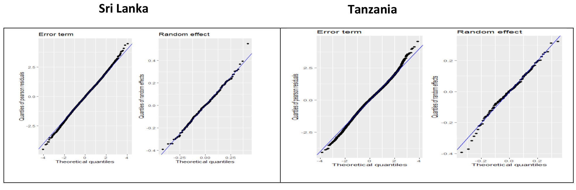
Figure 1.
Quantile vs. Quantile plots of household error terms and small area random effects. Notes: Figures report normal quantile-quantile plots of estimated household welfare residuals (error term) and small area random effects (random effect).
Turning to the results from the unit-level EBP models, the first striking result is the overall predictive power of the models. Tabke 1 summarizes the results from the model specifications employed for Sri Lanka and Tanzania. The marginal
For Tanzania, the lasso model selected several building footprints and built-up area measures, as well as measures of night-time lights that capture building and population density. Building counts, night- time lights, and built-up area are all positively associated with welfare. Several climactic variables were also selected, reflecting the dependence of rural areas on favorable rainfall patterns. Higher variance in the NDVI vegetation index, reflecting areas that contain a mix of built-up area and green space, is also positively related to welfare. The Sri Lanka model contains measures of built-up area, rainfall, as well as texture features such as the Fourier Transform and Line Support Region Mean at the village level, and other features such as the standard deviation of the Gabor filter and Histogram of Ordered Gradients at the small area level. This is consistent with previous research showing that these texture algorithms or contextual features reflect spatial variability in building and road patterns, as well as poverty [56, 57, 58].
4.2Evaluation results
The previous section demonstrated that remote sensing indicators are predictive of both small area-level poverty and household non-monetary welfare. This section turns to evaluating the small area estimates generated by different methods. The distribution of both the small area effect and the household error term is close to normal, as seen in both Fig. 1 and the skewness and kurtosis statistics reported in Table 1, reflecting the success of the normalizing transformation.
Table 2 begins by presenting the (unweighted) mean poverty rates and uncertainty of the small area estimates, as measured by the mean squared error, multiplied by ten thousand, and the mean coefficient of variation. The table presents the results for direct survey estimates for both the standard method and the Horvitz-Thompson estimates, as well as the Fay-Herriot area model and the unit-level model estimated with the modified EMDI package. All are simple unweighted averages across small areas.
The results for the mean poverty predictions in Table 2 show that the Fay-Herriot estimates (prior to benchmarking) underestimate poverty, by a slight amount in Sri Lanka but by a more significant amount in Tanzania. The difference in precision is more striking. The Fay-Herriot estimators are significantly more precise than the Horvitz-Thompson direct estimates in both countries. Relative to these more conservative direct estimates, the Fay-Herriot procedure reduces the mean square error by nearly half in both countries. However, the household level model, compared with the Horvitz-Thompson estimates, reduces the average mean squared error of the small area estimates substantially more, by 70 percent in Sri Lanka and 85 percent in Tanzania.
Table 2
Average Mean Squared Error (MSE) and coefficient of variation (CV) of target small area estimates of headcount non-monetary poverty, by country and method
| Mean and uncertainty | Sri Lankan subdistricts | Tanzanian districts | ||||
|---|---|---|---|---|---|---|
| Mean poverty | Mean MSE | Mean CV | Mean poverty | Mean MSE | Mean CV | |
| Direct survey estimates | ||||||
| Horvitz-Thompson approximation | 4.0 | 15.5 | 65.2 | 20.0 | 73.7 | 43.3 |
| EA-Clustered variance estimates | 4.0 | 10.9 | 58.6 | 20.0 | 59.2 | 38.1 |
| Area level Fay-Herriot model | 3.7 | 8.3 | 47.9 | 16.8 | 35.8 | 34.2 |
| Household-level EB model | 3.7 | 4.6 | 32.0 | 18.6 | 11.1 | 17.5 |
Notes: Mean poverty refers to the average of small area headcount rates prior to benchmarking (or being rescaled to match direct survey estimates at the regional level). Mean MSE is the mean across small areas of the mean squared error, estimated using a parametric bootstrap approach, multiplied by 10,000.
Table 3
Average Relative Bias, Rank correlation, Root Mean Squared Error, and Coverage rate of target small area estimates of headcount non-monetary poverty, by country and method
| Accuracy and coverage rate | Sri Lankan subdistricts | Tanzanian districts | ||||||
|---|---|---|---|---|---|---|---|---|
| ARB | Rank Corr | RMSE | CR | ARB | Rank Corr | RMSE | CR | |
| Direct survey estimates | ||||||||
| H-T | 0.257 | 71.6 | 0.049 | 82.2 | 0.043 | 77.9 | 0.088 | 85.5 |
| EA-Clustering | 0.257 | 71.6 | 0.049 | 76.1 | 0.043 | 77.9 | 0.088 | 76.1 |
| Area level Fay-Herriot model | 0.395 | 85.4 | 0.026 | 91.8 | 0.071 | 84.7 | 0.052 | 91.8 |
| Household-level EB model | 0.293 | 92.6 | 0.034 | 84.3 | 0.062 | 85.7 | 0.053 | 74.8 |
Notes: ARB refers to average relative bias, which is the average ratio of the difference between estimated and census poverty rates to the census poverty rate. Rank Corr refers to the unweighted Spearman rank correlation across small areas between estimated and census non-monetary poverty rates. RMSE refers to root mean squared error, which is the square root of the average squared difference between estimated and census poverty rates. CR stands for coverage rate, which is the share of small areas for which the estimated 95 percent confidence intervals for the small area non-monetary poverty rate contains the census non-monetary poverty rate. Point estimates have been rescaled to match direct survey estimates at the regional level and mean squared error adjusted accordingly. H-T refers to the Horvitz-Thompson approximation, while EA clustering refers to the clustered Hubert/White sandwich estimator clustered by enumeration area.
Table 3 shows the evaluation results against the small area poverty rates derived from the census. Average relative bias is highest for the Fay-Herriot estimator in both countries, and lowest for the direct estimates. Of greater interest for evaluating accuracy, however, are the results for rank correlation and root mean squared error. In both countries, the small area estimates are far more accurate than the direct estimates, with the household model performing at least as well as the area level model. In Sri Lanka, the household level model is significantly more accurate than the area level model (rank correlation of 92.6 vs 85.4). Meanwhile, in Tanzania the household level model estimates have a slightly higher rank correlation than the area-level model estimates (85.7 vs. 84.7), and a real mean squared error that is negligibly worse (0.053 vs 0.052).
The last column of Table 3 shows the coverage rate, which for the household model in Sri Lanka is 84.3%. This is slightly higher than the Horvitz-Thompson estimates (82.2%), moderately higher than the clustered direct estimates (76.1%) but substantially lower than the Fay-Herriot estimates (91.8%). For Tanzania, the coverage rate for the household level model is 74.8%. This is the lowest of the four estimators but only modestly lower than that of the standard enumeration-area clustered estimates (76.1%). The Horvitz-Thompson and Fay-Herriot estimators achieve much higher coverage rates of 85.5% and 91.8%, respectively.
Table 4
Precision of household level EB model compared with direct estimates for regions
| Sri Lanka | Tanzania | |||
|---|---|---|---|---|
| Mean MSE | Mean CV | Mean MSE | Mean CV | |
| Regional estimates from direct sample estimate (Horvitz-Thompson approximation) | 1.4 | 16.8 | 11.4 | 15.8 |
| Area estimates from Household EB model | 4.6 | 32.0 | 11.1 | 17.5 |
Notes: Top row shows the unweighted mean squared error (MSE) times 10,000 and coefficient of variation (CV) for non-monetary poverty estimates calculated from the national household budget survey across 25 Districts in Sri Lanka and 25 Regions in Tanzania. Bottom row shows the unweighted MSE times 10,000 and mean CV for non-monetary poverty estimates that incorporating geospatial data across 331 subdistricts in Sri Lanka and 159 Districts in Tanzania, benchmarked to survey estimates for 25 districts in Sri Lanka and 25 regions in Tanzania.
Figure 2.
Comparison of area poverty estimates by method for Sri Lanka (left) and Tanzania (right). Notes: Figures show predicted asset-based poverty rates generated by household-level model, Fay-Herriot model, and Direct Survey estimates, in comparison with actual asset-based poverty rates calculated from the census.
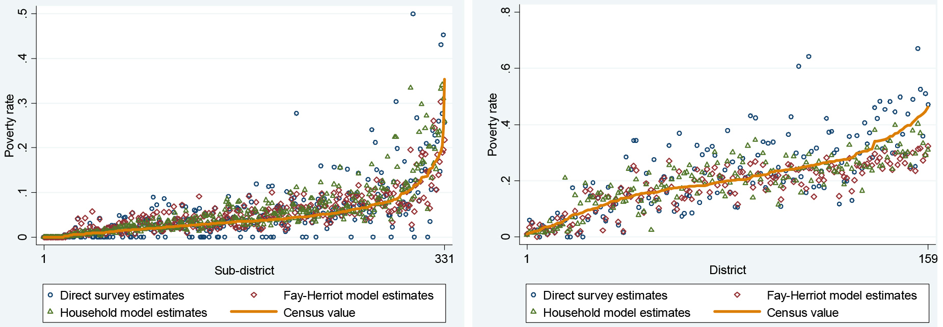
Figure 3.
Comparison of estimated Relative Mean Square Error by area and method for Sri Lanka (left) and Tanzania (right). Notes: Figures show mean squared errors of predicted asset-based poverty rates generated by household-level model, Fay-Herriot model, and Direct Survey estimates. Direct survey estimate MSEs top-coded at 0.015.
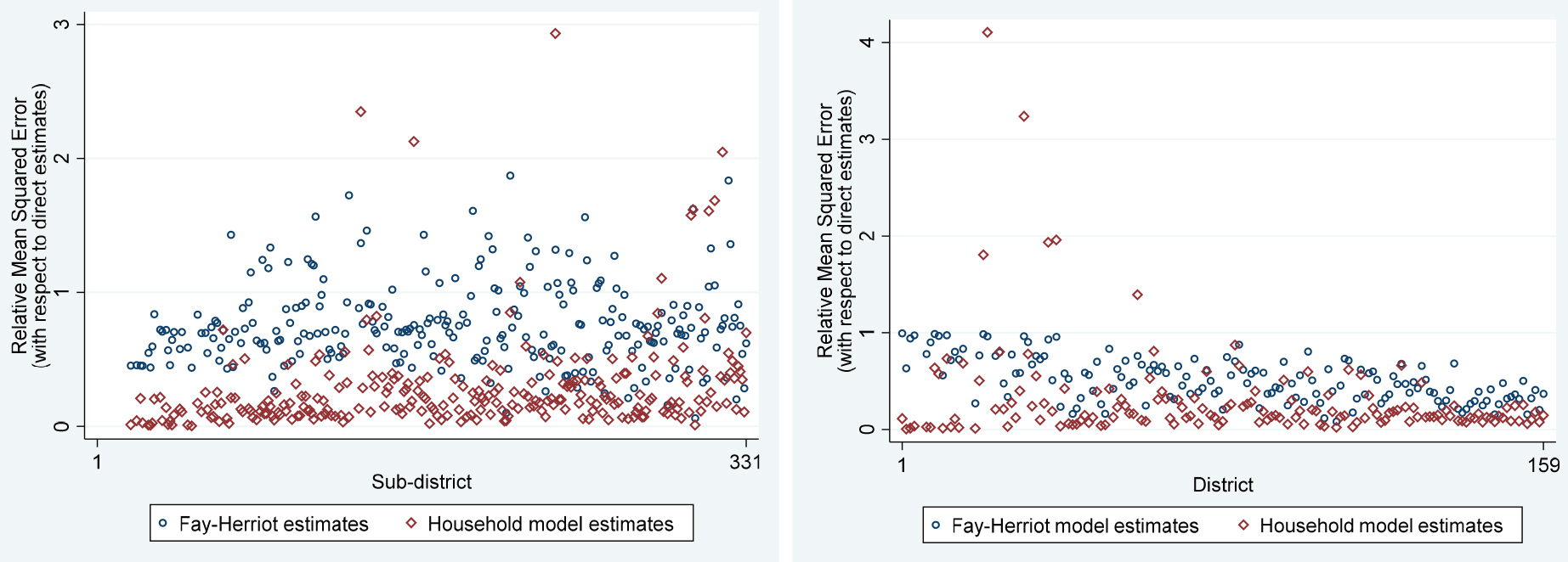
Figures 2 and 3 give a detailed look at the point estimates and mean squared errors for the area poverty estimates for each method. Sri Lanka is shown on the left panel and Tanzania on the right, and in each country the areas are ordered according to their non-monetary poverty rate in the census. The results clearly show that both Fay-Herriot and Household-level models greatly improve on the accuracy of the direct estimates, especially in areas with higher poverty rates. In Sri Lanka, many of the direct estimates are zero, even in high-poverty areas. The comparison between household models and Fay-Herriot models is less clear, but the Fay-Herriot estimates appear to be more prone to overestimate poverty for low-poverty areas and underestimate poverty for high-poverty areas.3737 Figure 3 presents the relative mean squared errors produced by the Fay-Herriot and Household model, relative to the direct estimates. It clearly demonstrates that the household model estimates are substantially more precise than both the Fay-Herriot estimates and the direct estimates for most target areas in both countries.
Table 5
Robustness check results for alternative methods for household level model
| Mean poverty | Mean MSE | Mean CV | RC | ARB | CR | |
|---|---|---|---|---|---|---|
| Sri Lanka | ||||||
| Baseline EB Estimates | 3.7 | 4.6 | 32.0 | 92.6 | 0.293 | 84.3 |
| Robustness check 1: No simulation weights | 3.7 | 4.8 | 31.9 | 92.6 | 0.294 | 82.8 |
| Robustness check 2: Box-Cox transformation | 3.5 | 4.7 | 31.2 | 92.8 | 0.296 | 81.9 |
| Robustness check 3: Stepwise ( | 3.7 | 4.7 | 27.9 | 92.1 | 0.292 | 80.7 |
| Robustness check 4: No Benchmarking | 3.7 | 4.2 | 39.1 | 90.2 | 0.212 | 82.2 |
| Robustness check 5: Use ELL instead of EBP | 3.7 | 17.5* | 62.4 | 90.6 | 0.321 | 99.1 |
| Tanzania | ||||||
| Baseline EB Estimates | 18.6 | 11.1 | 17.5 | 86.3 | 0.062 | 74.8 |
| Robustness check 1: No simulation weights | 18.3 | 11.8 | 17.8 | 85.5 | 0.060 | 73.0 |
| Robustness check 2: Box-Cox transformation | 15.8 | 13.1 | 18.7 | 85.8 | 0.051 | 76.1 |
| Robustness check 3: Stepwise ( | 18.8 | 9.8 | 16.4 | 84.6 | 0.060 | 69.8 |
| Robustness check 4: No Benchmarking | 18.6 | 9.7 | 17.5 | 82.6 | 0.012 | 69.8 |
| Robustness check 5: Use ELL instead of EBP | 19.8 | 55.9* | 38.0 | 84.6 | 0.043 | 95.6 |
Notes: Rows represent different variants of household-level model as listed in the table. Columns represent mean poverty rates, average mean squared error times 10,000, mean coefficient of variation, Spearman rank correlation with actual census value (RC), and coverage rate (CR). All means are unweighted across 331 subdistricts in Sri Lanka and 159 Districts in Tanzania. All results except for mean poverty reflect benchmarking to survey estimates for 25 districts in Sri Lanka and 25 regions in Tanzania. Asterisks (*) indicate mean estimated variance instead of mean squared error.
Finally, Table 4 compares the precision of the unit level model with the direct survey estimates for regions, which are districts in Sri Lanka and regions in Tanzania. The regions are levels for which the household survey is considered reliable and direct survey estimates of monetary poverty rates are published. In Sri Lanka, where there are 331 target areas, the mean squared errors for the subdistrict estimates are about sixty percent larger than the direct survey estimates for districts. In Tanzania, meanwhile, there are only 159 areas and the same number as regions as Sri Lanka. In this case, the average mean squared error of the small area district estimates is slightly lower than the direct estimates for regions, while the mean CV is modestly higher. This type of comparisons is useful to inform decisions by national statistics offices of whether small area estimates are sufficiently precise to publish.
5.Robustness checks for the household-level model
The previous section demonstrated that the house-hold-level model produced estimates that are substantially more efficient and as accurate as the area level model, while both the household level model and Fay-Herriot model both predicted poverty rates much more accurately than the direct estimates. The household-level model examined above was derived using a particular variant of the empirical best model, however, and it is informative to examine how the performance of the estimates varies based on different methodological choices.
The first robustness check relates to weighting the results of the household simulations by household size when aggregating across households, which is consistent with standard practice of calculating the poverty rate across individuals rather than households. The second robustness check considers using a Box-Cox transformation rather than an Ordered Quantile Normalization to transform the dependent variable in the model. This gives an indication of how much the use of the Ordered Quantile Normalization improves the results and ensures that the estimates remain reasonable when using a more traditional normalization method. The third robustness check considers the predictions when using a stepwise procedure, set with a probability threshold of 0.01, to select the model instead of the plugin lasso method. The fourth robustness check shows results when we do not benchmark the estimates to the survey estimates at the regional level. “The fifth robustness check” compares results from EBP versus ELL.
Table 6
Robustness check for noisy welfare measure
| Sri Lanka | Tanzania | |||||||||
|---|---|---|---|---|---|---|---|---|---|---|
| Mean poverty | Mean MSE | Mean CV | RC | CR | Mean poverty | Mean MSE | Mean CV | RC | CR | |
| Direct estimates (H-T approximation) | 4.0 | 15.9 | 65.3 | 58.0 | 74.6 | 20.0 | 82.3 | 45.4 | 80.1 | 83.0 |
| Area level Fay-Herriot model | 4.0 | 10.5 | 54.1 | 78.9 | 80.7 | 16.8 | 53.2 | 39.5 | 69.2 | 88.1 |
| Household-level EB model | 3.7 | 7.3 | 68.1 | 91.4 | 84.9 | 17.6 | 18.1 | 31.7 | 88.7 | 79.9 |
Table 7
Household-level diagnostics from the robustness check with noisy welfare measure
| Household model diagnostics | Sr Lanka | Tanzania | ||
|---|---|---|---|---|
| Marginal R | 0. | 196 | 0. | 208 |
| Conditional R | 0. | 304 | 0. | 329 |
| Skewness of area effect | 0. | 14 | 04 | |
| Kurtosis of area effect | 2. | 99 | 2. | 61 |
| Wilks-Shapiro P-value | 0. | 40 | 0. | 33 |
| Skewness of household error | 03 | 06 | ||
| Kurtosis of household error | 3. | 12 | 3. | 08 |
| Variance of estimated area effect | 0. | 110 | 0. | 122 |
| Variance of estimated household residual | 0. | 702 | 0. | 671 |
| Percentage of variance of error term due to area effect | 15. | 7% | 18. | 2% |
Table 5 displays the results of these robustness checks. For the purposes of brevity, we report the mean poverty, MSE, rank correlation, and coverage rate.3838 The estimator without simulation weights is slightly less accurate than those with weights in Sri Lanka and equally accurate in Tanzania, but is associated with a mild decline in both efficiency and coverage in both countries. The second robustness check uses a more standard Box-Cox transformation of the welfare variable instead of the ordered quantile normalization transformation. This leads to downward bias in the estimates in both countries, although the correlation and coverage rate changes little when using the Box-Cox transformation.3939 The models fit with stepwise regression, reported on the third row, are overfit in these two cases. This leads to less accurate predictions and lower coverage rates than the Lasso-selected model, especially in Tanzania. The fourth robustness check reports the results when the small area estimates are not benchmarked. Not benchmarking reduces mean MSE in both cases, although mean CV increases because estimated poverty rates for some small areas are closer to zero. In terms of accuracy, the non-benchmarked results remain highly correlated with the census in Sri Lanka. In Tanzania, the rank correlation falls from 86.3 to 82.6, and the coverage rate falls to 70 percent, indicating that benchmark moderately improved the accuracy of the estimates in Tanzania. Finally, the last row reports the results when an ELL method is used instead of the EBP method.4040 As measured by rank correlation, the ELL estimates are less accurate than EBP estimates in both countries.4141 In addition, ELL estimates are far less efficient than the EBP and FH estimates, because they do not condition on the household-level survey data. The mean variance estimates from ELL are approximately four to five times as large as the estimated MSEs in the baseline EBP estimates, with mean CVs that are only slightly below those of the direct estimates reported in Table 2. This leads to a coverage rate of about 99 percent in Sri Lanka, although the ELL coverage rate in Tanzania of about 96 percent is approximately correct.
The final robustness check examines how the baseline household level model fares when random noise is added to the welfare aggregate. This better approximates a monetary welfare measure such as per capita consumption or income, which contain a greater portion of unexplained variance resulting from both transient welfare shocks and measurement error. We add two error term components to the existing measure of non-monetary welfare. The first error component is an area effect, drawn form a normal distribution with mean zero and variance 0.5, and the second is a household specific error term with mean zero and variance 1. These variance values were chosen arbitrarily, with the aim of achieving a model
Table 6 displays the results when estimating area-level poverty using direct estimates, the Fay-Herriot model, and the household model with a noisier welfare aggregate, and Table 7 presents the key household model diagnostics from this robustness test. Overall, the results, with a few exceptions, are similar to the main results for the non-monetary welfare measure reported in Tables 2 and 3. The household level model produces the most precise estimates, as judged by the average estimated mean squared error across small areas. The average CV rises greatly in Sri Lanka, due to large positive outliers, when using the noisier measure. These outliers are areas with very low predicted poverty rates, yet high mean squared error, due to the greater variability in the area effect in these simulations. This illustrates that average CV should be interpreted with caution in settings with low poverty rates and highly variable area effects. Nonetheless, even with a noisier welfare aggregate, the reduction in mean squared error Sri Lanka compared with the direct estimates is approximately equivalent to doubling the size of the sample. In Tanzania, where the poverty rate is much higher, the household-level model leads to a 78 percent reduction in the mean squared error, a factor comparable to that reported in Table 3. The analogous reduction in average CV is 30 percent, which is also comparable to approximately doubling the sample size.
Turning to accuracy and coverage, exploiting village variation using the household model substantially improves accuracy, as measured by the rank correlation with the true noisier welfare measure. The rank correlation remains very high in Sri Lanka (0.91) and in Tanzania (0.87 percent) when using the noisier welfare measure. Finally, coverage rates for the household level model decline only modestly in Tanzania and increase significantly in Sri Lanka in comparison with the direct estimates. In Sri Lanka, the coverage rate reported in Table 6 for the noisy welfare measure is remarkably similar to the one for non-monetary poverty reported in Table 4 (84.9% vs. 83.7%). In Tanzania, the coverage rate is higher for the noisy welfare measure (78.0% vs. 73.6%). Accuracy and coverage are particularly important measures to consider because, unlike estimated precision, they are only observed when a “true” census population is available. Overall, the results presented in Table 6 indicate that the accuracy and coverage of the household level model remain high, in comparison with both the Fay-Herriot and direct estimates, when additional noise is introduced into the welfare measure.
6.Conclusion
This paper examines the extent to which combining a synthetic sample drawn from the census with geospatial data at the subarea level in Sri Lanka and Tanzania generates more precise and accurate estimates of non-monetary poverty. The analysis examines non-monetary poverty in order to evaluate the estimates against census data, which sheds light on the relative performance of different methodological approaches. The results are encouraging, and demonstrate that augmenting survey data with publicly available geospatial data substantially increases the accuracy and precision of small area estimates. The rank correlations between the small area estimates and the actual census are roughly 93 and 86 percent in Sri Lanka and Tanzania, respectively, which are significantly higher than the analogous correlations for the direct survey. The household-level model, compared with standard clustered survey estimates, reduces the mean squared error by about two-thirds in Sri Lanka and four-fifths in Tanzania, which is roughly equivalent to tripling and quintupling the effective sample size.
The financial cost of this type of small area estimation procedure is generally low and falling rapidly. Much of the auxiliary data used for the small area estimation, such as estimates of built-up area, nighttime lights, and vegetation, are freely available. There are two notable exceptions. First, the calculation of spatial features at a national scale requires constructing a cloud-free mosaic of Sentinel imagery, considerable computing power, and the expertise to implement software to calculate contextual features. Second, the data on Tanzanian building footprints are proprietary. However, data on building footprints are increasingly being released in the public domain and it is not difficult to envision information on building footprints becoming freely available for the entire world in the coming years, potentially through Open Street Map as it continues to improve in accuracy and coverage. Finally, access to subarea survey identifiers and shapefiles, or access to EA geocoordinates, is necessary to link survey data to geospatial indicators. This is not feasible in all contexts, but the growing popularity of geospatial analysis and CAPI data collection is making geospatial survey analysis more common. A conservative estimate is that the time and expertise required to generate these types of estimates costs $50,000 to $150,000. This is minor compared to the value created by even doubling the effective sample size of nationally representative household surveys that often cost at least a million dollars to field.
The results could be improved by further research and methodological development. One avenue for further research is to explore the performance of a subarea-level model, an extension of the Fay-Herriot model specified at the subarea level with an area-level mixed effect [42]. Estimating such a model at the subarea level makes it easier to properly account for sample design effects. However, modeling poverty rates as a linear function of predictors may generate less accurate estimates, especially when poverty rates are low. It would be useful to better understand how the results of a properly specified subarea model compare with a household-level model using subarea predictors. Secondly, further research could consider the issue of how to measure model performance in the absence of concurrent census data. The calculation of accuracy measures and coverage rates, in particular, requires a benchmark measure of truth. However, some model diagnostics presented in section 4 above, such as the estimated variance and distribution of the error terms, can be calculated from survey data. Benchmarking scale factors may also convey information about model bias at the regional level. However, further research is needed to better understand how best to assess the accuracy and reliability of small area estimates based on geospatial data in the absence of census data.
Notes
1 There is an extensive literature on updating small area estimates with new survey data using Structure-Preserving Estimation and variants, which assume that a subset of the coefficients remain constant over time [9, 10, 11].
2 A similar approach has been adopted in [12], which uses cluster-level characteristics derived from the census to generate small area estimates of poverty.
4 Tanzania throughout the paper refers to mainland Tanzania; Zanzibar is excluded from the analysis.
5 Villages are larger than the enumeration areas both in Sri Lanka and Tanzania. The boundary shapefiles for clusters or enumeration areas were not available for both countries.
6 The M-quantile method is not considered here because, like ELL, the predictions are purely synthetic and not conditioned on the sample, and therefore like ELL is less efficient than EBP when the model solely uses geographically aggregated predictors. Furthermore, unlike EBP and ELL, the M-quantile method has not yet to our knowledge been applied by a national statistics office to generate small area estimates.
7 Regions are defined as districts in Sri Lanka and regions in Tanzania. Our proposed approach of employing EBP with village-level characteristics to predict welfare does not necessarily yield regional estimates that are consistent with the direct survey estimates although it is important to align these two given that the household survey itself is representative at the regional level. To reconcile this discrepancy, we perform a benchmarking procedure [19, 20]. Below we also report results without benchmarking.
8 See the full details on a set of variables used in the principal component analysis in Appendix A.
9 These poverty rates are obtained from the 2018 Tanzania Household Budget Survey, and the 2016 Sri Lanka Household income and Expenditure Survey.
10 For each country, a one to one merge was carried out at the village level to identify which of the census villages appeared in the survey.
11 This indicator divides land into five main climate groups (tropical, dry, temperate, continental, and polar), with each group being divided based on seasonal precipitation and temperature patterns, based on a raster version of the map available at 0.5
12 See Appendix B for a full list of satellite and geospatial indicators used for the small area estimation of non-monetary poverty.
13 The following contextual features include: Fourier Transform (FT); Gabor Filter [27], Histogram of Oriented Gradients (HOG) [28]; Lacunarity (LAC) [29]; Line Support Regions (LSR) [30]; Normalized Difference Vegetation Index (NDVI); PanTex [31]; and lastly, Structural Feature Sets (SFS) [32]. Jordan Graesser’s Sp.Feas package was used to calculate these features.
14 For most features, we use scales of 3, 5, 7, which correspond to squares of 3 pixels by 3 pixels, 5 pixels by 5 pixels, and 7 pixels by 7 pixels.
15 The team also calculated spatial features using the Sp.Feas package for Tanzania based on Sentinel 2 imagery, but these were found to be highly colinear with the building footprint data and were therefore discarded.
16 Available at https://sites.research.google/open-buildings/.
17 The average population size of villages in Sri Lanka was 1,130 with the average land size of approximately 2 km
18 The average population size of villages in Tanzania was 2,178 with the average land size of approximately 20 km
19 This approximation is necessary because the variance of the H-T estimator depends on the joint inclusion probabilities of each pair of sample households, which is not known.
20 The survey contains no poor households in 5 of the 159 small areas in Tanzania and 111 of the 328 small areas in Sri Lanka.
21 See [45] for a comprehensive review of EBLUP models, and [46] for a comprehensive review of their application to small area estimation.
23 Sri Lanka is unique in that the national statistics office designates certain areas as the “Estate Sector”. The estate sector mainly consists of tea plantations and is historically economically disadvantaged.
24 See [47] which provides a thorough review on the issue of transformations for small area estimation in details. A log-shift transformation involves adding a constant to welfare prior to taking the log, while the Box-cox transformation can be written as:
25 To calculate small area estimates of the poverty gap, poverty severity, or inequality, it is critical to retransform the estimates back to the original welfare metric, as is done in the ELL method by exponentiating log welfare in each simulation. However, this retransformation is not necessary when estimating headcount poverty rates.
26 Practice can vary widely [47], for example, selects only 6 covariates present in Mexican census and survey data, based in part on the Akaike Information Criterion (AIC) from a standard OLS model. Most small area applications using ELL, however, use a considerably larger set of variables [49], for example, note that many successful applications include less than 20 household level variables. However, they also advocate including cluster-level means, which can boost the number of variables significantly past 20 or 30. Admittedly, the number of variables is an imperfect measure of model parsimony due to the potential inclusion of categorical variables.
27 We use the variant of the Stata plugin estimator that allows for heteroscedastic errors. The plugin method uses an iterative formula to select the lambda shrinkage parameter in the lasso instead of a grid search. The plug-in estimator tends to produce more parsimonious models than cross-validation, suggesting the models are underfit. See [50] and appendix A of [51] for technical details regarding the implementation of the plugin lasso estimator.
28 The scaling factor is defined as the ratio of the estimated poverty rate obtained from the survey to the population-weighted mean poverty rate of the small area estimates, for each region.
29 This leaves open the question of how to adjust the mean squared error estimates while benchmarking. Ideally, to obtain accurate estimates of the mean squared error, benchmarking would be performed by the small area estimation package within each bootstrap replication. Unfortunately, this option is not currently implemented in available software packages. As a second-best solution, we scale the mean squared error by the square of the same scaling factor that is applied to the point estimates, which leaves the coefficient of variation unchanged by the benchmarking process. Because the point estimates are slightly underestimated in Tanzania and Sri Lanka, this procedure increases the mean squared error and improves coverage rates.
30 The CV for each small area is defined as the ratio of the square root of the estimated mean squared error to the mean estimated poverty rate, a definition sometimes referred to as CV (RMSE). We report the average CV across areas.
31 The average relative bias equals the average, across areas of the ratio of the difference between the true and estimated poverty rates to the true poverty rate,
32 The Root Mean Square Error (RMSE) is equal to the square root for the average squared difference between the estimates and the actual census poverty rates.
33 See, for example, [52, 53, 54, 41] among many others. The upper and lower bounds of the confidence interval are determined by multiplying the square root of the estimated mean squared error by 1.96 and adding and subtracting it from the point estimate.
34 See Appendix C for more details on the model results.
35 These are village (sub-area) level regressions, and therefore the reported R2s do not apply to either to the unit-level household model nor the area-level model considered below.
36 [55] finds that the use of specific features identified in imagery, trained directly to a model predicting per capita consumption, rather than features derived from transfer learning increased predictive power by 31 percent in Uganda. This is consistent with the stronger performance seen in these models.
37 As described above, the Fay-Herriot estimates use the predicted poverty rate from the model in small areas where no sampled households are poor.
38 Results for all small areas are available upon request.
39 The sensitivity of the results to the choice of transformation is consistent with evidence from other studies, such as [47].
40 The random effect is specified at the target area level, to remain comparable with the EBP estimates.
41 Another difference between ELL and EBP is that the former estimates heteroscedasticity in the classical error term, which may help more in Tanzania than in Sri Lanka in this case.
Acknowledgments
This paper is a product of the Poverty and Equity global practice and a background report for the 2021 World Development Report. We are grateful to Nadia Belghith, Carlos Castelan, Robert Cull, Andrew Dabalen, Kristen Himelein, Dean Joliffe, Pierella Paci, Carolina Sanchez-Paramo, and Thomas Walker for their support. We thank Paul Corral, Kristen Himelein, Peter Lanjouw, and William Seitz for insightful comments and suggestions, and Partha Lahiri, Carl Morris and Roy van der Weide for helpful discussions. We also thank the anonymous reviewers for their careful reading of our manuscript and their many insightful comments and suggestions. Finally, we thank Albina Chuwa, Dilhanie Deepawansa, Keith Garrett, Amara Satharasinghe, and Elizabeth Talbert for their help in obtaining data. The findings, interpretations, and conclusions in this paper are entirely those of the authors. They do not necessarily represent the views of the World Bank Group, its Executive Directors, or the countries they represent.
Supplementary data
The supplementary files are available to download from http://dx.doi.org/10.3233/SJI-210902.
References
[1] | Yeh C, Perez A, Driscoll A, Azzari G, Tang Z, Lobell D, Ermon S, Burke M. Using publicly available satellite imagery and deep learning to understand economic well-being in Africa. Nature Communications. (2020) May 22; 11: (1): 1-1. |
[2] | Jean N, Burke M, Xie M, Davis WM, Lobell DB, Ermon S. Combining satellite imagery and machine learning to predict poverty. Science. (2016) Aug 19; 353: (6301): 790-4. |
[3] | Steele JE, Sundsøy PR, Pezzulo C, Alegana VA, Bird TJ, Blumenstock J, Bjelland J, Engø-Monsen K, De Montjoye YA, Iqbal AM, Hadiuzzaman KN. Mapping poverty using mobile phone and satellite data. Journal of The Royal Society Interface. (2017) Feb 28; 14: (127): 20160690. |
[4] | Engstrom R, Hersh JS, Newhouse DL. Poverty from space: using high-resolution satellite imagery for estimating economic well-being. World Bank Economic Review. (2022) May 36: (2): 382-412. |
[5] | Pokhriyal N, Jacques DC. Combining disparate data sources for improved poverty prediction and mapping. Proceedings of the National Academy of Sciences. (2017) Nov 14; 114: (46): E9783-92. |
[6] | Elbers C, Lanjouw JO, Lanjouw P. Micro-level estimation of poverty and inequality. Econometrica. (2003) Jan 1; 71: (1): 355-64. |
[7] | Tarozzi A, Deaton A. Using census and survey data to estimate poverty and inequality for small areas. The Review of Economics and Statistics. (2009) Nov 1; 91: (4): 773-92. |
[8] | Molina I, Rao JN. Small area estimation of poverty indicators. Canadian Journal of Statistics. (2010) Sep; 38: (3): 369-85. |
[9] | Purcell NJ, Kish L. Postcensal estimates for local areas (or domains). International Statistical Review/Revue Internationale de Statistique. (1980) Apr; 1: : 3-18. |
[10] | Isidro M, Haslett S, Jones G. Comparison of intercensal updating techniques for local level poverty statistics. In Proceedings of Statistics Canada Symposium (2010) ; pp. 10B-4. |
[11] | Isidro M, Haslett S, Jones G. Extended Structure Preserving Estimation (ESPREE) for updating small area estimates of poverty. The Annals of Applied Statistics. (2016) Mar; 10: (1): 451-76. |
[12] | Lange S, Pape UJ, Putz P. Small area estimation of poverty under structural change. World Bank Policy Research Working Paper. (2018) Jun; 12: (8472). |
[13] | Battese GE, Harter RM, Fuller WA. An error-components model for prediction of county crop areas using survey and satellite data. Journal of the American Statistical Association. (1988) Mar 1; 83: (401): 28-36. |
[14] | Datta GS, Day B, Maiti T. Multivariate Bayesian small area estimation: an application to survey and satellite data. Sankhyā The Indian Journal of Statistics, Series A. (1998) Oct 1: 344-62. |
[15] | Erciulescu AL, Cruze NB, Nandram B. Model-based county level crop estimates incorporating auxiliary sources of information. Journal of the Royal Statistical Society: Series A (Statistics in Society). (2019) Jan 1; 182: (1): 283-303. |
[16] | Chambers R, Tzavidis N. M-quantile models for small area estimation. Biometrika. (2006) Jun 1; 93: (2): 255-68. |
[17] | Das S, Haslett S. A comparison of methods for poverty estimation in developing countries. International Statistical Review. (2019) Aug; 87: (2): 368-92. |
[18] | Fay RE, Herriot RA. Estimates of income for small places: an application of James-Stein procedures to census data. Journal of the American Statistical Association. (1979) Jun 1; 74: (366a): 269-77. |
[19] | Pfeffermann D, Sikov A, Tiller R. Single-and two-stage cross-sectional and time series benchmarking procedures for small area estimation. Test. (2014) Dec; 23: (4): 631-66. |
[20] | Wang J, Fuller WA, Qu Y. Small area estimation under a restriction. Survey methodology. (2008) Jun 1; 34: (1): 29. |
[21] | Tzavidis N, Zhang L, Luna A, Schmid T, Rojas-Perilla N. From start to finish: a framework for the production of small area official statistics. Journal of the Royal Statistical Society: Series A (Statistics in Society). (2018) ; 181: (4): 927-979. |
[22] | Matsuura K, Willmott CJ. Terrestrial precipitation: 1900–2017 gridded monthly time series. Electronic. Department of Geography, University of Delaware, Newark, DE. (2018) ; 19716. |
[23] | CGIAR-CSI SR. 90m Digital Elevation Database v4. 1, unpublished data. |
[24] | Hansen MC, Potapov PV, Moore R, Hancher M, Turubanova SA, Tyukavina A, Thau D, Stehman SV, Goetz SJ, Loveland TR, Kommareddy A. High-resolution global maps of 21st-century forest cover change. Science. (2013) Nov 15; 342: (6160): 850-3. |
[25] | Kottek M, Grieser J, Beck C, Rudolf B, Rubel F. World map of the Köppen-Geiger climate classification updated. |
[26] | Koo J, Cox CM, Bacou M, Azzarri C, Guo Z, Wood-Sichra U, Gong Q, You L. CELL5M: A geospatial database of agricultural indicators for Africa South of the Sahara. F1000 Research. (2016) ; 5: . |
[27] | Mehrotra R, Namuduri KR, Ranganathan N. Gabor filter-based edge detection. Pattern recognition. (1992) Dec 1; 25: (12): 1479-94. |
[28] | Dalal N, Triggs B. Histograms of oriented gradients for human detection. In 2005 IEEE computer society conference on computer vision and pattern recognition (CVPR’05) 2005 Jun 20 (Vol. 1, pp. 886-893). IEEE. |
[29] | Myint SW, Mesev V, Lam N. Urban textural analysis from remote sensor data: Lacunarity measurements based on the differential box counting method. Geographical Analysis. (2006) Oct; 38: (4): 371-90. |
[30] | Unsalan C, Boyer KL. Classifying land development in high-resolution panchromatic satellite images using straight-line statistics. IEEE Transactions on Geoscience and Remote Sensing. (2004) Apr 19; 42: (4): 907-19. |
[31] | Pesaresi M, Gerhardinger A, Kayitakire F. A robust built-up area presence index by anisotropic rotation-invariant textural measure. IEEE Journal of Selected Topics in Applied Earth Observations and Remote Sensing. (2008) Oct 28;1: (3): 180-92. |
[32] | Huang X, Liangpei Z, Li P. Classification and extraction of spatial features in urban areas using high-resolution multispectral imagery. IEEE Geoscience and Remote Sensing Letters. (2007) ; 4: (2): 260-264. |
[33] | Engstrom R, Newhouse D, Soundararajan V. Estimating small-area population density in Sri Lanka using surveys and Geo-spatial data. PloS One. (2020) Aug 5; 15: (8): e0237063. |
[34] | Chao S, Engstrom R, Mann M, Bedada A. Evaluating the Ability to Use Contextual Features Derived from Multi-Scale Satellite Imagery to Map Spatial Patterns of Urban Attributes and Population Distributions. Remote Sensing. (2021) Jan; 13: (19): 3962. |
[35] | Huber PJ. Under Nonstandard Conditions. In Proceedings of the Fifth Berkeley Symposium on Mathematical Statistics and Probability: Weather modification, (1967) (Vol. 5, p. 221). Univ of California Press. |
[36] | Rogers W. Regression standard errors in clustered samples. Stata Technical Bulletin. (1994) ; 3: (13). |
[37] | Horvitz DG, Thompson DJ. A generalization of sampling without replacement from a finite universe. Journal of the American statistical Association. (1952) Dec 1; 47: (260): 663-85. |
[38] | Stein C, James W. Estimation with quadratic loss. In Proc. 4th Berkeley Symp. Mathematical Statistics Probability. (1961) ; 1: : 361-379. |
[39] | Halbmeier C, Kreutzmann AK, Schmid T, Schröder C. The fayherriot command for estimating small-area indicators. The Stata Journal. (2019) Sep; 19: (3): 626-44. |
[40] | Haslett S. Small Area Estimation Using Both Survey and Census Unit Record Data: Links, Alternatives, and the Central Roles of Regression and Contextual Variables, in Monica Pratesi (ed)., Analysis of Poverty Data by Small Area Estimation, John Wiley and Sons Ltd, West Sussex, United Kingdom, (2016) , pp. 327-348. |
[41] | Elbers C, Lanjouw P, Leite PG. Brazil within Brazil: Testing the Poverty Map Methodology in Minas Gerais. Policy Research Working Paper, (2008) ; No. 4513. World Bank, Washington, DC. © World Bank. https://openknowledge.worldbank.org/handle/10986/6575 License: CC BY 3.0 IGO. |
[42] | Torabi M, Rao J. On small area estimation under a sub-area level model. Journal of Multivariate Analysis. (2014) May 1; 127: : 36-55. |
[43] | Corral RP, Seitz W, Azevedo JP, Nguyen MC. FHSAE: Stata module to fit an area level Fay-Herriot model, (2018) . |
[44] | Chandra H, Sud UC, Gupta VK. Small area estimation under area level model using R software. New Delhi: Indian Agricultural Statistics Research Institute, (2013) . |
[45] | Morris CN. Parametric empirical Bayes inference: theory and applications. Journal of the American statistical Association. (1983) Mar 1; 78: (381): 47-55. |
[46] | Jiang J, Lahiri P. Mixed model prediction and small area estimation. Test. (2006) Jun; 15: (1): 1-96. |
[47] | Tzavidis N, Zhang LC, Luna HA, Schmid T, Rojas-Perilla N. From start to finish: a framework for the production of small area official statistics. Journal of the Royal Statistical Society: Series A (Statistics in Society). (2018) ; 181: (4): 927-79. |
[48] | Peterson RA, Cavanaugh JE. Ordered quantile normalization: a semiparametric transformation built for the cross-validation era. Journal of Applied Statistics. (2019) Jun 15. |
[49] | Zhao Q, Lanjoouw P. User manual for povmap. World Bank. http://siteresources.worldbank.org/INTPGI/Resources/342674-1092157888460/Zhao_ManualPovMap.pdf. (2006) . |
[50] | Belloni A, Chernozhukov V. High dimensional sparse econometric models: An introduction. InInverse Problems and High-Dimensional Estimation, Springer, Berlin, Heidelberg, (2011) , pp. 121-156. |
[51] | Belloni A, Chernozhukov V, Hansen C. Inference on treatment effects after selection among high-dimensional controls. The Review of Economic Studies. (2014) Apr 1; 81: (2): 608-50. |
[52] | Tarozzi A. Can census data alone signal heterogeneity in the estimation of poverty maps. Journal of Development Economics. (2011) Jul 1; 95: (2): 170-85. |
[53] | Pratesi M, Salvati N. Small area estimation: the EBLUP estimator based on spatially correlated random area effects. Statistical Methods and Applications. (2008) Feb 1; 17: (1): 113-41. |
[54] | Hidiroglou MA, You Y. Comparison of unit level and area level small area estimators. Survey Methodology. (2016) Jun 1; 42: (1): 41-61. |
[55] | Ayush K, Uzkent B, Burke M, Lobell D, Ermon S. Generating interpretable poverty maps using object detection in satellite images. arXiv preprint arXiv:2002.01612. 2020 Feb 5. |
[56] | Engstrom R, Pavelesku D, Tanaka T, Wambile A. Mapping poverty and slums using multiple methodologies in Accra, Ghana. In 2019 Joint Urban Remote Sensing Event (JURSE), (2019) May 22; pp. 1-4. IEEE. |
[57] | Engstrom R, Harrison R, Mann M, Fletcher A. Evaluating the Relationship Between Contextual Features Derived from Very High Spatial Resolution Imagery and Urban Attributes: A Case Study in Sri Lanka. In 2019 Joint Urban Remote Sensing Event (JURSE), (2019) May 22; pp. 1-4. IEEE. |
[58] | Sandborn A, Engstrom RN. Determining the relationship between census data and spatial features derived from high-resolution imagery in Accra, Ghana. IEEE Journal of Selected Topics in Applied Earth Observations and Remote Sensing. (2016) Feb 11; 9: (5): 1970-7. |
[59] | World Bank. Tanzania mainland poverty assessment. World Bank; (2019) Dec 8. |


