Estimating excess mortality in Canada during the COVID-19 pandemic: Statistical methods adapted for rapid response in an evolving crisis

Sirag, Elham; Gissler, Gautier

doi:10.3233/SJI-210871

Estimating excess mortality in Canada during the COVID-19 pandemic: Statistical methods adapted for rapid response in an evolving crisis

Article type: Research Article

Authors: Sirag, Elham^{a; *} | Gissler, Gautier^b

Affiliations: [a] Centre for Demography, Statistics Canada, Ottawa, ON, Canada | [b] Statistical Integration Methods Division, Statistics Canada, Ottawa, ON, Canada

Correspondence: [*] Corresponding author: Elham Sirag, Centre for Demography, Statistics Canada, 100 Tunney’s Pasture Driveway, Ottawa, K1A 0T6, Canada. Tel.: +1 343 548 1460; E-mail: [email protected].

Keywords: Statistics Canada, excess mortality, Farrington algorithm, undercoverage, COVID-19

DOI: 10.3233/SJI-210871

Journal: Statistical Journal of the IAOS, vol. 37, no. 4, pp. 1173-1180, 2021

Published: 26 November 2021

Get PDF

Abstract

This paper presents the approach adopted at Statistics Canada to produce timely and accurate estimates of excess mortality during the ongoing COVID-19 pandemic. It focuses primarily on the two models involved in the estimation of excess mortality: the model used to estimate the expected number of deaths in the absence of the pandemic (baseline mortality), and the model used to adjust provisional death counts for undercoverage. We describe both, including how the models were adapted to fit our specific criteria as well as the various limitations they both possess. We conclude by presenting selected results from Statistics Canada’s official release of excess mortality estimates from February 8th, 2021.

1.Introduction

In the face of the ongoing pandemic, it is crucial for national governments to obtain precise measures of the impact of COVID-19 on the health outcomes of their populations. In Canada, while the tracking of vital statistics is the responsibility of provincial and territorial governments, Statistics Canada is the federal agency tasked with all official dissemination of these data. As a response to the pandemic, Statistics Canada has begun producing estimates of excess mortality1 1 as one means of quantifying COVID-19’s effect on mortality in Canada. Defined as the number of all-cause deaths observed during a crisis above and beyond what would be expected under “normal circumstances” [1], excess mortality provides a means of measuring the full impact of the pandemic by incorporating both direct effects – i.e. deaths caused by COVID-19 – as well as indirect effects, such as deaths with COVID-19 as a contributing cause, or deaths caused by circumstances surrounding the pandemic.

Many challenges surround the estimation of excess mortality within Canada. Unlike others countries2 2 that had developed surveillance systems to monitor abnormalities in weekly death counts prior to the pandemic, Statistics Canada had no such network in place. Moreover, death data provided to Statistics Canada by regional offices are often subject to significant delays, impacting our ability to disseminate death estimates in a timely fashion. Long reporting delays also inhibit us from adopting existing models for excess mortality if complete coverage of death data is an underlying assumption.

This paper describes the authors’ contributions to tackling these defined challenges in order to develop a method that would allow for the monthly production of excess mortality estimates at Statistics Canada. Section 2 describes the model used to estimate baseline (expected) mortality, and Section 3 the method used to adjust provisional death counts for reporting delays. Section 4 describes the method used to produce excess mortality estimates, along with 95% confidence intervals, and presents selected results from one of Statistics Canada’s recent releases. The final section presents our conclusion.

2.Estimating baseline mortality

Baseline mortality – defined as the number of deaths that would be expected to occur within the population of interest in the absence of the COVID-19 pandemic – is the first of two components required in the computation of excess mortality. Numerous challenges surround the accurate estimation of baseline mortality, each of which impacted our selection of a method.

The largest challenge concerns the selection of a reference period. Deaths counts in Canada are frequently subject to large relative year-to-year fluctuations due to death being a statistically rare event. Moreover, changes in yearly observed death counts may reflect changes in the composition of a population – such as an evolving population age structure, for example – in addition to true changes in mortality outcomes. The selection of a reference period thus requires a balance between being long enough to capture underlying trends in the presence of large annual variance, and being short enough to ensure that large changes in the population composition over time do not result in over- or under-estimation of expected deaths.

Other challenges in estimating baseline mortality involve modelling seasonality in the death data and ensuring that periods of historically high death counts in the reference period do not result in overestimation of baseline mortality. The selection of a model was made taking these challenges into consideration.

2.1Model

The model used to compute the expected number of deaths is based on an infectious disease surveillance algorithm for Poisson count data developed by Farrington et al. [2]. The same model is used in the Centre for Disease Control’s (CDC) own computation of excess deaths in the United States [3].

The model is implemented in R with the use of the Surveillance package [4]. The method is described as follows. An overdispersed Poisson GLM with linear time trend and seasonal adjustment factors is fit to all-cause weekly death based on a rolling reference period spanning 2016 to 2020.3 3 Models are fit for the total population and for the population disaggregated by age group (0–44, 45–64, 65–84, and 85+), sex, and age & sex group for each of the provinces and territories.4 4 Historical death counts used to the fit the model are a combination of published death data from the Canadian Vital Statistics Death Database (2016–2019)5 5 and provisional death counts from the National Routing System (2019).6 6

Mathematically, the model can be expressed using the following log-linear configuration:

log⁡μt=α+β⁢t+γc⁢(t)

where:

• μt is defined as the expected death count in week t
• α is the model intercept
• β is the coefficient corresponding to the linear time trend in week t
• γc⁢(t) is the seasonal factor level corresponding to week t

Seasonality is modelled by dividing the fifty-two weeks of the year into ten distinct periods – one seven-week period corresponding to the current week t± three weeks, and nine five-week periods for the rest of the year. A factor variable equivalent to a zero-order spline with eleven knots is then incorporated into the regression model.

Noufaily et al. [7] propose certain adjustments to the original Farrington algorithm in order to minimize the effect of historical periods of increased mortality on estimates of expected deaths, and to prevent periods of increased mortality leading up to the week being estimated, i.e. an ongoing outbreak, from impacting estimates. In the case of the former, once a model is fit to the data, residuals7 7 for each estimate in the reference period are computed. Any week with its residual, st, larger than 2.58 is down weighted in the following manner:

wt={γ⁢st-2if ⁢st>2.58γotherwise

where wt is the weight corresponding to week t, and γ is a weight normalizing constant. The model is then re-fit using the newly computed weights, and expected counts are re-estimated.

With regard to accounting for ongoing outbreaks, they suggest omitting the twenty-six weeks preceding the current week, t, from estimation, so that if a disease outbreak has begun in the weeks preceding week t, the expected count in that week will not be overestimated as a result.

95% confidence intervals8 8 are then computed for the estimates by assuming that the death count in week t follows a negative binomial distribution with mean μ^t and size parameter μ^t/(ϕ^t-1), where μ^t is the expected count and ϕ^t is the estimated overdispersion parameter in week t, defined:9 9

ϕ^t=max

{1(t-26)-p⁢∑m=t-xt-26wm⁢(ym-μ^m)2μ^m,1}

Where x refers to the total number of historical weeks preceding week t included in the reference period, and p the number of parameters in the model.

As of August 2020, this model has been used to produce estimates of expected deaths monthly for every week10 10 of 2020 beginning with the week ending January 4th and up until a predetermined cut-off date.11 11

2.2Limitations

This model possesses three primary limitations. First, the method used to compute confidence bounds, developed by Noufaily et al. [7], incorporates neither parameter uncertainty nor estimation uncertainty. Using the estimated μ^t and ϕ^t as the parameters of the negative binomial distribution corresponding to the predicted count in week t, y^t, and using its quantiles to obtain a prediction interval is equivalent to treating the estimated parameters as known. Salmon et al. [4] developed an alternative method that tries to partially correct this. They use the asymptotic Normality of μ^t to derive an upper 100⁢(1-α) quantile for its estimate, and incorporate this into the computation of the bounds. We tested both methods in the computation of upper and lower bounds, and found little difference between the two, however.

The second limitation is more a consequence of reporting delays present in the provisional death data. Since only the twenty-six weeks preceding each week are omitted from the reference period, 2020 death data are used in the estimation of counts for every week after the week of July 4th (the 27th week of the year). However, 2020 death data are considered preliminary and must be adjusted for reporting delays.12 12 Using unadjusted death counts as inputs in the computation of expected deaths may lead to underestimation of expected counts. Moreover, a consequence of the ongoing pandemic is elevated death counts over the course of the entire year. Including 2020 data in the reference period may result in underestimation of excess mortality when producing estimates post-pandemic. To correct for this, we designated the week of March 28th, 2020 as a cut-off week13 13 so that estimation for any week that included data past this date would have its reference period truncated accordingly. The result is that models fit to data in more recent weeks (week forty onwards) will have an increasingly dated reference period in comparison to older weeks.

A final limitation is the lack of an available means to evaluate the model’s overall performance. The algorithm is intended to detect aberrancies in count data, implying that fitting the model to an alternative reference period or assessing the model’s accuracy in estimating historical counts is of little value. Weeks with historical death counts above expected values may be due to external factors (such as a particularly severe flu season) and is thus not necessarily indicative of poor model performance. Regardless, the models were used to estimate counts in historical years (2018–2019), and it was found that they did reasonably well at predicting the overall trend in death counts. Results were also validated by comparing the sums of the disaggregated models to the models fit to the total counts.

3.Adjusting provisional death counts

The period of time between the date of a death and the date the death is received by Statistics Canada is referred to as the delay. In some provinces and territories, recent death data may not be complete – i.e. all of the deaths have not yet been received – until months after the date of death. Exceptional circumstances brought on by the COVID-19 pandemic may also put additional strain on local health care systems, leading to further delays. Our selection of a model was thus motivated by the need for a method that could handle delays of widely varying length that may change rapidly over time.

3.1Model

The method we adopt is a nowcasting approach that adjusts for incompleteness by evaluating the distribution of reporting delays observed within a set period of time, defined [t0;tmax]. This date of the period end, tmax, is extended with every subsequent release of Statistics Canada’s excess mortality estimates, and the key assumption is that the number of deaths occurring at the start of the period, t0 (the first week), are considered complete. Since death reporting processes in Canada have changed over time – and consequently the distribution of historical delays – we include only data from 2020 in the reference period.

To evaluate the distribution of delays (measured in weeks), observed deaths, denoted Yt,d, are indexed by their date of occurrence, t, and their date of reception, t+d, with t0⩽t⩽tmax. Consequently, for deaths occurring on date t, only delays, d, smaller than tmax-t can be observed.

Yt,d is modeled using a Poisson regression method developed by Brookmeyer and Damiano [8] and adapted by Seaman and De Angelis [9],14 14 defined:

Log⁢(E⁢(Yt,d))=αt+βd

For a death occurring within the reference period, the estimated probability that the reporting delay equals d weeks, given that it is less than or equal to d weeks is:

g^d=exp⁡{β^d}∑k=0dexp⁡{β^k}

Thus, the estimated probability that, for a death occurring during the reference period and received within m weeks, the reporting delay is less than or equal to d weeks is given by:

P(D⩽d|D⩽m)=∏j=d+1m(1-g^j)

The adjusted number of deaths occurring in week t is then computed by dividing the observed death count by the estimated probability that the reporting delay is less than or equal to dmax-(t-t0) weeks, where dmax=tmax-t0 is the maximum observable delay.

Adjusted number of deaths ⁢(t)

=∑d=0dmax-tYt⁢dP(D⩽dmax-(t-t0)|D⩽dmax)

3.2Limitations

The described approach does possess some limitations. The first relates to the assumption of a completion rate of 100% at t=t0. Since this may not hold true, we experimented with varying t0 slightly, and found that it did not significantly impact the results. We also found that with each successive release, very few deaths were retroactively added to the first week t0.

Moreover, the model assumes there is no change in the reception rate within the reference period. However, experiments using alternative reference periods did show changes in the distribution of reporting delay for certain provinces in 2020, likely attributable to the pandemic. To account for this, the reference period was divided into two based on observed shifts in reporting delays: the pre-pandemic period, beginning the first week of 2020, and the pandemic period, beginning on the 12th week of 2020 (from here on denoted t𝑝𝑎𝑛𝑑𝑒𝑚𝑖𝑐). This second period coincides with when the COVID-19 pandemic was beginning to have an impact in Canada. Figure 1 displays the adjustments resulting from these two periods for Canada as an example. Using only the first period to compute the distribution of reporting delays may lead to inaccurate predictions, especially for deaths observed later in the year during the height of the pandemic. Consequently, the second period was judged more relevant to illustrate recent trends than the first.

Figure 1.

Observed death counts and adjusted estimates for Canada, January 2020 to September 2020. Source: Statistics Canada’s monthly release on excess deaths. Available here: https://www150.statcan.gc.ca/n1/daily-quotidien/201028/dq201028b-eng.htm.

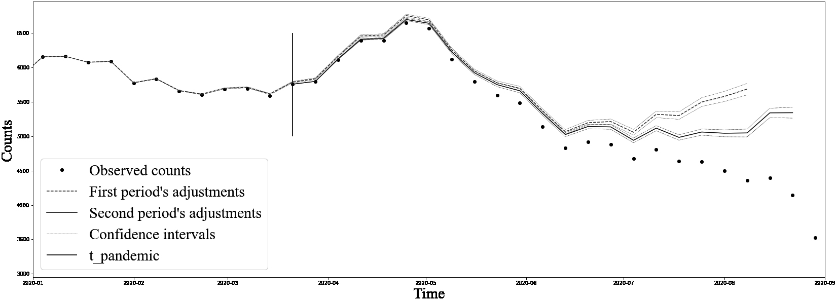
To minimize the impact of changes in the rate of reception, we use results obtained from the pre-pandemic period, t0 to t𝑝𝑎𝑛𝑑𝑒𝑚𝑖𝑐, in combination with results from the pandemic period, t𝑝𝑎𝑛𝑑𝑒𝑚𝑖𝑐 to tmax. Adding a third reference period was considered, but tests showed no further significant changes in the distribution of delays after the start of the second period. Without correction, the use of both periods results in a discontinuity at t𝑝𝑎𝑛𝑑𝑒𝑚𝑖𝑐 since it is used as the start of the second period (i.e. no undercoverage), but not the start of the first (undercoverage):

∑d=0dmax-t𝑝𝑎𝑛𝑑𝑒𝑚𝑖𝑐Yt𝑝𝑎𝑛𝑑𝑒𝑚𝑖𝑐,dPpre-pandemic(D⩽dmax-(t𝑝𝑎𝑛𝑑𝑒𝑚𝑖𝑐-t0)|D⩽dmax)

>∑d=0dmax-t𝑝𝑎𝑛𝑑𝑒𝑚𝑖𝑐Yt𝑝𝑎𝑛𝑑𝑒𝑚𝑖𝑐,d

Adjusted number of deathspre-pandemic⁢(t𝑝𝑎𝑛𝑑𝑒𝑚𝑖𝑐-)

>Adjusted number of deaths𝑝𝑎𝑛𝑑𝑒𝑚𝑖𝑐⁢(t𝑝𝑎𝑛𝑑𝑒𝑚𝑖𝑐+)

To ensure continuity, adjusted counts for deaths occurring during the pandemic period are increased by a multiplicative factor α, defined:

α=[Ppre-pandemic(D⩽dmax-(t𝑝𝑎𝑛𝑑𝑒𝑚𝑖𝑐-t0)|

D⩽dmax)]-1

Thus:

Adjusted counts ⁢(t)

={Adjusted number of deathspre-pandemic⁢(t)if ⁢t⩽t𝑝𝑎𝑛𝑑𝑒𝑚𝑖𝑐α×Adjusted number of deaths𝑝𝑎𝑛𝑑𝑒𝑚𝑖𝑐⁢(t)𝑒𝑙𝑠𝑒

One final issue relates to the quality of adjustments for deaths occurring at the very end of the reference period. A large degree of adjustment implies that very few observed deaths are available, and the model is thus more sensitive to variations in observed counts. We thus impose a minimum coverage threshold, Q, that estimates must satisfy. Final estimates of adjusted counts are released only for weeks where the coverage rates satisfy this threshold.

∀t∈[t0;tmax], if

P(D⩽dmax-(t-t0)|D⩽dmax)⩾Q,

Final adjusted counts ⁢(t)=Adjusted counts ⁢(t)

For all of Statistics Canada’s releases between August 2020 and February 2021, a threshold of Q= 75% was selected, offering a sufficient balance between accuracy and timeliness of outputs.

Based on this methodology, adjusted death counts were produced for each of the provinces and territories. Validation of the adjustments disaggregated by age group, sex, and age group and sex was done by ensuring that they were similar to those obtained from regional aggregate models. The relevance of the adjustments can be validated a posteriori with future releases, as shown in Fig. 3. Figure 2 displays final adjusted counts produced at the Canada-level from Statistics Canada’s October 2020 release. A divergence in trends between adjustments resulting from the two different periods can be observed, signifying substantial change in the distribution of delays.

Figure 2.

Comparison of adjusted death counts from the first and second periods, Canada, January 2020 to September 2020. Source: Statistics Canada’s monthly release on excess deaths. Available here: https://www150.statcan.gc.ca/n1/daily-quotidien/201028/dq201028b-eng.htm.

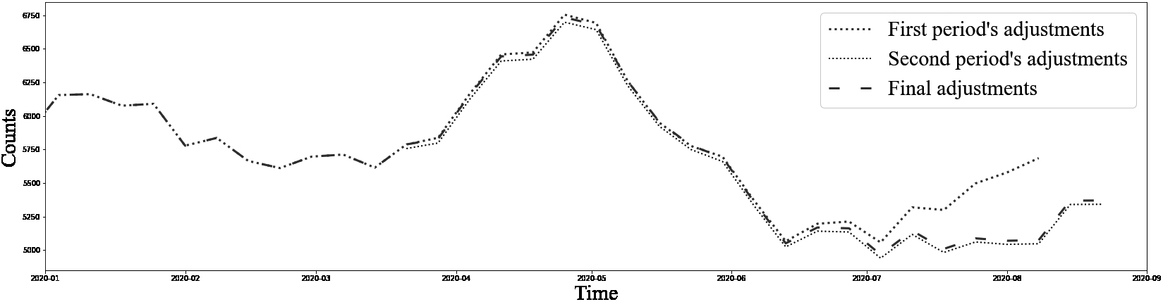
Figure 3.

Comparison of estimated adjustments for Canada based on Statistics Canada’s October 28th, 2020 release and February 8th, 2021 release. Source: Statistics Canada’s monthly releases on excess deaths. Available here: https://www150.statcan.gc.ca/n1/daily-quotidien/201028/ dq201028b-eng.htm.

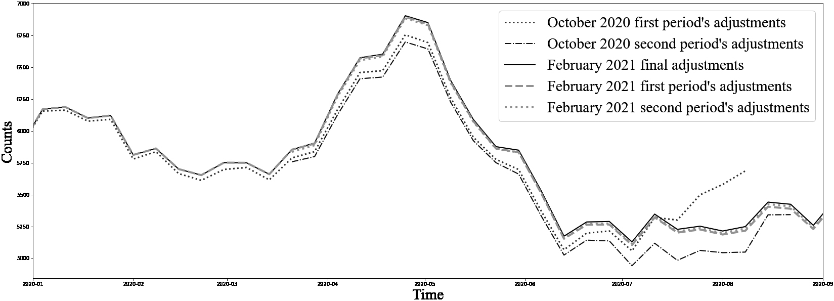
A posteriori validation demonstrated that adjustments are generally slightly underestimated, partially because the true distribution of the delays over the course of the entire pandemic is unknown and constantly evolving. As shown in Fig. 3, the difference in the distribution of delays over time provides justification for the use of a second reference period, which has a higher capacity to capture recent trends than the first period.

4.Excess mortality

Excess deaths for a given week are computed simply as the difference between the adjusted observed count and the expected count. In order to compute an estimate of variance, an assumption about the dependence between the processes used to generate adjusted and expected death counts must be made. We choose to assume independence between the two in order to simplify computations. While it may be possible that the distribution of reporting delays is correlated with the number of expected deaths, obtaining an accurate estimate of correlation is made difficult by a number of factors. One issue is that expected deaths are estimated based on a historical reference period of four years, while the distribution of reporting delays is based on only a 2020 reference period. Defining the covariance between the two processes when only one of them (i.e. expected deaths) accounts for annual seasonal patterns would likely lead to a misrepresentation of the true relationship.

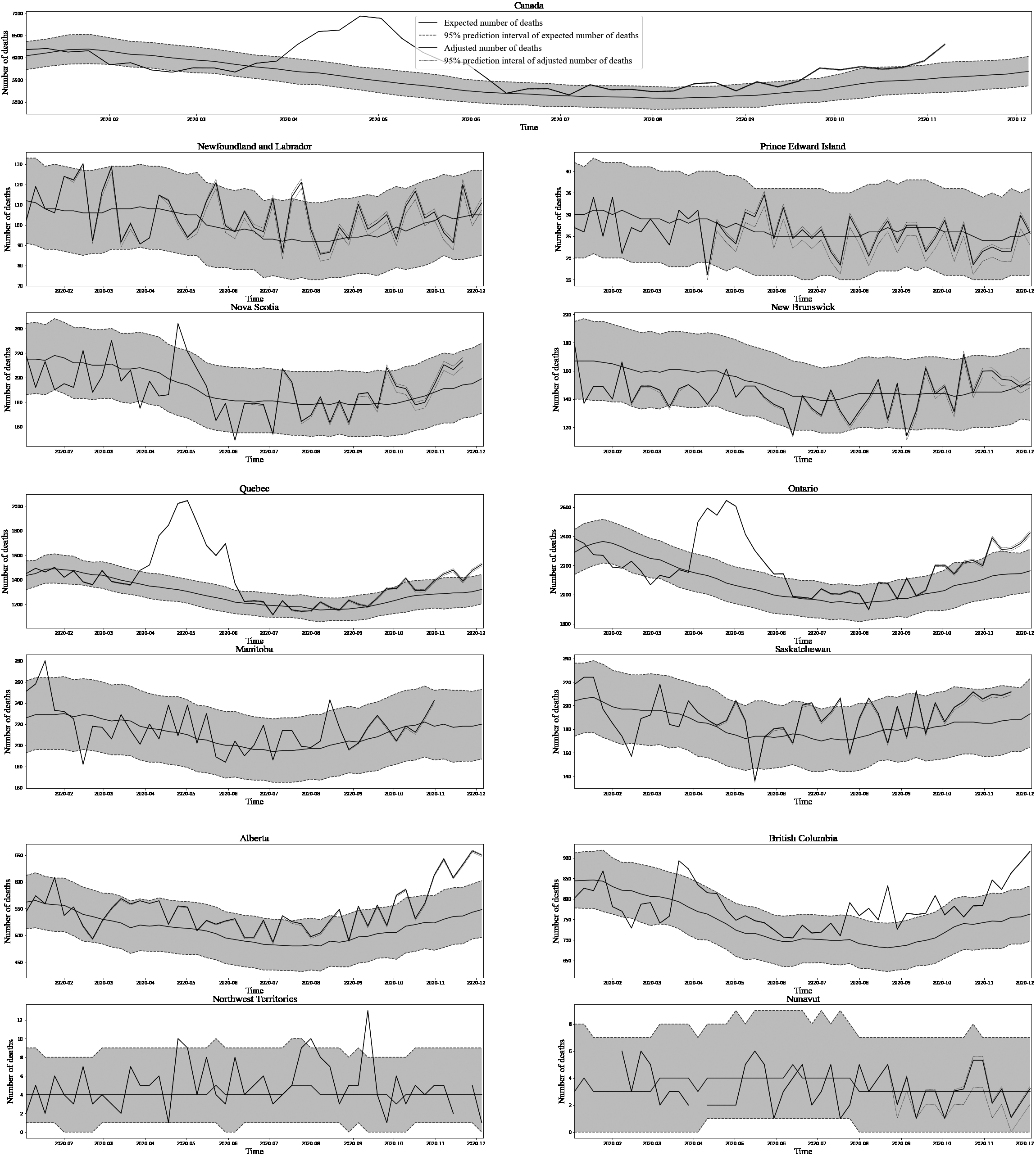
Figure 4.

Aggregate excess mortality estimates from Statistics Canada’s February 8th, 2021 release. Source: Statistics Canada’s monthly releases on excess deaths. Available here: https://www150.statcan.gc.ca/n1/daily-quotidien/201028/dq201028b-eng.htm.

To estimate variance, one possibility we considered was to use the Normal approximation to the distribution of expected counts (negative binomial) and to the distribution of adjusted counts (Poisson), so that the resulting distribution of excess deaths would be Normal. While this approximation was fairly accurate when it came to the distribution of expected counts on the provincial aggregate level, it became increasingly worse the further counts were disaggregated. Given this finding, we decided to adopt an empirical approach that made minimal additional assumptions. The method is described as follows.

1) 10,000 bootstrap samples15 15 of adjusted counts for each week in 2020 were generated for each of the models;
2) 10,000 samples16 16 from the distribution of expected counts were generated for each of the corresponding weeks and for each model;
3) Each of the 10,000 samples of adjusted counts was paired with the 10,000 samples of expected counts in the sampling order (i.e. they were not paired randomly), and 10,000 estimates of excess mortality were obtained by subtracting the two;
4) A 95% confidence interval was obtained by taking the 0.025 and 0.0975 quantiles of the empirical distribution of these excess mortality estimates.

Figure 4 below displays aggregate estimates of excess deaths along with corresponding 95% confidence intervals for each of the provinces and territories from Statistics Canada’s release covering deaths from the period January 1st, 2020 to December 5th, 2020.

5.Conclusion

The statistical methods presented in this paper were intended to help minimize estimation uncertainty arising from incompleteness in reported death counts and in baseline mortality in order to produce timely and accurate estimates of excess mortality. The estimates produced by our methods have been widely used externally as a means of both measuring the impact of COVID-19 in Canada and as a means of placing the situation in Canada within a global context. It is the authors’ goal to improve our current methods by adapting them as the pandemic evolves, and by developing long-term solutions to the limitations outlined in this

paper. We hope that our contribution will eventually lead to the implementation of an up-to-date mortality surveillance system in Canada.

Notes

1 Excess deaths and excess mortality are used interchangeably throughout this paper.

2 Such as those participating in the European Mortality Monitoring Project (EuroMOMO). See: euromomo.eu.

3 A four year reference period was selected after conducting various tests with periods of alternating length.

4 There are certain exceptions. Too few death counts resulted in unreliable disaggregated estimates in Prince Edward Island, Nunavut, and the Northwest Territories. Only totals were released for these regions. No estimates were produced for Yukon, due to lack of available data.

5 The Canadian Vital Statistics Death Database is an administrative database that collects monthly and annual information on deaths from the provincial and territorial vital statistical offices in Canada [5].

6 The National Routing System is a real-time birth and death record collection system that facilitates the transfer of information between regional vital statistics offices and Statistics Canada [6].

7 The residuals used are the scaled Anscombe residuals. Refer to Section 3.6 in Farrington et al. [2] for further details.

8 In the context of the original method, it is not confidence intervals that are estimated, but an upper bound (threshold) to detect abnormally high counts.

9 In the event that ϕ^t=1, a Poisson distribution is assumed.

10 The epidemiological week is defined as beginning on Sunday.

11 Estimates released in a given month typically include all deaths occurring up until two months prior to release day and received by Statistics Canada at least three weeks prior.

12 See Section 3.

13 The reason being that deaths occurring before March 28th, 2020 should be relatively complete as of October, 2020 (when this choice was made) so that adjustments for reporting delays will be minimal, and because it precedes the time period in which the pandemic began having an impact on mortality in Canada.

14 The original R code was kindly provided to Statistics Canada by the authors and adapted to our needs.

15 See Brookmeyer and Damiano [8] for a description of the method.

16 Generated using the approach described at the end of Section 2.2.

References

[1]	Checchi F, Roberts L. Interpreting and using mortality data in humanitarian emergencies. Humanitarian Practice Network. (2005) ; 52. Available from: https://odihpn.org/wp-content/uploads/2005/09/networkpaper052.pdf.
[2]	Farrington CP, Andrews NJ, Beale AD, Catchpole MA. A statistical algorithm for the early detection of outbreaks of infectious disease. Journal of the Royal Statistical Society: Series A (Statistics in Society). (1996) ; 159: : 547–563. doi: 10.2307/2983331.
[3]	Centers for Disease Control and Prevention. Excess Deaths Associated with COVID-19 [Internet]. (2020) [updated 2021 January 21; cited 2021 February 10]. Available from: https://www.cdc.gov/nchs/nvss/vsrr/covid19/excess_deaths.htm#techNotes.
[4]	Salmon M, Schumacher D, Höhle M. Monitoring count time series in R: Aberration detection in public health surveillance. Journal of Statistical Software. (2016) ; 70: (10): 1–35. doi: 10.18637/jss.v070.i10.
[5]	Statistics Canada. Statistics Canada, Canadian Vital Statistics – Death database (CVSD) [Internet]. [date unknown] [updated 2021 June 4; cited 2021 July 7]. Available from: https://www23.statcan.gc.ca/imdb/p2SV.pl?Function=getSurvey&SDDS=3233.
[6]	Statistics Canada. The National Routing System: Administrative data collection in real-time [Internet]. (2009) [updated 2021 July 30; cited 2021 July 30]. Available from: https://www150.statcan.gc.ca/n1/en/catalogue/11-522-X200800011009.
[7]	Noufaily A, Enki DG, Farrington P, Garthwaite P, Andrews N, Charlett A. An improved algorithm for outbreak detection in multiple surveillance systems. Statistics in Medicine. (2013) ; 32: : 1206–1222. doi: 10.1002/sim.5595.
[8]	Brookmeyer R, Damiano A. Statistical methods for short-term projection of AIDS incidence. Statistics in Medicine. (1989) ; 8: (1): 23–34.
[9]	Seaman S, De Angelis D. Challenges in Estimating the Distribution of Delay from COVID-19 Death to Report of Death. Medical Research Council Biostatistics Unit; 2020 [cited 2021 February 10]. Available from: https://www.mrc-bsu.cam.ac.uk/wp-content/uploads/2020/05/Challenges-in-estimating-the-distribution-of-delay-from-COVID-19-death-to-report-of-death-1.pdf.