Labor figures for Mexico’s municipalities: Small Area Estimation

Orozco, Edgar Vielma; Rivera, José Vences; Mata, Gustavo Aguilar

doi:10.3233/SJI-200780

Labor figures for Mexico’s municipalities: Small Area Estimation

Article type: Research Article

Authors: Orozco, Edgar Vielma^a | Rivera, José Vences^{b; *} | Mata, Gustavo Aguilar^b

Affiliations: [a] General of Sociodemographic Statistics, National Institute of Statistics and Geography (INEGI), Aguascalientes, 20276, México | [b] Development of Statistical Processes, National Institute of Statistics and Geography (INEGI), Aguascalientes, 20276, México

Correspondence: [*] Corresponding author: José Vences Rivera, Development of Statistical Processes, National Institute of Statistics and Geography (INEGI), 2301 Héroe de Nacozari sur, Aguascalientes, Aguascalientes, 20276, México. E-mail: [email protected].

Keywords: Small Area Estimation (SAE), mixed linear model, Empirical Best Linear Unbiased Predictor (EBLUP), synthetic estimator, variables to be estimated, auxiliary variables, spatial correlation

DOI: 10.3233/SJI-200780

Journal: Statistical Journal of the IAOS, vol. 37, no. 2, pp. 629-640, 2021

Published: 3 June 2021

Get PDF

Abstract

Labor figures for Mexico’s municipalities were estimated during 2018’s first quarter by using Small Area Estimation (SAE) techniques with the incorporation of a spatial component – given there is no recent information source with such a level of geographic disaggregation. To achieve this, combined information from different sources was used to build statistical models in which the Economically Active Population, the Employed Population and the Informal Employed Population were taken as variables object of estimation – this information was taken from the National Survey of Occupation and Employment (ENOE for its acronym in Spanish). Auxiliary variables were selected from population censuses, administrative records, and population projections. The results were contrasted with those calculated by applying the percentage structures of 2010 Population and Housing Census to the figures provided by ENOE at a federal entity level, and with the data in this survey (obtained by direct estimation for those municipalities which had a sufficient sample with acceptable coefficients of variation). It is observed that the results obtained by Small Area Estimation are plausible and register coefficients of variation below 10 percent.

1.Introduction

Society’s growing demand to obtain satisfactory answers to its information needs by the National Statistical Offices (NSOs) has become a universal constant over time. In Mexico, the National Institute of Statistics and Geography (INEGI) found itself in need of carrying out several tasks aimed at finding new technical and methodological options to strengthen the statistical infrastructure with information that enables decision-making on planning, designing and evaluating social programs with the purpose of responding efficiently and effectively to the growing demand for statistical information under requirements of timeliness, reliability and comparability, but with generally limited budgets, which require a change in planned work patterns to be in the position to afford the material and human resources as well as project operations, and to respond to trends in world dynamics involving continuous innovation in forms and methods of recording reality [1].

Particularly, local governments require up-to-date and disaggregated information for small geographic levels with greater disaggregation than those considered in information generation projects through national sampling surveys. Achieving reliable estimates for local levels, allowing the generation of a descriptive analysis and indicator baselines (by using surveys), requires expanding the samples with their respective increase in project costs – a situation that can hardly be afforded by national statistical agencies. SAE techniques are an alternative to approximate reality and satisfy the aforementioned needs [1].

1.1Labor statistics in Mexico

ENOE is the main source of information on the Mexican labor market; it offers monthly and quarterly data on the labor force, such as occupation, labor informality, underemployment and unemployment. It is also the largest continuous statistical project in the country, and it provides national figures for each of the states and some specific cities. In ENOE’s conceptual framework, the population aged 15 and over branches out according to Fig. 1, where:

Figure 1.

Ramification of the population aged 15 years and over. In this paper the variables with circumflex are estimated.

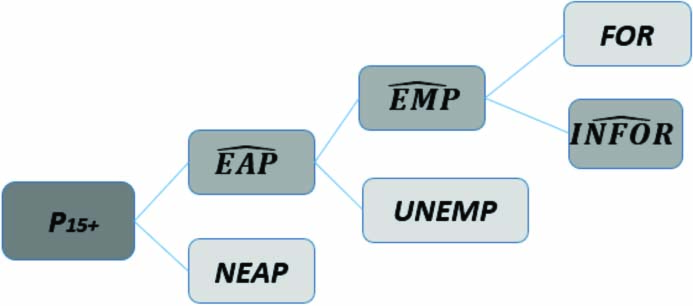
P15+: Population aged 15 and over. Group of people who at the time of the interview were 15 years old or more. EAP: Economically Active Population (estimated by statistical model developed for this purpose). It is made up of people aged 15 and over who had a link with an economic activity or who sought it out in the reference week, so they were either employed or unemployed. EMP: Employed Population (estimated by statistical model developed for this purpose). It includes people aged 15 and over who carried out some sort of economic activity for at least one hour in the reference week. It includes those employees who had a job but did not perform it temporarily for some reason without losing their employment relationship; also, it includes those who helped in any economic activity without receiving a salary or wage. FOR: Formal Employed Population. They are people aged 15 and over who, due to the context in which they work, are capable of invoking the legal or institutional framework that corresponds to their economic insertion on their behalf, either as an independent or subordinate worker. INFOR: Informal Employed Population (estimated by statistical model developed for this purpose). They are people aged 15 and over who, due to the context in which they work, cannot invoke the legal or institutional framework that corresponds to their economic insertion on their behalf; then, the entire spectrum of occupational modalities will be occupation or informal employment (either dependent or independent) on which this circumstance gravitates. It groups all the forms of informal employment together: The informal sector, paid domestic work for households, unprotected agricultural work and subordinate workers who, despite working in formal economic units, do it so in a manner which does not include social security. UNEMP: Unemployed Population. People aged 15 and over that, in the reference week, were looking for a job because they were not linked to any economic activity or work. NEAP: Non-Economically Active Population. People aged 15 and over who only carried out non-economic activities in the reference week and were not looking for a job [2].

1.2Small Area Estimation

Small areas are population subsets of a smaller size than those considered in the original design of a probability sample survey; they can be geographic areas or thematic domains that are not considered explicitly. Estimation techniques for small areas (SAE) are relatively novel statistical tools that allow estimating parameters without needing to develop any additional survey just by using combined and integrated multiple-purpose sources of information: surveys, censuses, administrative records, and others [3, 4, 5].

The main methods for estimating the general parameters of small areas are: the Empirical Best Linear Unbiased Predictor (EBLUP) based on the well-known area level model of Fay-Herriot by Fay and Herriot [6]; the Elbers method [7], called the ELL method and used by the World Bank; the empirical Best or Bayes (EB) method by Molina and Rao [8]; and other variants of the EB method to treat two-stage sampling or informative unit sampling, in Molina, Nandram, and Rao [9]. EBLUP is the method used in this research.

Table 1

Variables to be estimated

EAP		Employed		Informal
Auxiliary variable	Description	Auxiliary variable	Description	Auxiliary variable	Description
Economic dependency ratio	Population under 15 years old and 65 years old and over compared to the population of 15 to 64 years old	Economic dependency ratio	Population under 15 years old and 65 years old and over compared to the population of 15 to 64 years old	Proportion of the population aged 45 years old and over	Population aged 45 years old and over compared to 15 years old and over
Proportion of male population	Population aged 15 to 44 years old compared to the population aged 15 and over	Proportion of male population	Population aged 15 to 44 years old compared to the population aged 15 and over	Proportion of the population affiliated to IMSS or ISSSTE	Population affiliated to these institutions compared to the population aged 15 years old and over
Proportion of the population affiliated to IMSS or ISSSTE	Population affiliated to these institutions compared to the population aged 15 years old and over	Proportion of the population affiliated to IMSS or ISSSTE	Population affiliated to these institutions compared to the population aged 15 years old and over	Proportion of population benefiting from Seguro Popular	Population affiliated to this program compared to the population aged 15 years old and over

Note. Variables object of estimation and their corresponding auxiliary variables. IMSS, ISSSTE and Seguro Popular are governmental organizations that assist public health in Mexico.

1.3Data source

Currently, there is no data source which offers direct results of labor figures in Mexico at the municipal level; therefore, it has been chosen to use different combined information sources and apply SAE techniques.

On the one hand, the variables to be estimated were taken from the National Occupation and Employment Survey (ENOE); its statistical design guarantees accurate results at the national level, for each federative entity and for other geographic levels higher than those of the municipality. On the other hand, the 2010 Population and Housing Census, various administrative records of social security, indicators, indices, surveys and projections published from various public institutions in Mexico, were used to obtain auxiliary variables.

2.Method

The method proposed in this paper responds to the need for information on main labor characteristics: EAP, Employed Population (Employed) and Informal Employed Population (Informal) for all municipalities in Mexico since ENOE only provides available estimates of these characteristics at a national level, state, and for some cities. The method’s process can be summarized in the following steps:

1. Auxiliary variables
2. The small area model and the Mahalanobis distances
3. Probability distribution fitting
4. Spatial model generation
5. State value adjustments

2.1Auxiliary variables

To estimate the variables of interest, it was necessary to resort to other sources of information – which should be consistent with the reference dates, the observation unit and the ENOE’s analysis unit. The auxiliary variables, which are those that explain the variables being estimated, were obtained through these sources.

Due to this, firstly, an analysis of international experiences was carried out (this being under the premise of investigating which auxiliary variables have been used in similar exercises) [3, 10, 11, 12, 13, 14, 15]. Secondly, the searching and processing of the sources was carried out in order to have a set of auxiliary variables that allow a statistically adequate estimation.

In this way, an initial set of 12 auxiliary variables was considered – for which temporal and geographic reference adjustments were made to make them compatible with the information of the variables under study provided by ENOE. The variables were subjected to statistical analysis and tests to determine the final auxiliary variables by using the Forward Stepwise Regression method [16]. The auxiliary variables selected for their predictive power are described in Table 1.

2.2The small area model and Mahalanobis distances

The used predictor is derived from a mixed linear model which involves fixed effects, random effects, and random errors. In a first stage, it is assumed that the variable of interest is obtained by direct estimation θ^aD (Eq. (1)), which represents the value obtained in ENOE’s survey plus the random error due to sampling; in this equation and its consequents, the subscript a represents each municipality. In a second stage, it is assumed that the variable of interest is linearly related to a vector of auxiliary variables (Eq. (2)).

(1)

θ^a(D)=θa+ea

(2)

θa=xaT⁢β+va

The element xa indicates a vector of auxiliary variables and a=1,2,3⁢…⁢m where m is the total number of municipalities.

The estimator xaT⁢β^𝐹𝐻=θ^aS is known as the synthetic estimator, which was also applied to obtain estimates of labor figures when there is no ENOE sample in the municipality, or because the municipality was excluded as part of the model because it was considered to be an extreme value.

The element va is known as the random effect.

By replacing Eq. (2) in Eq. (1), a linking model is obtained and through this model, the BLUP (Best Linear Unbiased Prediction) model is obtained Eq. (3).

(3)

θ^a𝐵𝐿𝑈𝑃=xaT⁢β^+v^a

The values of β^ (Eq. (4)) are obtained considering that the variable of interest, as well as the auxiliary data, are kept at a small area level (totals per area, averages per area or percentages per area).

(4)

β^𝐹𝐻=[∑a=1mxa⁢xaTσ^v2+ψ^a]-1⁢[∑a=1mxa⁢θ^a(D)σ^v2+ψ^a]

An empirical predictor for Eq. (3) is the one provided by the EBLUP (Empirical Best Linear Unbiased Predictor) – one of the most widely used predictors of small areas.

The EBLUP estimator is a linear combination of the direct estimator and the synthetic estimator (Eq. (5)).

(5)

θ^a(EB)=γ^a⁢θ^a(D)+(1-γ^a)⁢θ^aS

In both components (direct estimator and synthetic estimator) the gamma weighting is applied (Eq. (6)).

(6)

γ^a=σ^υ2σ^υ2+ψ^a

Where ψ^a the variance of the survey is assumed to be known and the variance of the random effects σ^υ2 is obtained by computational recursive methods [17, 18].

In this way, the EBLUP model was applied to obtain the predictions of the labor figures when there is an ENOE sample in the municipality. The mathematical formula of EBLUP’s empirical predictor expresses that the estimates obtained under this model (the posteriori information in terms of Bayesian Inference) are a mix of what is observed from ENOE (the a priori information in terms of Bayesian Inference) and the obtained result from the synthetic model. The gamma weighting (Eq. (6)) results from dividing the variance of the random effects by the sum of the variance of the random effects plus the observed variance of the direct estimator of ENOE; therefore, if the variance of the survey is small when compared with the variance of the random effects, the gamma weight’s value will have a value close to one, and consequently the estimation of ENOE will have more weight in the EBLUP predictor; on the contrary, if the variance of the survey is large when compared with the variance of the random effects, the gamma weight will have a value close to zero and, therefore, the synthetic estimate will have more weight in the EBLUP predictor. Check Section 6.1.2 of Rao and Molina [19] as a reference on how to obtain the variance of the random effects and its estimator.

In this part of the method, all municipalities that register at least one sample unit of ENOE (1010 municipalities) were taken as an input. Thus, by obtaining a first SAE model, both the residuals and the value of the random effects were obtained for each of the to-be-estimated variables.

It is worth mentioning that, in this part, routines were developed to estimate the variance that was not possible to capture in the ENOE operation due to the fact that the municipality had only one Primary Sampling Unit (PSU); its estimation was made by fitting either a curve or a straight line according to the behavior of the municipalities that did have variance.

Once both the residuals and the value of the random effects had been calculated for each of the to-be- estimated variables the extreme points (outliers) were detected by calculating the Mahalanobis distances for each estimate. As the variables EAP and Employed were correlated, the residuals and the value of the random effects of each of the variables were combined to calculate the Mahalanobis distances.

Meanwhile, for Informal the distances were obtained exclusively by their residuals and their random effects.

Robust Mahalanobis distances were obtained by applying Rousseeuw’s Minimum Determinant of Covariance method [20] included in the R package.

2.3Probability distribution fitting

Once the Mahalanobis distances were calculated, routines were developed to adjust these values to different probability distribution functions. For each variable object of estimation, 6 different functions were used: Cauchy, Chi Square, Gamma, Weibull, Log Normal and Student’s t distribution. The best distribution for each of the to-be-estimated variables was selected on the basis of the best graphic adjustment, on the values of the Bayesian and Akaike criteria, and on the appliance of statistical tests for the goodness-of-fit. Once the distribution function for each of these variables of interest had been determined, probabilities for each Mahalanobis distance were calculated. When probabilities were obtained, they were ordered from lowest to highest, and those records whose value is greater than 0.10 and less than 0.25 were selected as candidates for evaluation in the next stage of the method’s process.

2.4Spatial model generation

Beginning from Tobler’s first geographical law (1970) “Everything is related to everything else, but closer things more so”, a possible spatial autocorrelation was considered for the to-be-estimated variables [21]. Moran’s Index was used, and it was concluded that the spatial distribution is far from being merely random. Consequently, a spatial component was included in the part that represents the random effects of the EBLUP model (Eq. (7)), generating a new model called SEBLUP.

(7)

υ=(Im-ρ⁢W)-1⁢u

In the above equation ρ is the spatial correlation coefficient; W is the matrix of the inverse of the distances between the municipal capitals (W is the proximity matrix and it contains the percentages of the inverse of the distances between the municipal capitals); u is a vector of error terms with zero mean and constant variance; Im, it is the m-row identity matrix. Equation (7) implies that υ has a new variance component with a variance-covariance matrix of the form of Eq. (8).

(8)

G⁢(θ)=σ^u2⁢[(Im-ρ⁢W)T⁢(Im-ρ⁢W)]-1

By doing γ^a′=zmT⁢G⁢(θ)^⁢zT⁢[z⁢G⁢(θ)^⁢zT+𝑑𝑖𝑎𝑔⁢(ψ^a)]-1 (where z are the elements of the random effect design matrix, generally diagonal matrices, and zm is a vector of size 1*m) we obtain the SEBLUP spatial model Eq. (9) [19, 22, 23].

(9)

θ^a(𝑆𝐸𝐵)=γ^a′⁢θ^a(D)+(1-γ^a′)⁢θ^aS′

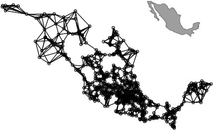
In order to build the W matrix, the Euclidean distances between the municipal capitals were measured in linear kilometers. Note that only the municipalities with a sample from which the model was constructed feature on the map (Fig. 2); later on, the reciprocal of these distances was calculated. Finally, the percentage that represents the reciprocal distance with each of its neighbors was determined for each municipality. The reciprocal was considered to give more weight to the neighbors who are geographically closer to the reference municipality than those who are further away.

Figure 2.

Distances between municipal capitals.

Matrix W of the proportions of the inverses from the distances used in the SAE model is a non-symmetric square matrix (figure in percentages which sum equals to 100). A real example of these values for six neighbors of each municipality of Aguascalientes state (who were input for the model’s construction) is shown in Tables 2a and b, and Table 3; in Table 2a and b, the neighboring municipalities that are part of Aguascalientes state are presented, while in Table 3 the figures of the neighboring municipalities that are not part of Aguascalientes state are shown.

Table 2

a. Municipalities within the state of Aguascalientes that neighbor each other
Municipality	San Francisco de los Romo	Rincón de Romos	San José de Gracia	Jesús María	Tepezalá	Aguascalientes	Pabellón de Arteaga
San Francisco de los Romo		12.58%	10.79%	14.27%	15.60%	14%	32.75%
Rincón de Romos	10.57%		12.88%		19.14%		16.25%
San José de Gracia	14.01%	19.91%		18.44%			19.67%
Jesús María	17.17%	11.11%	17.09%			20.99%	17.75%
Tepezalá	14.98%	21.87%					18.52%
Aguascalientes	19.84%		11.49%	24.73%			15.59%
Pabellón de Arteaga	28.76%	16.98%	13.30%	12.95%	16.95%
Calvillo			15.79%	19.24%		11.97%
Cosío		27.30%	9.19%		17.62%		10.84%

b. Municipalities within the state of Aguascalientes that neighbor each other
Calvillo	Cosío
	26.66%
14.09%	13.88%
15.90%
	19.66%
11.65%
	11.06%

Table 3

Municipalities outside of the state of Aguascalientes that neighbor the municipalities within the state of Aguascalientes

Municipality	Cuauhtémoc	Loreto	Encarnación de Díaz	Huanusco	Tabasco	Jalpa	Ojocaliente
San Francisco de los Romo
Rincón de Romos	14.50%
San José de Gracia
Jesús María
Tepezalá	11.04%	13.93%
Aguascalientes			16.69%
Pabellón de Arteaga
Calvillo				19.19%	21.77%	12.04%
Cosío	22.47%						12.58%

The map of Aguascalientes state and its municipal division is shown below (Fig. 3) as a reference for neighborhoods between municipalities.

Figure 3.

Municipalities of Aguascalientes state. Jalisco state and Zacatecas state are also depicted.

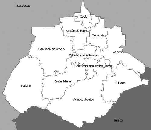
Figure 4.

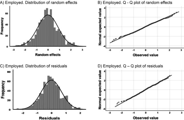
Frequency distribution graph and Q-Q plot. Through them, the normality of the random and residual effects for the Employed variable can be observed.

In this part of the process, the selected records (explained in Section 2.3) and the number of neighborhoods between neighboring or nearby municipalities – which may even be in different states, were required as an input. For each record, 4, 5 and up to 6 neighbors were used since they represent the national mean, mode and median of the geographic neighborhoods. The largest sample size, the highest spatial correlation, and compliance with the statistical assumptions were considered to select the best model out of the hundreds that were generated.

Once the best model had been selected by using the library “sae” from R [24], we proceeded to calculate the estimates of the municipalities that did not belong within this construction by using the synthetic component of the model for expected values and designing routines in R to the calculation of the Mean Squared Errors according to Section 6.2.2 of the “Small Area Estimation” book, by Rao and Molina [19]. Information from all the municipalities of the country was obtained in this way.

2.5State value adjustments

Mexico is divided into 32 states, and each of these is subsequently divided into municipalities. Once the estimates for all of Mexico’s municipalities have been calculated, they are grouped according to the state to which they belong to. This is done to adjust the sum of estimates for each of the municipalities to the value provided by ENOE at a state level. In this part of the method process, the Iterative Proportional Adjustment algorithm for two-dimensional tables is used [25].

3.Verification of assumptions

Through statistical and graphical tests, the following assumptions of the generated model were verified:

1. Multicollinearity: The correlation between the auxiliary variables is controlled.
2. Homoscedasticity: It is verified that the residuals show variances’ equality.
3. Normality of random effects: It is verified that the distribution of the random effects is normal.
4. Normality of residuals: It is verified that the distribution of the residuals is normal.

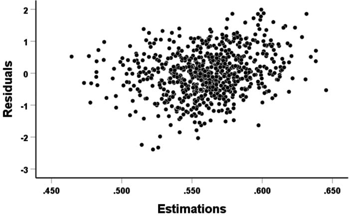
Indeed, in a visual manner for the Employed variable, bar graphs and quantile-quantile graphs were obtained – where it is observed that the random effects are approximately distributed according to a normal distribution (sections A and B of Fig. 4); the same happens with the residuals (sections C and D of Fig. 4). In addition, Fig. 5 shows the residuals’ dispersion through a graph that shows homoscedasticity.

Figure 5.

Homoscedasticity for the Employed variable.

To corroborate what was observed in the previous graphs, it was necessary to carry out the numerical tests of assumptions. In Table 4a and b obtained result are shown (W being the Shapiro-Wilk test, KS being the Kolmogorov test and JB being the Jarque-Bera test).

Table 4

a. Statistical tests of normality, homoscedasticity and multicollinearity
Estimation variable	Number of cases (municipalities)	Moran’s I [-1, 1]	K neighbors	Rho spatial correlation [-1.1]	Random effects p-value (%)
					W	KS	JB
EAP	760	0.207	6	0.69	30.9	23.2	41.8
Employed	760	0.195	4	0.68	1.2	2.2	16.1
Informal	796	0.308	4	0.811	90.5	43.2	77.8

b. Statistical tests of normality, homoscedasticity and multicollinearity
Residuals p-value (%)			Breusch Pagan homocedasticity p-value (%)	Multicollinearity Kappa information index
W	KS	JB
53.8	10.9	84.4	43.8	39.3
7.76	0.8	46.2	57.7	39.3
20.4	38.4	19.7	10.0	23.2

Figure 6.

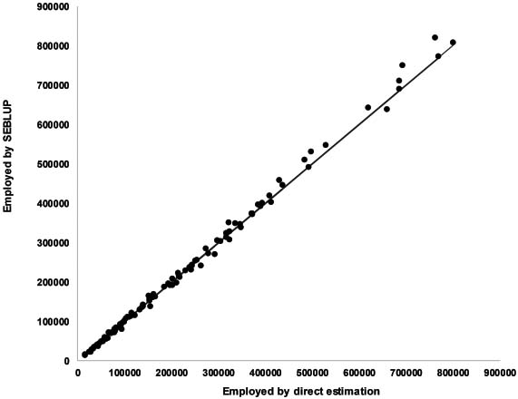
Total Employed 2018 SEBLUP contrasted against the direct estimate. Municipalities in which CV (ENOE) < 20%. CV means coefficient of variation.

Figure 7.

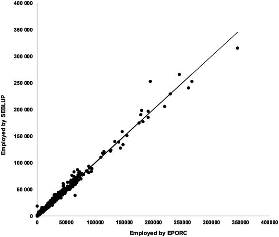
Total Employed 2018 SEBLUP contrasted against the EPORC estimate. Municipalities in which CV (ENOE) ≥ 20% and for those which were not sampled.

Figure 8.

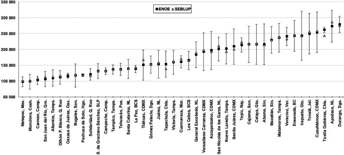
Employed Population. ENOE confidence intervals for municipalities with CV < 20% and SEBLUP ENOE estimates, first quarter of 2018. Of the 111 municipalities with CV < 20% according to the direct estimate of ENOE, the corresponding confidence intervals contain 104 estimates of SEBLUP, while seven were located outside the range. This graph, for scale reasons, only illustrates municipalities which population (ordered from smallest to largest) is located in the central part.

Figure 9.

Estimates of 2018 Employed Population for Aguascalientes’ municipalities.

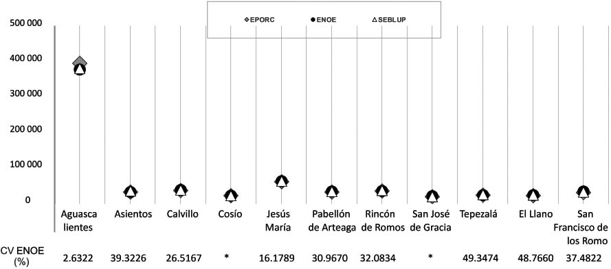
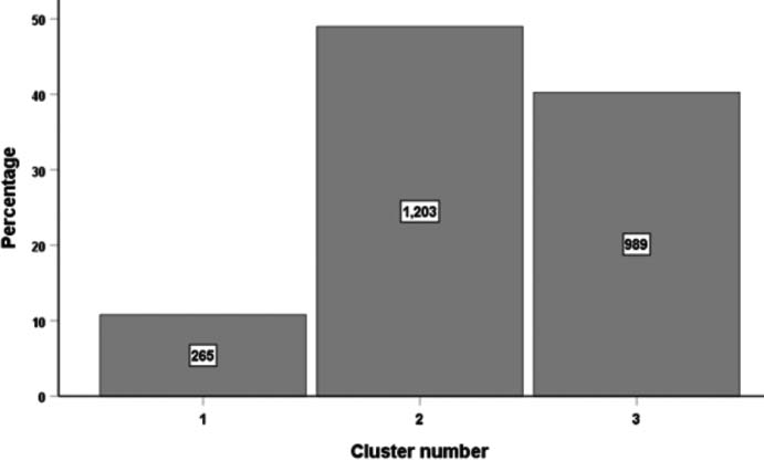
Figure 10.

Cluster integration for the Employed variable.

4.Results

The obtained results by SAE were divided into 2 groups to make comparisons. The estimates of the municipalities that had a sample in ENOE were located in the first group with a coefficient of variation less than 20%; in the second group were the estimates of the municipalities that did not have a sample in the survey, or if they did, their coefficient of variation was equal to or greater than 20%. The estimates of the first group were compared with the data obtained by direct estimation through ENOE. In Fig. 6 the Employed variable is compared for the first group. In contrast, the estimates of the second group were compared with the values calculated by applying the percentage structure of the 2010 Population and Housing Census (EPORC for its acronym in Spanish) to the figures at the federal entity level provided by ENOE. Figure 7 shows the comparison for the Employed variable for the second group. In Figs 6 and 7, the line at 45 degrees indicates equality in both values; it is observed that the estimates obtained by SEBLUP are close to both the estimates of the first group and the estimates of the second group. The equality of values is better appreciated in Fig. 6.

The confidence intervals of the estimates that were classified within the first group were calculated, that being the direct estimates obtained through ENOE; the measurements obtained by SAE were analyzed accordingly with these confidence intervals. Figure 8 shows the location of SAE’s estimates accordingly with the confidence intervals of the direct estimates. For scale purposes, only the intervals for the municipalities whose estimation is located in the central part (ordered from lowest to highest according to the direct estimate) are illustrated. Almost 94% of the measurements obtained by SAE fall within the confidence intervals of the direct estimates.

Figure 9 compares the three estimates for the Employed variable in all municipalities of a particular federal entity: The direct estimate through ENOE, the estimate calculated by applying the percentage structure of the 2010 Population and Housing Census (EPORC) to the state level figures provided by ENOE, and the estimate calculated by SAE. That so-called federative entity was selected to exemplify our model because of the low number of municipalities (in Mexico the number of municipalities per federal entity varies; while there are entities with only 5 municipalities, there are others with more than 200 municipalities). In the aforementioned Fig. 9 it can be seen that the results for the same municipality are very similar, so much so that the points get overlapped.

Cluster analyses were performed. For the Employed variable, 3 clusters were formed according to the percentage of Employed Population. Figure 10 shows the 3 formed clusters and the number of municipalities in each of them.

The first group shows the behavior of 265 municipalities that register rates from 90.9% to 96.8% with a median of 96.2%. In another group there are 1 203 municipalities with rates ranging from 98.5% to 99.9%, with a median of 99.4%. And, in a third group there are 903 municipalities with rates between 96.8% and 98.5%, and a median of 97.9%.

5.Conclusions

SEBLUP method was applied to calculate the estimates in all the municipalities of Mexico during 2018’s first quarter. The results were close to the direct estimates obtained through ENOE itself (for the municipalities that had a sample and which coefficient of variation is less than 20%) and the obtained estimates by applying EPORC to the figures by state provided by ENOE (for municipalities that did not have a sample in ENOE or which coefficient of variation was equal to or greater than 20%). These comparisons show that the used technique and predictor are acceptable for calculating the to-be-estimated variables at municipal level.

The municipalities of the central-south region are those that register the lowest values for the proportions of EAP compared to the population aged 15 years old and over and of Employed Population compared to EAP. Regarding the values’ precision estimated by the model, it is clearly appreciated that the coefficients of variation decrease as the sample size increases, and those obtained by SEBLUP are notably smaller than those of the survey. It is important to emphasize that ENOE was not designed to obtain figures at municipal level, for this reason the CVs are high and dispersed.

Information from different sources was used for the described method; from it, statistical models that have allowed calculating estimates for small areas of the Economically Active Population, Employed Population and Informal Employed Population were constructed.

The main source of information on labor figures in Mexico provides data at national and state level, and for some cities. However, municipal governments have an imminent need for this type of information at local or subnational levels.

Acknowledgments

We want to express our gratitude for the provided support in the preparation of this work to: The Deputy General Director of Statistical Infrastructure, Jorge E. Ochoa Setzer; the entire work team of the Statistical Process Development Department (particularly to César Bistrain Coronado, Josué R. Esquivel Balseca, Alfonso Millán Licona, Marco A. Vázquez Andrade, José R. Campos Luévano, José D. Loera Serna and Luis F. Salazar López). The points of view expressed in this article correspond to its authors and do not necessarily represent the opinion of the National Institute of Statistics and Geography.

References

[1]	National Institute of Statistics and Geography (INEGI) [homepage on the Internet]. Prevalencia de Obesidad, Hipertensión y Diabetes para los Municipios de México 2018; (2020) [updated 2020 Jul 21; cited 2020 Aug 3]. Available from: https://www.inegi.org.mx/contenidos/investigacion/pohd/2018/doc/a_peq_2018_nota_met.pdf.
[2]	National Institute of Statistics and Geography (INEGI) [homepage on the Internet]. Encuesta Nacional de Ocupación y Empleo (ENOE), población de 15 años y más de edad; [updated 2020 Sep 8; cited 2020 Sep 8]. Available from: https://www.inegi.org.mx/programas/enoe/15ymas/.
[3]	Kordos J. Development of small area estimation in official statistics. STATISTICS IN TRANSITION New Series. (2016) ; 17: (1): 105–32. doi: 10.21307/stattrans-2016-008.
[4]	United Nations Department of Economic and Social Affairs of the (UN DESA). Principles and Recommendations for Population and Housing Censuses. Rev. 3. New York: United Nations; (2017) .
[5]	Tzavidis N, Zhang L, Luna A, Schmid T, Rojas-Perilla. From start to finish: a framework for the production of small area official statistics. Journal of the Royal Statistical Society Serie A. (2018) ; 181: (4): 927–79.
[6]	Fay RE, Herriot RA. Estimates of income for small places: an application of james-stein procedures to census data. Journal of the American Statistical Association. (1979) ; 74: (366): 269–77. doi: 10.2307/2286322.
[7]	Elbers C, Lanjouw JO, Lanjouw P. Micro-level estimation of poverty and inequality. Econometrica Journal of the Econometric Society. (2003) ; 71: (1): 355–64. doi: 10.1111/1468-0262..
[8]	Molina I, Rao JNK. Small area estimation of poverty indicators. The Canadian Journal of Statistics. (2010) ; 38: (3): 369–85.
[9]	Molina I, Nandram B, Rao JNK. Small area estimation of general parameters with application to poverty indicators: a hierarchical bayes approach. The Annals of Applied Statistics. (2014) ; 8: (2): 852–85.
[10]	Molina I, Saei A, Lombardía MJ. Small area estimates of labour force participation under a multinomial logit mixed model. Journal of the Royal Statistical Society Serie A. (2007) ; 170: (4): 975–1000.
[11]	Münnich R, Burgard JP, Gabler S, Ganninger M, Kolb J. Small area estimation in the german census 2011. STATISTICS IN TRANSITION New Series. (2016) ; 17: (1): 25–40. doi: 10.21307/stattrans-2016-004.
[12]	Pusponegoro NH, Rachmawati RN. Spatial empirical best linear unbiased prediction in small area estimation of poverty. Procedia Computer Science. (2018) ; 135: : 712–18. doi: 10.1016/j.procs.2018.08.214.
[13]	Ramos R [Internet]. Indicadores sociodemográficos a nivel área pequeña para la Encuesta Intercensal 2015: Incorporación de efectos espaciales y temporales; 2015 [cited 2020 Feb 20]. Available from: https://www.inegi.org.mx/eventos/2017/conacyt/doc/p_RogelioRamos.pdf.
[14]	The EURAREA Consortium. PROJECT REFERENCE VOLUME. In: EURAREA, Enchancing Estimation Techniques to meet European Needs; (2004) .
[15]	The EURAREA Consortium. PROJECT REFERENCE VOLUME Vol. 3: SAS Programs and Documentation. In: EURAREA, Enchancing Estimation Techniques to meet European Needs; (2004) .
[16]	Rawlings JO, Pantula SG, Dickey DA. Applied regression analysis: A research tool. 2nd ed. New York: Springer; (1998) .
[17]	Pratesi M, Salvati N. Small area estimation in the presence of correlated random area effects. Journal of Official Statistics. (2009) ; 25: (1): 37–53.
[18]	Rao JNK. Small area estimation. 1st ed. Hoboken: Wiley; (2013) .
[19]	Molina I, Rao JNK. Small area estimation. 2nd ed. Hoboken: Wiley; (2015) .
[20]	Rousseeuw PJ, Van Driessen K. A fast algorithm for the minimum covariance determinant estimator. Technometrics. (1999) ; 41: (3): 212–23. doi: 10.1080/00401706.1999.10485670.
[21]	Tobler WR. A computer movie simulating urban growth in the detroit region. Economic Geography. (1970) ; 46: (supplement 1): 234–40. doi: 10.2307/143141.
[22]	Getis A, Ord JK. The analysis of spatial association by use of distance statistics. Geographical Analysis. (1992) ; 24: (3): 189–206. doi: 10.1111/j.1538-4632.1992.tb00261.x.
[23]	Marhuenda Y, Molina I, Morales D. Small area estimation with spatio-temporal Fay-Herriot models. Computational Statistics and Data Analysis. (2013) ; 58: : 308–25.
[24]	Molina I, Marhuenda Y. Sae: an R package for small area estimation. The R Journal. (2015) ; 7: (1): 81–98. doi: 10.32614/RJ-2015-007.
[25]	Hunsinger E [Internet]. Iterative Proportional Fitting for a Two-Dimensional Table. [cited 2020 Mar 31]. Available from: https://u.demog.berkeley.edu/∼eddieh/IPFDescription/AKDOLWDIPFTWOD.pdf.