
Improving the quality of disaggregated SDG indicators with cluster information for small area estimates
Abstract
The increasing needs for more disaggregated data motivates National Statistical Offices (NSOs) to develop efficient methods for producing official statistics without compromising on quality. In Indonesia, regional autonomy requires that Sustainable Development Goals (SDGs) indicators are available up to the district level. However, several surveys such as the Indonesian Demographic and Health Survey produce estimates up to the provincial level only. This generates gaps in support for district level policies. Small area estimation (SAE) techniques are often considered as alternatives for overcoming this issue. SAE enables more reliable estimation of the small areas by utilizing auxiliary information from other sources. However, the standard SAE approach has limitations in estimating non-sampled areas. This paper introduces an approach to estimating the non-sampled area random effect by utilizing cluster information. This model is demonstrated via the estimation of contraception prevalence rates at district levels in North Sumatera province. The results showed that small area estimates considering cluster information (SAE-cluster) produce more precise estimates than the direct method. The SAE-cluster approach revises the direct estimates upward or downward. This approach has important implications for improving the quality of disaggregated SDGs indicators without increasing cost.
The paper was prepared under the kind mentorship of Professor James J. Cochran, Associate Dean for Research, Prof. of Statistics and Operations Research, University of Alabama.
1.Introduction
The increasing needs of evidence-based policy making underpins the increasing demand for official statistics [1]. National Statistical Offices (NSOs) play a prominent role in providing information for various aspects such as business and policy decision, public discussion and scientific research [2]. NSOs are demanded to produce more disaggregated, timely, and diversified statistics without compromising on quality. With limited resources, NSOs need to find an efficient way to achieving this purpose [3].
Indonesia has a decentralized governance system called ‘regional autonomy’. This system provides authority to local (provincial and district, with district being the lower level) governments to manage their regions for their own development. As a consequence, official statistics are needed to monitor regional developments up to the district level. BPS (Statistics Indonesia), the Indonesian NSO, is responsible for providing official statistics up to the district level through its regular surveys.
The regional autonomy system implies that Sustainable Development Goals (SDGs) targets are not merely adopted in the national development plan, but also integrated into local development plans. According to the regional autonomy system, each district in Indonesia is an important policy maker for the nation’s development.
Indonesia has a strong commitment to achieve the SDGs, including in the field of family planning. Target 3.7 of the SDGs declares that universal access to sexual and reproductive health-care services, including for family planning, information, and education, should be achieved by 2030. This target also mandates that reproductive health should be integrated into national strategies and programmes by that year as well. In the National Medium Term Development Plan (RPJMN) of Indonesia, the modern method contraception prevalence rate (mCPR) is targeted at 63.41% in 2024, while unmet needs for family planning are expected to decline to 7.4% by 2024.
Indicators for family planning targets are normally derived from the Indonesia Demographic and Health Survey (IDHS). The IDHS is conducted every five years with collaboration of the Indonesian National Population and Family Planning Board (BKKBN), Statistics Indonesia (BPS), and the Ministry of Health, which collects information about fertility, family planning, maternal and child health, etc. The most recent update of the IDHS in 2017 covers 1,970 census block samples in urban and rural areas and 47,963 successfully interviewed households. In the interviewed households, 49,627 eligible women and 10,009 eligible men were interviewed completely.
The 2017 IDHS used a two-stage stratified survey designed to produce estimates at national and provincial levels. Therefore, there are gaps for district level policies. One of alternative ways to fill these gaps is by increasing the sample size in the survey. However, this approach would be very costly and resource-intensive. Other strategies are needed to disaggregate the indicator statistics without increasing costs and the respondent’s burden.
The Small Area Estimates (SAE) method has been considered as a more cost-effective strategy [4]. Some studies also point out that SAE enables more reliable estimation of small areas by utilizing auxiliary information from other sources. This method can artificially increase the effective sample size and thus increase the precision of estimation [5].
Statistical techniques for SAE are diverse. Model-based is a frequently preferred method, where the specific area statistics are estimated from the regression between response variable from survey and auxiliary information from administrative data or census [6]. On the other hand, the Empirical Best Linear Unbiased Predictor (EBLUP) method is an indirect way to predict small area parameters. However, standard EBLUP uses a synthetic model that ignores area random effects for non-sampled areas [7]. As a result, the resulting estimates are distorted into a single line of the synthetic model and may result in considerable bias [8].
2.Methodology
In this paper, similarities among particular areas were used to estimate area random effects for non-sampled areas. This approach was used to estimate the contraception prevalence rate (CPR) at district level in the North Sumatera province. From 33 districts in North Sumatera, there are 6 districts that were not sampled in 2017 IDHS. The idea of incorporating cluster information into the standard EBLUP has been proposed by Anisa et al. [9]. This approach was modified in several ways: 1) partitioning around medoids algorithm was used to generate clusters. This algorithm will be explained later; 2) a logit transformation was used to ensure that CPR estimates fall between 0 and 1; and 3) the area level model was used rather than unit level model.
Data was acquired for the CPR in North Sumatera province from the 2017 IDHS and auxiliary variables from the Family Planning Coordinating Board of North Sumatera. To eliminate the scale effects, these auxiliary variables were transformed into standardized values. These auxiliary variables were only available at the district level. Table 1 lists the auxiliary variables used in this study.
Table 1
Lists of auxiliary variables
| No. | Variable | Description | Unit of measure |
|---|---|---|---|
| 1 | Z | Number of active acceptors | Person |
| 2 | Z | Number of family planning clinics | Unit of clinics |
| 3 | Z | Number of family planning institution | Unit of institution |
| 4 | Z | Number of pre-prosperous and 1 | Unit of family |
These auxiliary variables were used in identifying clusters and estimating the CPR using the SAE model. For the clustering process, the Human Development Index (HDI) was also considered so districts could be grouped based on their development levels.
This paper employs partitioning around medoids (PAM) algorithm to generate clusters. A medoid is simply the object from a cluster with the minimum average distance to all other objects in the cluster. Using this procedure,
The advantage of PAM is that it is less sensitive to outliers. As in
Cluster information is further incorporated into the standard SAE model. Cluster information is utilized to estimate area random effects for non-sampled areas, which can be written as:
where
This paper used the CPR as an indicator to be estimated and must take a value in the interval [0, 1]. A logit transformation was used to ensure that the CPR estimates fall between 0 and 1.
In particular,
where
Finally, the standard area level model is modified as follows:
• Model for population:
• Prediction model for sampled area:
• Prediction model for non-sampled area:
where
If
where
This paper employs R software to derive estimates of
is constructed using Bootstrap method (see [14, 15]).
Figure 1.
Number of clusters using elbow method.
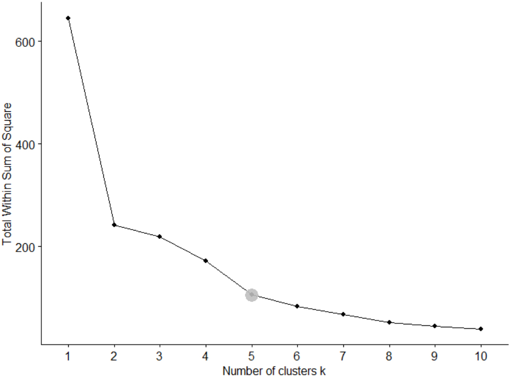
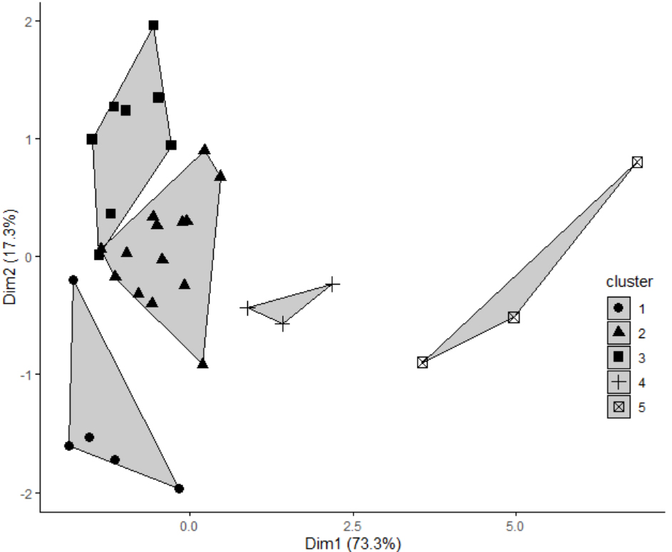
Figure 2.
Clustering result using partitioning around medoid (PAM) algorithm.
3.Results
Figure 1 depicts the resulting total within the sum of squares as a function of the number of clusters. Using the elbow method, the number of clusters was selected for which adding another cluster does not substantially decrease the total within the sum of squares. The figure shows that the total within the sum of squares decreases substantially when up to five clusters are used. Adding clusters at this point does not reduce the total within sum of square substantially. Six clusters would reduce the total within sum of squares by 16.47 units, while five clusters would reduce the total within sum of squares by 27.45 units. Thus, it was chosen to identify five clusters. Figure 2 visualizes the generated clusters derived using the PAM algorithm. This figure clearly shows that the five clusters are generally well-separated.
Table 2
Cluster of districts in north sumatera province
| Cluster | Number of cluster members | Districts |
|---|---|---|
| 1 | 5 | Nias, Nias Selatan, Pakpak Bharat, Nias Utara |
| 2 | 14 | Mandailing Natal |
| 3 | 8 | Toba Samosir, Samosir |
| 4 | 3 | Asahan, Simalungun, Serdang Bedagai |
| 5 | 3 | Deli Serdang, Langkat, Medan |
Note:
Figure 3.
Comparison of 95% confidence interval for the direct estimates and SAE-cluster estimate.
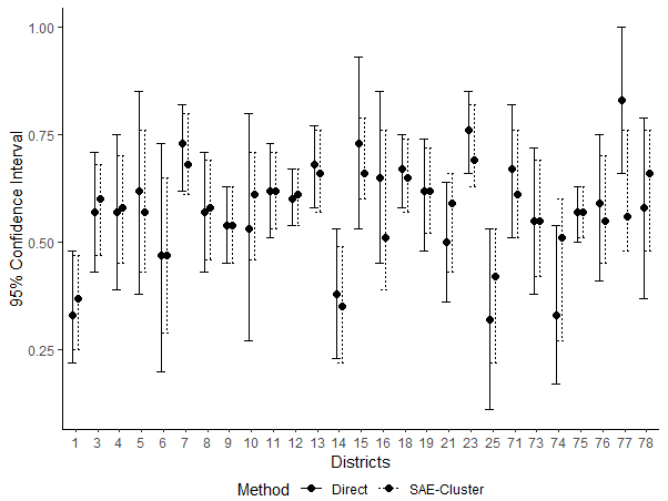
Figure 4.
Comparison of the spatial distribution for the direct estimates and SAE-cluster estimates.
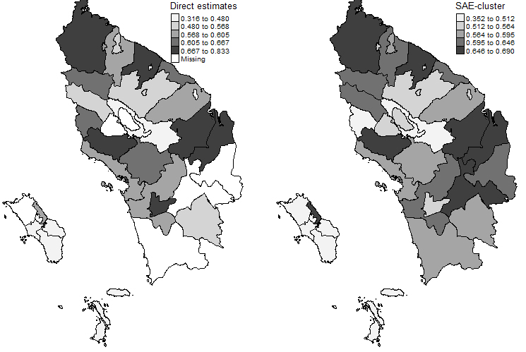
Table 2 presents the members of each cluster. Cluster 1 includes five districts; this includes one non-sampled district (Nias Utara). This cluster has the lowest development and family planning status. Cluster 2 consists of fourteen districts, including three non-sampled districts: Mandailing Natal, Padang Lawas Utara, and Labuhanbatu Selatan. This cluster has a moderate development and a moderate family planning status. Cluster 3 consists of eight districts, including two non-sampled districts: Samosir and Tanjungbalai. This cluster has a lower family planning status. Cluster 4 and cluster 5 each have three members. There is no non-sampled district in either cluster 4 or cluster 5. The districts in cluster 4 (Asahan, Simalungun, and Serdang Bedagai) and cluster 5 (Deli Serdang, Langkat, and Medan) generally have a higher family planning status.
The results from above clusters were further utilized to estimate area random effects for non-sampled areas
• Prediction model for sampled area:
• Prediction model for non-sampled area:
A comparison between direct estimates and small area estimates that incorporate cluster information (SAE-cluster) is presented in a 95% confidence interval form in Fig. 3. The point in the middle of interval represents the corresponding point estimate of CPR, and the upper and lower limits of each interval respectively represent the upper and lower bounds of the corresponding 95% confidence interval for CPR (the SAE-cluster model revises the direct estimates). Confidence intervals of the SAE-cluster were generally shorter than the direct estimates. This suggests that the SAE-cluster model produces more precise estimates than the direct method.
A spatial distribution of the CPR estimates using direct estimation and SAE-cluster estimation are provided in Fig. 4. Missing values in direct estimates occur because some areas were not sampled in the 2017 IDHS. This issue is well handled by the SAE-cluster approach using information from sampled areas within the same cluster. The SAE-cluster approach revises the spatial distribution of CPR estimates in North Sumatera province and changes the relative position of several districts.
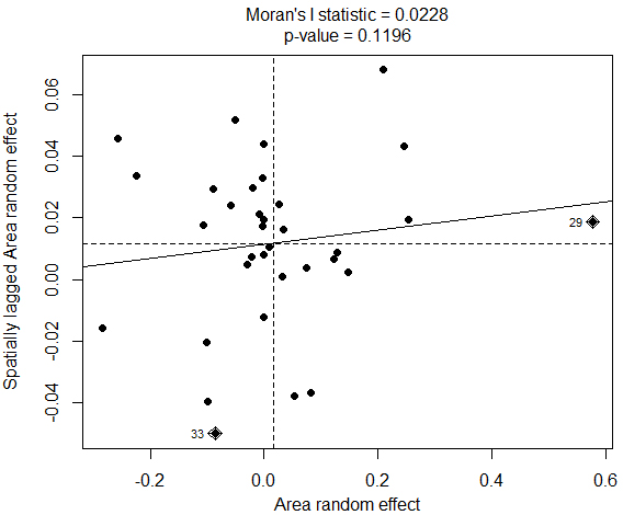
Another approaches have been proposed to handle the issue of non-sampled area. One of the frequently preferred method is the Spatial EBLUP (see [16, 17, 18, 19, 20]). This method utilizes spatial dependencies among regions to derive estimates for sampled areas as well as non-sampled areas. However, this approach is not applicable in this study since the Moran’s I test indicated that the area random effects are not spatially correlated (Fig. 5).
Figure 5.
Moran’s scatterplot of area random effect.
4.Conclusion
Incorporation of cluster information into small area estimation offers two advantages. First, it enables the sampled small areas to be estimated reliably. It enhances the precision of the estimates substantially. Hence, it addresses the issue of small samples at the district level. Second, it serves as a procedure for producing superior estimates of area random effects for non-sampled areas that support the development and assessment of comprehensive policy-making. This approach can help NSOs to meet the needs of more disaggregated statistics without increasing costs since this approach uses existing available data sources.
Acknowledgments
The authors are deeply indebted to Professor James J. Cochran for his warm mentoring, valuable advice and thoughtful guidance during the re-drafting process of this paper. Deep thanks are also expressed to the United Nations Economic and Social Commission for Asia and the Pacific (UNESCAP) for the opportunity to develop this paper and to contribute to global statistical community. Finally, sincere gratitude is expressed to BPS-Statistics Indonesia in supporting the study and providing data for it.
References
[1] | Round JI. Assessing the demand and supply of statistics in the developing world: some critical factors. PARIS21 Discussion Paper No.4. May (2014) : 1–20. |
[2] | Struijs P, Braaksma B, Daas PJH. Official statistics and big data. Big Data Soc. April-June (2014) : 1–6. |
[3] | Yazdani A, Van Halderen G. Integrated statistics: a journey worthwhile. ESCAP Stats Brief. (2019) ; (19): 1–6. |
[4] | ADB. Introduction to Small Area Estimation Techniques: A Practical Guide for National Statistics Offices. (2020) : 99. |
[5] | Rao JNK. Small-Area Estimation. Wiley StatsRef Stat Ref Online. (2017) : 1–8. |
[6] | Kordos J. Development of small area estimation in official statistics. Stat Transit. (2014) ; 17: (1): 105–132. |
[7] | Saei A, Chambers R. Empirical Best Linear Unbiased Prediction for Out of Sample Areas Southampton Statistical Sciences Research Institute Methodology Working Paper M05/03. March (2005) . |
[8] | Anisa R, Kurnia A, Indahwati. Cluster information of non-sampled area in small area estimation. IOSR J Math. (2014) ; 10: (1): 15–19. |
[9] | Anisa R, Notodiputro KA, Kurnia A. Small Area Estimation for Non-Sampled Area Using Cluster Information and Winsorization with Application to BPS Data. In: Proc ICCS-13. Bogor; (2014) : pp. 453–462. |
[10] | Sarda-Espinosa A. Time-series clustering in R using the dtwclust package. R J. (2019) ; 12: (2013): 1–40. |
[11] | Hastie T, Tibshirani R, Friedman J. The Elements of Statistical Learning. New York: Springer; (2008) . |
[12] | Cox DR, Snell EJ. Analysis of Binary Data. Boca Raton: Chapman & Hall/CRC; (1989) : 253. |
[13] | Eurostat. Guidelines on small area estimation for city statistics and other functional geographies. Luxembourg: Publications Office of the European Union; (2019) . |
[14] | Agresti A, Franklin C, Klingenberg B. Statistics: The Art and Science of Learning from Data. Fourth Ed. Essex: Pearson; (2018) : 817. |
[15] | Rao JNK. Jackknife and bootstrap methods for variance estimation from sample survey data. Int J Stat Sci. (2009) ; 9: (2009): 59–70. |
[16] | Moura FAS, Migon HS. Bayesian spatial models for small area estimation of proportions. Stat Model. (2002) ; 2: (3): 183–201. |
[17] | Rao JNK, Molina I. Small Area Estimation. Second Ed. Encyclopedia of Survey Research Methods. New Jersey: John Wiley & Sons, Inc; (2015) : 451. |
[18] | Law J. Exploring the specifications of spatial adjacencies and weights in bayesian spatial modeling with intrinsic conditional autoregressive priors in a small-area study of fall injuries. AIMS Public Heal. (2016) ; 3: (1): 65–82. |
[19] | Kubacki J, Jedrzejczak A. Small area estimation of income under spatial SAR model. Stat Transit New Ser. (2016) ; 17: (3): 365–390. |
[20] | Pusponegoro NH, Rachmawati RN. Spatial empirical best linear unbiased prediction in small area estimation of poverty. Procedia Comput Sci. (2018) ; 135: : 712–718. |

