
A monthly spatio-temporal modelling of patterns for children on maintenance grant in Namibia
Abstract
BACKGROUND:
Child support grant (CSG) is one of the social protection strategies which is today widely seen as an intervention contributing to poverty reduction. However, despite substantial expenses, it has been documented that Namibia’s social protection benefits do not reach intended beneficiaries in an efficient manner.
AIMS:
This study aims to determine factors associated with spatial and temporal variation in maintenance child grant and as well as identify regions with elevated incidence rate ratios of maintenance grant in Namibia.
METHODS:
We fitted a Bayesian spatio-temporal regression model on maintenance grant data available over 9 years in Namibia.
RESULTS:
The number of children on grant has almost tripled between March 2007 and October 2015 (it changed from 50596 in 2007 to 132840). Unemployment and orphanhood were significantly associated with the incidence rate ratio of maintenance grant (CI:(1.634, 2.627) and CI: (1.000, 1.004), respectively. The adjustment of measurement error in orphanhood through the Berkson error model has ensured the stability of its effect.
CONCLUSIONS:
This study has shown the strength of using measurement error models for analysing child grant data. Furthermore, the study has demonstrated that the northern regions of Namibia have the highest child incidence rate ratio of maintenance grant whereas the regions in central and south are at low incidence rate at present. The maps produced in this study can be particularly helpful in allocating efficiently limited resources in poor settings.
1.Introduction
Social protection, which is defined as public actions taken in order to reduce levels of poverty and vulnerability in a society, consists of social insurance; labour market regulation; and social assistance [1, 2]. The later includes tax financed policy instruments such as cash transfer programs to support old, orphans and other vulnerable persons.
Cash transfer programs have become widely popular in developing countries, particularly in Latin America, and have been adopted by more than 30 countries since they were first introduced in the 1990s” [3, 4].
About a decade ago, the sub-Saharan Africa had almost 43 million children under the age of 18 who had lost one or both parents due to various causes that include AIDS, conflict or other, needing approximately US$1.4 billion to provide for these orphans [5, 6].
There are two models of social protection in sub-Saharan Africa. Southern Africa social protection model is based on social assistance programs that are policy and rights based of citizens, while in middle Africa, social protection model is based on projects that are intended to respond to emergencies related issues [1, 7].
Child support grant (CSG) is one of the social protections which is today widely seen as a key factor contributing to poverty reduction interventions and means to reduce vulnerability to social, natural and economic shocks and stresses [8]. Cash transfer programs where child support grants fall was found to be a global and national approach to reduce poverty and maintain and accelerate progress across a range of Millennium Development Goals (MDGs) [9]. Investing in social protection system contributes to the improved income and outcomes at an individual and family level. There is good evidence of schemes providing recipients with greater income security, although the extent of the impacts depends on the level of investment” [10].
Further, such child support grants can be given to targeted beneficiaries because of identified needs. Such support might be conditional or unconditional aimed at encouraging access to critical services such as health or education services to individual children [11, 12]. Also, it was established that the CSG program does not only benefit children, it also contributes to positive outcomes on caregivers and at households; and adds to household income and reduces poverty among grant-recipient households [13].
Other evidence suggests that while such support has been targeting poor households in general, it had also contributed positively to the household consumption that results into reduced poverty [13, 14]. However, such results depend on the amount allocated to such benefits and mind sets of beneficiaries towards the program responses [14]. Other positive findings relating to CSG include positive results on young children development and promotion of safe practices for adolescents [13].
The rights of children to social protection are well documented in the Convention on the Rights of the Child (CRC). The CRC states that children have the right to social security, to adequate standards of living and they are provided through Social protection measures. According to the CRC, children have the right to social security [15]. Namibia is one of the few developing countries that has implemented the social protection system including CSG program for children in need of care and protection.
Namibia’s social protection landscape is rich as compared to other Sub-Saharan African countries. It has large social protection programs which form the basis of social assistance in the country [16]. The landscape includes public spending on old age pensions, war veterans’ grants, maintenance grants, vulnerable grants, foster parents’ grants, and disability grants for adults and children [16]. But it is important to emphasize that, “the outcomes of the schemes depend on the design, institutional capacity of the government, implementation mechanisms, costs, and the political acceptability of the measures” [17].
Namibia exceeds the average spending on public transfers for Sub-Saharan African countries in overall spending on direct transfers. Spending on direct transfers is higher than the average for Sub-Sahara African countries and comparable to the average for developing countries. Child support grants are intended to benefit children and are typically provided through primary caregivers who might also be classified as poor [16].
There are four types of social grants targeting children administered by the Ministry of Gender Equality and Child Welfare as one of the government entities [18]. The Child Maintenance Grant provides support to children with either a disabled parent, a parent receiving an Old Age Pension grant, a parent who is absent due to death or imprisonment or a child from poor household. This is a means tested grant, with the threshold for an applying parent set at less than a gross income of N$1200 on monthly basis. The Foster Care Grant targets children who were placed in the in the temporary care of foster parents by the Children’s Court. A special maintenance grant for children under the age of 16 who are living with disabilities. The number of children receiving CSGs has increased significantly from 19 711 children in 2004/2005 to 375 888 in 2018/2019 [19].
The CSG program is in line with poverty eradication which is one of the Sustainable Development Goals (SDG). Countries are mandated to report child poverty, end extreme child poverty and half child poverty according to national definitions by 2030 [20]. Henceforth, Namibia has shifted from focusing only on providing child support grants to orphans and Vulnerable children due to HIV/AIDS to the broader group of children including children from poor household [18].
Various studies have demonstrated that Child Support grants contribute to poverty reduction, nutrition, health and education [18, 21]. However, despite substantial expenses, it has been documented that social protection benefits do not reach beneficiaries in an efficient and effective way [22]. Moreover, a qualitative assessment of the effectiveness of the social protection system in Namibia revealed that poor children continue to face difficulties to access critical services that can lead them out of poverty [23]. Many other studies have focused on other aspects of child welfare that include cost of childcare [5], child health [24], child maternal mortality [25], child mortality [26], and child maltreatment [27] and hence ignoring the spatial and temporal variations of child grants. Although it is known to some extend that unemployment, orphanhood and child support are not equally spatially distributed, very little analyses that employ techniques capable of accounting for spatial and temporal variations in distribution of child grant are found in literature. The Bayesian approach is one of the statistical modelling methods which originated in disease mapping but has been lately employed in other fields that include epidemiology [28, 29], demography (Sartorius et al. [26, 30, 31]; and sociology [27, 31, 33]. It helps in assessing the spatial pattern of an event and identifying areas characterized by unusually high or low relative risk [34]. In addition to the evaluation of spatial trends, it is worthy investigating the temporal variation of an event which may be equally important in accounting for its variability distribution.
Data on maintenance grant, which is one of the forms of child grant, were available at regional level over 9 years in Namibia. Therefore, the aim of this study is to fit a Bayesian regression model capable of accounting for fixed, spatial and temporal effects and as well as identifying regions with elevated incidence rate ratios of maintenance grant in Namibia
This paper is structured as follows. Section 1 (introduction) presents the background to maintenance grant, the statement of the research problem and its objectives. In Section 2 (Methods), we begin with a short description of the setting. Furthermore, we described the dataset to be used in the research. Finally, we presented the statistical methods to be employed to analyse the data. Section 3 (Results) presents the results and their interpretations. Section 4 (Discussion and conclusions) discusses the findings in relation to other similar studies, presents the strengths and limitations of the study, and finally provides some recommendations.
2.Methods
2.1Setting
Namibia is in the south-western part of Africa. It shares borders with Zambia in northeast and Angola in the north, Botswana in the east and South Africa in southeast and Atlantic Ocean in the west. Though Namibia is among the largest countries with surface area of 824,292 km
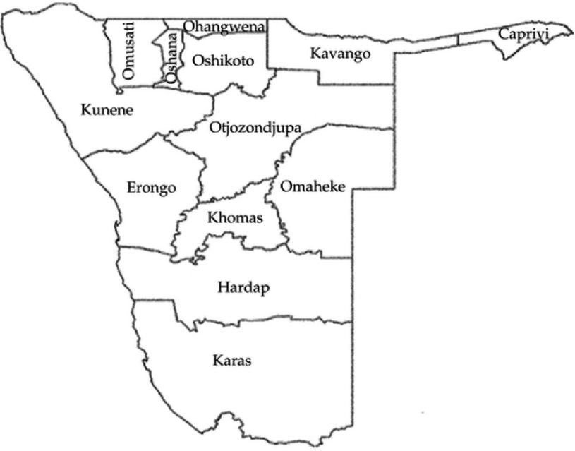
Figure 1.
Namibia Regional map.
2.2Data and variables
As neighborhood proxies, we used the 13 regions instead of the current 14 regions. The choice of using the old administrative map was dictated by the fact that data on the number of children receiving maintenance grant scheme were mostly recorded using the 13 regions. The regional boundaries shapefiles were obtained from the Namibia Statistics Agency (NSA).
Maintenance grant is a financial support for a child who is under the age of 18 with one of the biological parents earning less than N$1000.00 per month and with one or more of the following conditions: the other parent has died, or the other parent receives an old-age pension or a disability grant, or is unemployed, or the other parent is in prison for six months or longer. Thus, these conditions can be perceived as some of the factors influencing whether a parent can receive or not a maintenance grant. Due to lack of a database capturing and storing this information on all these variables, this study only used unemployment rate and orphanhood to account for some of the variability in maintenance grant.
Unemployment: Average unemployment rate (both sexes) for each region from 2010 to 2015 was obtained for the Namibia labour force surveys and Namibia 2011 population and housing census.
Orphanhood: The percentages of households with one or more orphaned children aged below 18 years in each region for the year 2001, 2011, and 2015 were extracted from Namibia 2001, 2011 population and housing census, and Namibia 2015/16 inter-census demographic survey respectively.
The outcome variable or response variable was the number of children receiving maintenance grant. Monthly data of children receiving maintenance grant for 9 years (from 2007 to 2015), was obtained from the Ministry of gender equality and child welfare and were used to capture temporal trends.
In the Ministry of gender equality and child welfare database, for each year, counts of number of children on the maintenance grant for January and February were combined and those of November and December were combined as well. To avoid inconsistency in the data, we excluded January, February, November and December in our analysis.
2.3Statistical analysis
The outcome variable was the monthly count of children who received child grant in Namibia during the period of the study (2007 to 2015). A conditionally independent Poisson distribution was used based on the month count of children on the maintenance grant scheme in each region for 72 months:
(1)
where
We are particularly interested in: (1) a model with only covariates (Non-spatial Poisson regression model), (2) a model with covariates and spatial random effects (spatial Poisson regression model), (3) a model with covariates, spatial temporal, and spatio-temporal interaction random effects (spatio-temporal Poisson regression model) and (4) a model with all previous components with covariate error model (spatio-temporal Poisson regression model adjusting for measurement errors).
2.3.1Non-spatial poisson regression model
Non-spatial Poisson model assumes that the variation in log – incidence rate ratio is the sum of variation due to covariates that include unemployment and orphanhood and the extra-variation attributed to the influence of region
(2)
where
2.3.2Spatial poisson model
To Eq. (2), we added unstructured and structured spatial effects to account for the spatial heterogeneity or overdispersion and the spatial effect, respectively. That is,
(3)
We specified a normal distribution
(4)
where
2.3.3Spatio-temporal poisson model
To build the spatio-temporal model we added a temporal component (
(5)
where
2.3.4Parametric trend
The parametric formulation extends Eq. (3) as follows:
(6)
where
2.3.5Nonparametric dynamic trend
The advantage of using nonparametric approach is that it helps relaxing the linearity constraint imposed on temporal differential trend
(7)
where
In this study, we have used the second approach, which is described below
(8)
where the parameter vector
Hence, the structure matrix is written in the following form
2.3.6Spatio-temporal Poisson model adjusting for measurement error
The extension of Eq. (8) to add a Berkson error model followed the specification provided in [38]. That is,
(9)
where an adjusted mismeasured covariate,
Table 1 gives the summary of the models fitted in this study.
Table 1
Regression models to be fitted
| Regression model | Fixed effect | Spatial component | Temporal component | space-time component | Error model |
|---|---|---|---|---|---|
| 1. Non-spatial |
| – | – | – | – |
| 2. Spatial |
|
| – | – | – |
| 3. Parametric |
|
|
|
| – |
| 4. Non-parametric 1 |
|
|
| – | – |
| 5. Non-parametric 2 |
|
|
|
| – |
| 6. Non-parametric 3 |
|
|
|
|
|
3.Results
3.1Exploratory results
Table 2
Monthly total number of children receiving maintenance grant in Namibia from 2007 to 2015
| Year | |||||||||
|---|---|---|---|---|---|---|---|---|---|
| Month | 2007 | 2008 | 2009 | 2010 | 2011 | 2012 | 2013 | 2014 | 2015 |
| March | 50596 | 77363 | 88420 | 96432 | 107894 | 117815 | 110739 | 126209 | 131347 |
| April | 54262 | 78816 | 89292 | 115154 | 108057 | 118678 | 122064 | 126308 | 130612 |
| May | 54238 | 80170 | 89589 | 99035 | 113530 | 114925 | 122370 | 126592 | 128903 |
| June | 54678 | 81300 | 90920 | 100103 | 103566 | 115156 | 122554 | 126930 | 131230 |
| July | 58637 | 82090 | 91443 | 88383 | 111949 | 115772 | 122419 | 127694 | 134099 |
| August | 62721 | 82284 | 90412 | 102156 | 119349 | 118067 | 122823 | 127995 | 135293 |
| September | 65064 | 83384 | 91461 | 102250 | 113787 | 118913 | 122854 | 128529 | 134125 |
| October | 67699 | 84570 | 93006 | 111517 | 115400 | 108359 | 124164 | 128657 | 132840 |
Table 2 provides the total number of children receiving maintenance grant every month from 2007 to 2015. Note that January February, November and December were removed from the study period for the reason earlier mentioned. It appears that there exist some variations between total number of children on maintenance scheme reported monthly. Also, it can be deduced that the number of children on grant has almost tripled between March 2007 and October 2015 (i.e. the number of children on grant changed from 50596 to 132840).
Figure 2.
Spatial distribution of unemployment rates over the period 2010–2015.
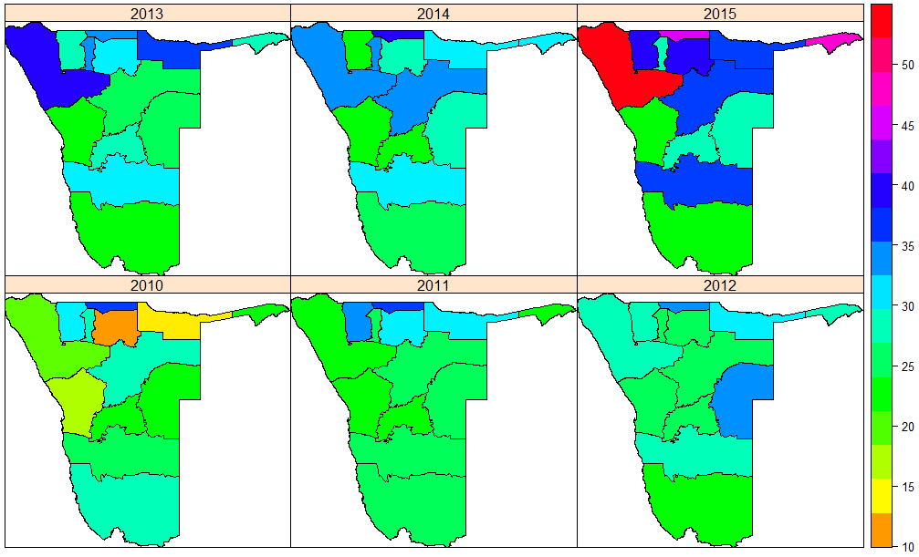
Figure 3.
Spatial distribution of orphanhood (% of households with at least one orphaned child aged below 18 years) for year 2001, 2011, and 2015.
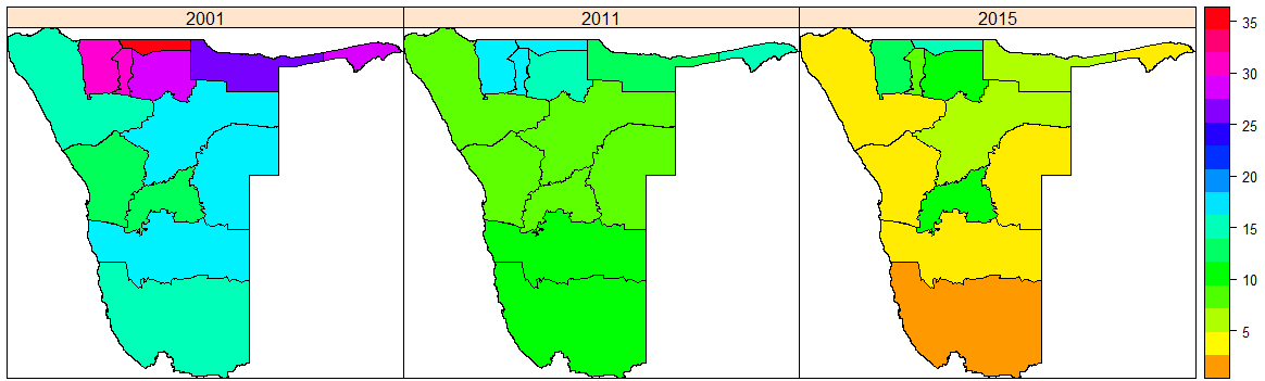
Figure 2 shows the spatial distribution of unemployment rates from 2010 to 2015. It can be noted that unemployment fluctuated between 10% and approximated more than 50% over the study period. Moreover, the figure showed that regions in the northern part of Namibia had high unemployment. Figure 3 displays the spatial distribution of households with at least one orphaned child aged below 18 years (in %) for year 2001, 2011, and 2015.
This figure not only revealed that the percentages of households with at least one orphaned child aged below 18 years varied among regions, but it also indicated that orphanhood oscillated over years. Again, the regions in the northern part of Namibia had more children aged below 18 years who had lost one or both parents as compared to the regions in the other parts of Namibia.
3.2Model selection
After fitting the six Bayesian Poisson regression models, we selected the best model using the Deviance Information Criterion (DIC) values (Table 3). By rule of thumb, models with smaller DIC should be preferred to models with larger DIC. If differences in DIC are not more than 10 units, then the models are equally good [27].
Table 3
Fitted models and their DIC values
| Model | DIC |
|---|---|
| 1. Non-spatial | 1297150 |
| 2. Spatial | 1295320 |
| 3. Parametric | 1143820 |
| 4. Nonparametric 1 | 238923 |
| 5. Nonparametric 2 | 11202.65 |
| 6. Nonparametric 3 | 11202.71 |
Table 4
Summary statistics of spatio-temporal model without measurement error: posterior mean (and standard deviation) of fixed effects, posterior estimates for hyperparameters, and their 95% credible interval
| Hyper/ parameter | Mean | Sd | 95% CI | |
|---|---|---|---|---|
|
| 0.694 | 0.116 | 0.468 | 0.922 |
|
| 0.002 | 0.002 | ||
|
| 30.74 | 33.5 | 2.18 | 118.97 |
|
| 5418.93 | 27600 | 2.36 | 20435.21 |
|
| 12570.85 | 15100 | 262.79 | 53548.57 |
|
| 4.53 | 0.768 | 3.17 | 6.18 |
|
| 21.69 | 1.06 | 19.66 | 23.83 |
In model 5 (non-parametric 2), which included a space-time interaction effect, the DIC significantly decreased to 1120265. The sign of the covariate (orphanhood) effect changed from positive to negative, which signals the instability of the effect (Table 4). We suspected the change in sign of this covariate effect could be associated with measurement error as the orphanhood was assumed to be constant over years. To deal with measurement error, we introduced a measurement error model (model 6: non-parametric 3) although the DIC value (11202.71) did not change significantly the positive sign of orphanhood effect was restored (Table 5). To ensure the validity of model 6, we compared these two competitive models (models 5 and 6) in terms of the prediction performance using
Table 5
Summary statistics of spatio-temporal model with measurement error adjusted through Berkson error model: posterior mean (and standard deviation) of fixed effects, posterior estimates for hyperparameters, their 95% credible interval
| Hyper-/ Parameter | Mean | Sd | 95% CI | |
|---|---|---|---|---|
|
| 0.728 | 0.121 | 0.49 | 0.966 |
|
| 0.002 | 0.001 | 0.001 | 0.004 |
|
| 0.001 | 0.001 | 0.001 | 0.003 |
|
| 12.935 | 5.19 | 5.097 | 25.065 |
|
| 1584.336 | 1724.663 | 82.866 | 6194.165 |
|
| 1408.775 | 2847.182 | 112.57 | 7407.108 |
|
| 5.071 | 1.115 | 2.929 | 7.179 |
|
| 23.947 | 1.465 | 20.717 | 26.677 |
Figure 4.
Monthly incidence rate ratios of maintenance grant between 2007–2008.
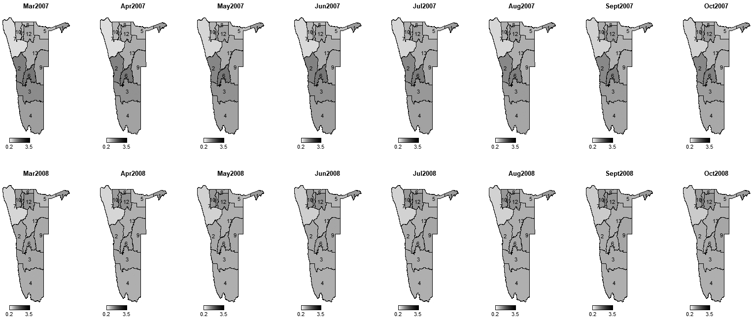
Figure 5.
Monthly incidence rate ratios of maintenance grant between 2009–2010.
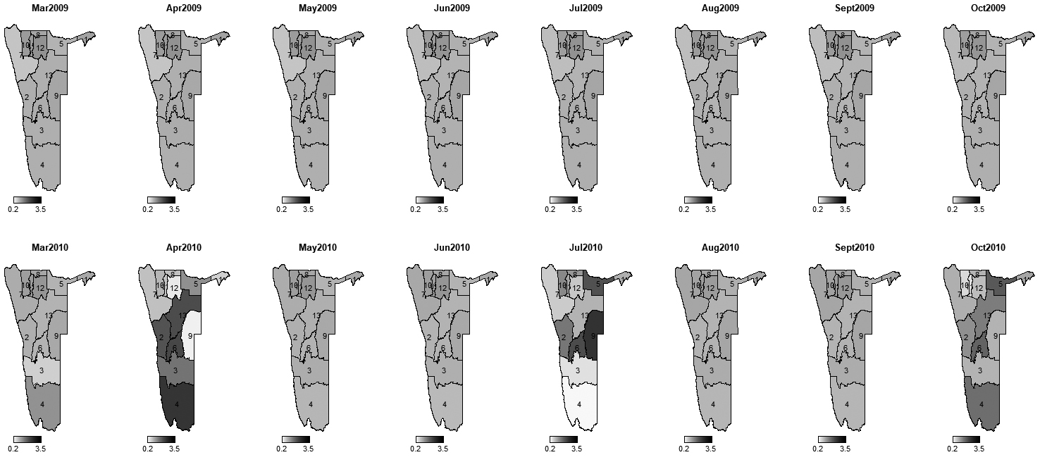
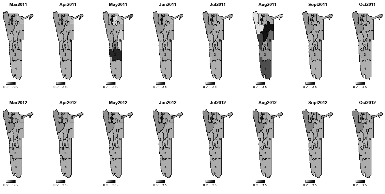
Figure 6.
Monthly incidence rate ratios of maintenance grant between 2011–2012.
The model with a larger value of
3.3Fixed and spatio-temporal effects
To quantify the relative influence of the neighborhood variables, we used the exponentiated fixed effects (
The adjustment of measurement error in orphanhood through the Berkson error model has not only ensured the stability of its effect, but also has considerably reduced the precision associated with structure spatial component (
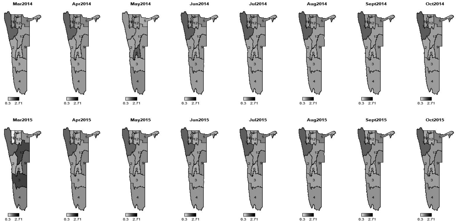
Figure 7.
Monthly incidence rate ratios of maintenance grant between 2013-2014
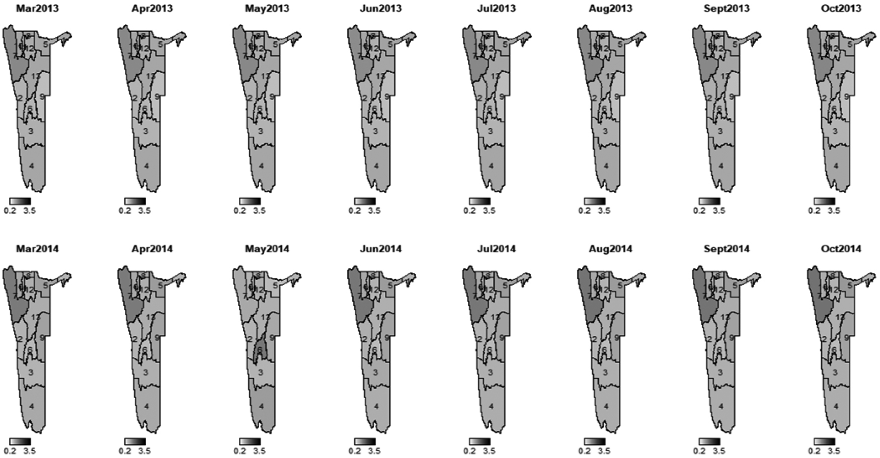
Figure 8.
Monthly incidence rate ratios of maintenance grant for 2015.
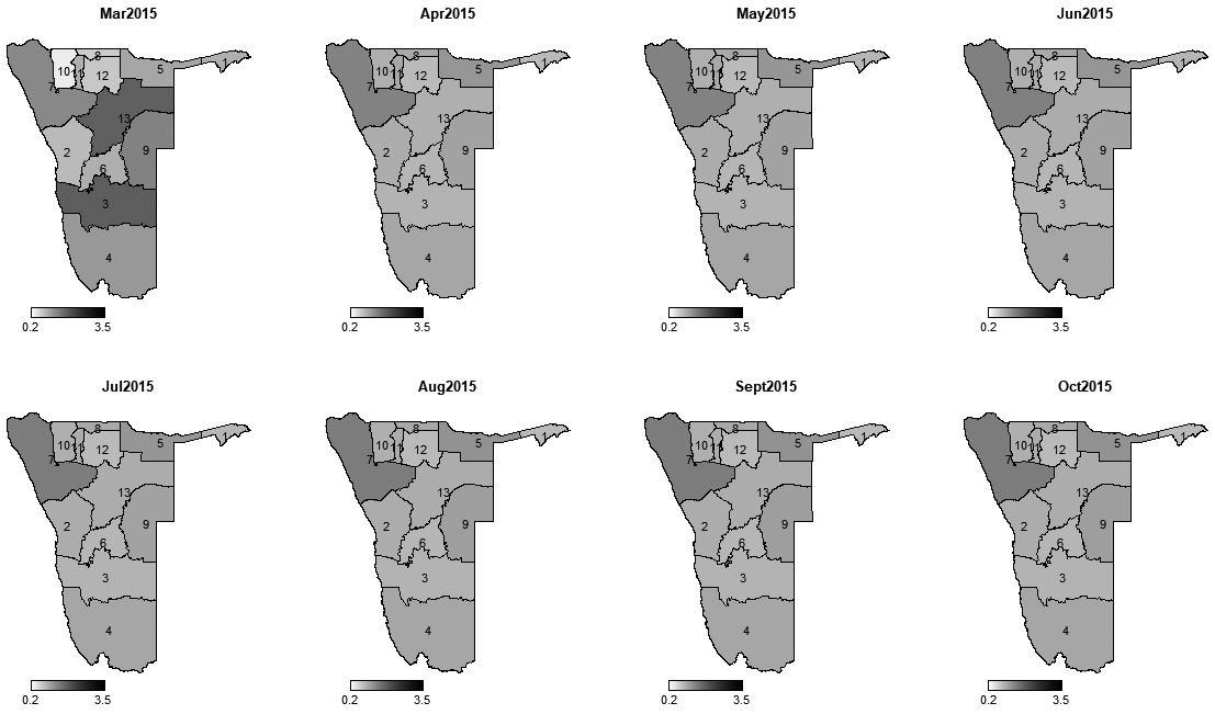
Figure 9.
Temporal paths of incidence rate ratios in regions for 2007–2015.
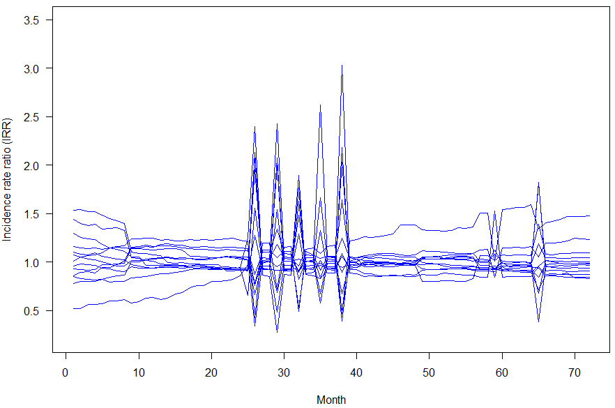
The introduction of spatial, temporal and spatio-temporal effects through Bayesian modelling approach allowed to quantify and map area-specific incidence rate ratio of child being on maintenance grant over the period of study. Thus, we were able to analyse incidence rate ratio differences among regions over the years. Figures 4–8 show the monthly incidence rate ratio for each region for a period of 9 years (2007–20015). From these maps, it can be noted that there exist variations in incidence rate ratio among regions during the study period. For example, Kunene region, which is labelled 7 had low incidence rate of maintenance grant during 2007–2010 but became a region with higher incidence as from 2011 to 2015. On the contrary, Erongo (labelled by 2) and Khomas (labelled by 6) had opposite trends to Kunene region as they were areas of grant high incidence rate ratio between 2007 and 2010 and became low incidence rate ratio areas from 2011 to 2015. Low rate ratio of maintenance grant were observed in Karas (labelled 3) and Hardap (labelled 4) regions throughout the study period. Figure 9 shows areas with increased or decreased child maintenance grant rate ratio over the years. This figure reveals that there were slight differences in rates of receiving grant among regions for the first 25 months and then suddenly spikes in risk were observed in the next 12 months, signaling remarkable differences in grant ratios, followed by a relative stability until 65th month.
Figure 10.
Maps of posterior probabilities of incidence rate ratios exceeding one for 2007–2008.
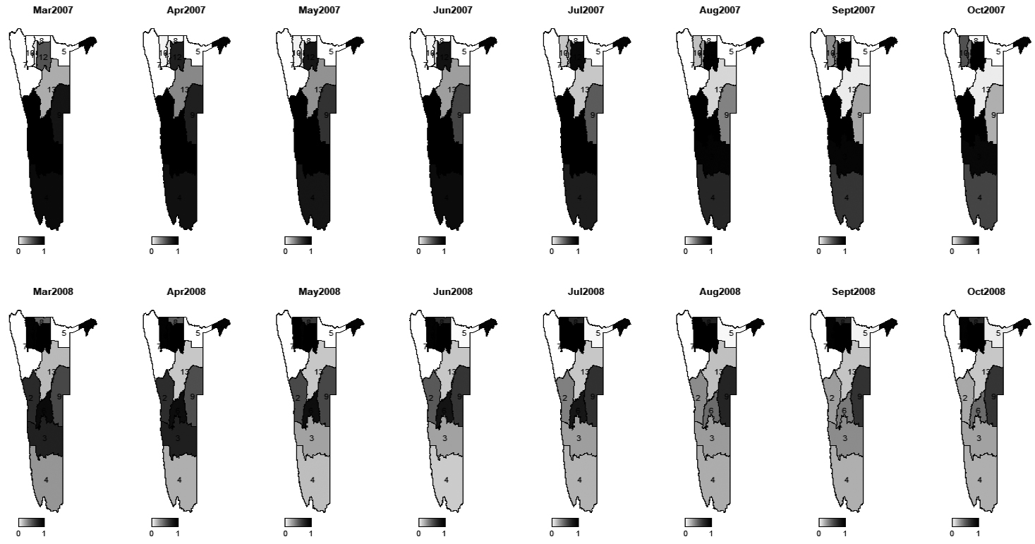
Figure 11.
Maps of posterior probabilities of incidence rate ratios exceeding one for 2009–2010.
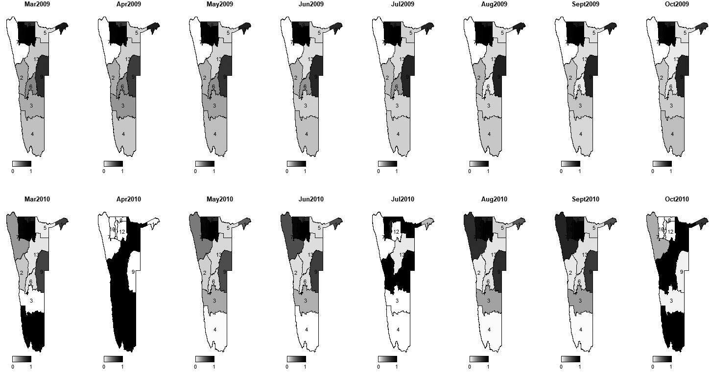
Figure 12.
Maps of posterior probabilities of incidence rate ratios exceeding one for 2011–2012.
Figure 13.
Maps of posterior probabilities of incidence rate ratios exceeding one for 2013–2014.
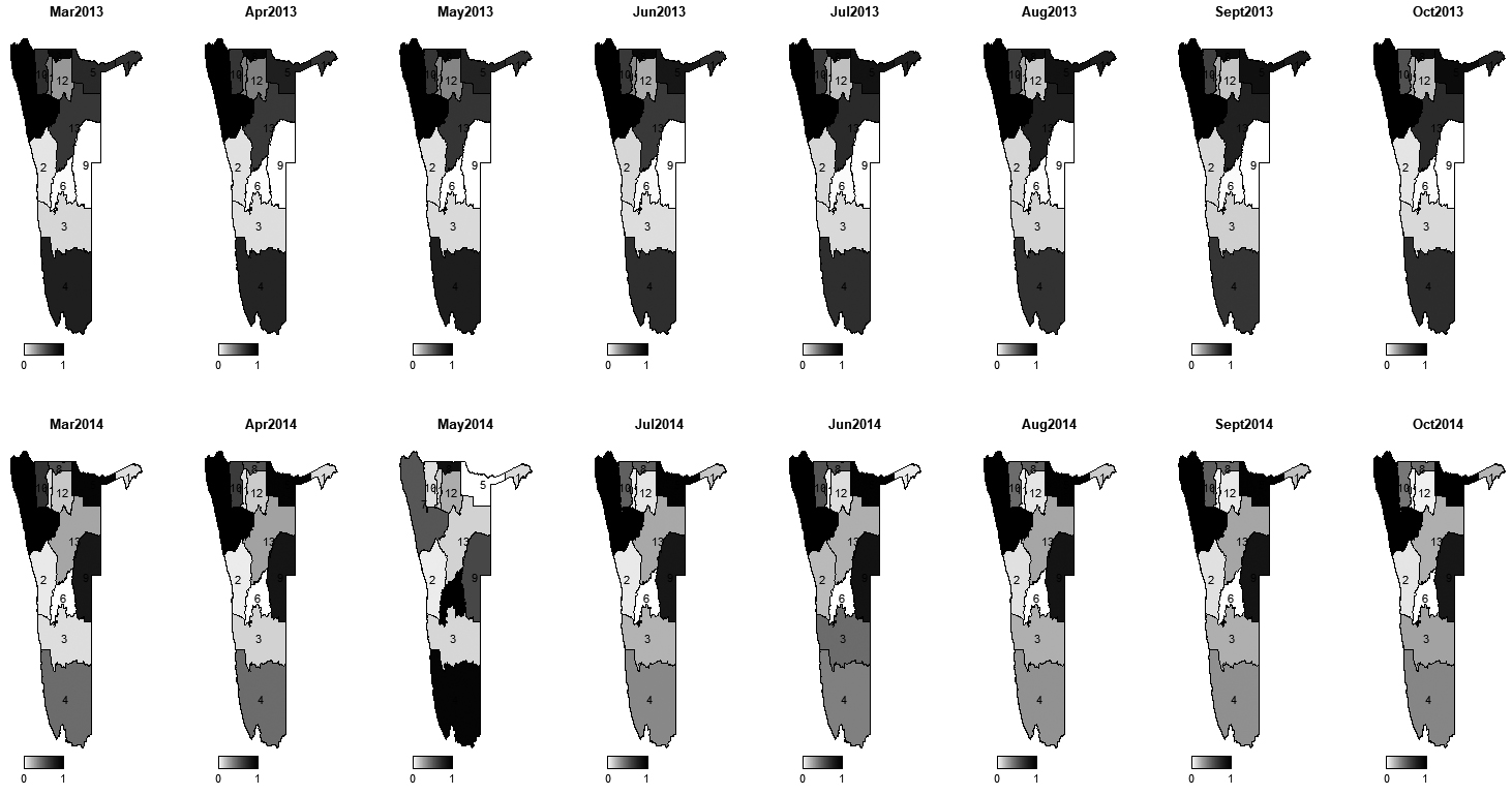
Figure 14.
Map of posterior probabilities of incidence rate ratios exceeding one for 2015.
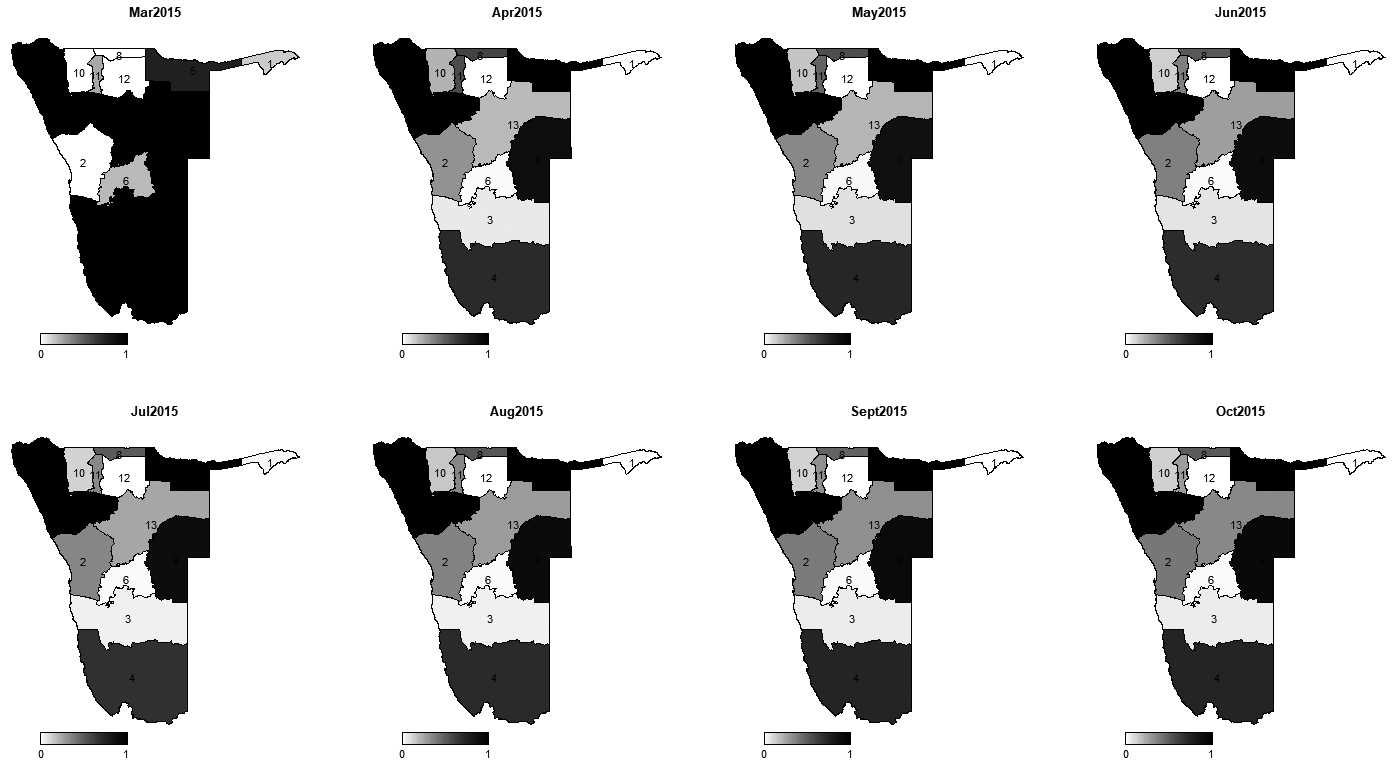
Like in disease mapping, the most important aspect of grant mapping is to determine the areas with excess incidence rate ratio of grant. To this effect, we mapped the probabilities of regions with incidence rate ratios exceeding one after adjusting for covariates and measurement errors (Figs 10–14). These maps reveal common patterns over the years, showing areas with higher levels of average number of children receiving the grant to be in the northern part of Namibia with exception of Oshikoto which was consistently at low risks except in 2007–2008 period. Also, it is worth noting that Caprivi region had high probability of incidence rate ratio exceeding one from 2007 to 2010 but its probability of incidence rate exceeding one gradually decreased close to zero.
Figure 15.
Posterior mean of the spatial effect (
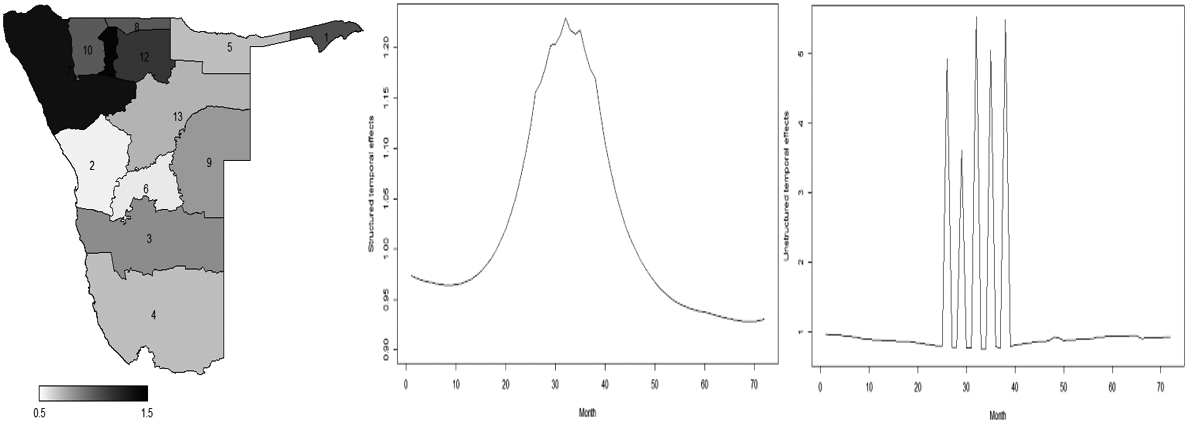
Figure 16.
Posterior mean of spatio-temporal interaction (
Common patterns of areas with lower levels of rate ratio in the southern part of Namibia (Hardap and Karas) were persistent over the years. Erongo region (in central east of Namibia) and Omaheke (in central west of Namibia) had higher maintenance rate ratio, while the regions in central Namibia that include Khomas and Otjozondjupa had moderate probabilities to be classified as areas in need of maintenance grant.
After accounting for variability of grant distribution due to covariates (unemployment and orphanhood), it is crucial to examine how much variation is still unexplained. Figures 15 and 16 show the spatial, temporal, and spatio-temporal effects. These effects are interpreted as residuals after accounting for covariates. Figure 15 (left panel) reveals that high residuals, unexplained variation after accounting for effect of covariates, were in Kunene (labelled 7) and Oshana (labelled 11) regions. Zambezi (1) and Oshikoto (12) regions had moderate residuals whereas the rest of Namibia had low residuals.
A bell shape trend of structured effects is visible across years with an average effect located approximately in the 35
4.Discussion and conclusions
In this study Bayesian spatio-temporal models were fitted to assess the regional patterns and trends of maintenance grants in Namibia. Findings of this study showed strong regional differences in incidence rate ratios of maintenance grant. Regions with higher levels of average number of children receiving the grant were found in the northern part of Namibia apart from Oshikoto which consistently showed low levels of incidence rate ratio. Statistically significant fluctuations in child maintenance grant distribution were observed over the study period, particularly between March 2010 and August 2011.
The temporal analysis revealed that Kunene had gradually become a pocket of higher incidence rate ratio of maintenance grant Between 2007 and 2009, the number of children on maintenance grant was relatively low and became significantly high between 2010 and 2015. An opposite temporal trend was observed in Zambezi region, which had elevated number of children on grant between 2007 and 2013 and suddenly the incidence rate ratio of the grant decreased significantly in 2014 and 2015. As the levels of unemployment had increased over the study period in both regions, one would naturally expect to see an increase in number of children getting the maintenance grant. However, in the latter province, the temporal trend showed otherwise.
Additionally, our results showed that regions with high levels of unemployment and orphanhood had higher average of number of children under maintenance grant. This finding stresses the importance of the covariates on maintenance grant distribution. Also, this finding agrees with the finding of the study by [39], which established the relationship between orphanhood and fostering.
The knowledge of spatial and temporal patterns is essential in providing the insight on the relationship between regional grant distribution and characteristics of a region, and hence to identifying incidence rate ratio hot spots. Thus, the findings from this study will be useful in developing a more refined targeted intervention model for grant distribution in Namibia.
One of the limitations of this study is that only two covariates were used to explain the variations in grant distribution and in addition those variables were not available for each year of the study period. For example, in this study socioeconomic covariates such as education of caregivers and levels of motivation of caregivers, which were found to be statistically associated with grant seeking behavior [40], were not available. This could have an impact on parameter estimates. However, the use of the Bayesian spatio-temporal modelling approach [34] and the adjustment of measurement error in covariates through Berkson model mighty have lessened the abnormality [41].
Another limitation to this study includes the type of neighbourhood units used, namely, region is also a potential limitation as the smallest geographical administrative unit such as a constituency would have been ideal to ensure the high-resolution approach and particularly adequately capture neighborhood influences on small area variations in incidence rate ratio. However, the use of regions as neighbourhood units was dictated by the available data. Analysing this type of data at lower levels would have introduced another problem known as misalignment [42].
In conclusion, this study has shown the strength of using spatial-temporal statistical methods coupled with measurement error models for analysing child grant data and is one of the few studies to have used Bayesian spatio-temporal modelling approach on maintenance grant data. Furthermore, the study has demonstrated that the northern regions of Namibia have the highest child incidence rate ratio of maintenance grant whereas the regions in central and south are at low incidence rate at present. Additionally, the maps produced in this study can be particularly helpful in allocating efficiently limited resources in poor settings through identification of regions with high incidence rate of child maintenance grant.
Furthermore, they will assist the policymakers in planning and developing targeted intervention intended to reduce unemployment and orphanhood in northern part of Namibia as both the unemployment and orphanhood were significant risk factors of spatio-temporal child maintenance grant distribution.
Acknowledgments
We thank the Ministry of Gender Equality and Child Welfare for providing the dataset used in this study.
Conflict of interest
On behalf of all authors, the corresponding author states that there is no conflict of interest.
References
[1] | Niño-Zarazúa M, Barrientos A, Hickey S, Hulme D. Social protection in Sub-Saharan Africa: Getting the politics right. World Development. (2012) ; 40: (1): 163-176. |
[2] | Samad SA. Empowering Social Protection System. The Role of Government and a Way Forward. Journal of Administrative Science. (2019) ; 16: (2): 27-41. |
[3] | Dinbabo MF. Social welfare policies and child poverty in South Africa: a microsimulation model on the Child Support Grant (Doctoral dissertation, University of the Western Cape, 2011). |
[4] | Borges FA. Adoption and Evolution of Cash Transfer Programs in Latin America. InOxford Research Encyclopedia of Politics (2019) Oct 30. |
[5] | Stover J, Bollinger L, Walker N, Monasch R. Resource needs to support orphans and vulnerable children in sub-Saharan Africa. Health Policy and Planning. (2007) Jan 1; 22: (1): 21-7. |
[6] | Bamfo NA. Child beggars and vendors on city streets in Sub-Saharan Africa visible, bold, and neglected. Africa Insight. (2018) Dec 1; 48: (3): 33-58. |
[7] | Devereux S. Social protection for enhanced food security in sub-Saharan Africa. Food policy. (2016) Apr 1; 60: : 52-62. |
[8] | Hansen J, Hellin J, Rosenstock T, Fisher E, Cairns J, Stirling C, Lamanna C, van Etten J, Rose A, Campbell B. Climate risk management and rural poverty reduction. Agricultural Systems. (2019) Jun 1; 172: : 28-46. |
[9] | Carter DJ, Glaziou P, Lönnroth K, Siroka A, Floyd K, Weil D, Raviglione M, Houben RM, Boccia D. The impact of social protection and poverty elimination on global tuberculosis incidence: a statistical modelling analysis of Sustainable Development Goal 1. The Lancet Global Health. (2018) May 1; 6: (5): e514-22. |
[10] | Kidd S. Social protection: an effective and sustainable investment in developing countries. (2014) ; doi: 10.13140/2.1.4878.3683. |
[11] | Kaplan J, Jones N. Child-sensitive social protection in Africa: challenges and opportunities. Addis Ababa: ACPF and ODI. (2013) . |
[12] | Bright T, Felix L, Kuper H, Polack S. A systematic review of strategies to increase access to health services among children in low and middle income countries. BMC Health Services Research. (2017) Dec 1; 17: (1): 252. |
[13] | Grinspun A. No small change: The multiple impacts of the Child Support Grant on child and adolescent well-being. ChildGauge. (2016) : 44. |
[14] | Ferrando M. Cash transfers and school outcomes: the case of Uruguay. Master’s thesis, Université Catholique de Louvain, Louvain-la-Neuve, Belgium. (2012) . |
[15] | Kaldal A, Landberg Å, Eriksson M, Svedin CG. Children’s right to information in Barnahus. InCollaborating Against Child Abuse (2017) ; (pp. 207-226). Palgrave Macmillan, Cham. |
[16] | Sulla V, Zikhali P, Schuler PM, Jellema JR. Does fiscal policy benefit the poor and reduce inequality in Namibia? The World Bank; (2017) Jun 1. |
[17] | Chiripanhura B, Niño-Zarazúa M. Social safety nets in Namibia: Structure, effectiveness and the possibility for a universal cash transfer scheme. The Basic Income Grant as Social Safety Net for Namibia: Experience and lessons from around the world. (2013) Sep 26: : 13. |
[18] | Ministry of Gender, Equality and Child Welfare. The Effectiveness of Child Welfare Grants in Namibia (2010). |
[19] | Schade K, La J, Pick A. Financing social protection in Namibia (2019). |
[20] | Stewart D, Okubo T. A World Free from Child Poverty, (2017) . |
[21] | Kgawane-Swathe TE. Examining the contribution of child support grant towards the alleviation of poverty: a case of South African Social Security Agency, Masodi Village, Limpopo Province, South Africa (Doctoral dissertation, 2014). |
[22] | Tjivikua KK, Olivier M, Likukela M. Institutional Assessment of Namibia’s Social Protection System: Strengths, Weaknesses, future challenges and reforming options for the governance of the social protection system in Namibia (2018). https//thl.fi/documents/189940/2152174/SPSIA_Namibia_Final+Report-+20180112.pdf/126584f9-0452-44e3-a40b-27c83c7f5352 (accessed 6 May 2020). |
[23] | International Labour Organization (2014). Namibia Social Protection Floor Assessment. (2014) , Htt//www.ilo.org/publns. Accessed 6 May 2020. |
[24] | Manda SO, Kandala NB, Ghilagaber G. Advanced techniques for modelling maternal and child health in Africa. InAdvanced Techniques for Modelling Maternal and Child Health in Africa (2014) ; (pp. 1-7). Springer, Dordrecht. |
[25] | Tlou B, Sartorius B, Tanser F. Spatial-temporal dynamics and structural determinants of child and maternal mortality in a rural, high HIV burdened South African population, 2000–2014: a study protocol. BMJ Open. (2016) Jul 1; 6: (7): e010013. |
[26] | Sartorius B, Kahn K, Collinson MA, Vounatsou P, Tollman SM. Survived infancy but still vulnerable: spatial-temporal trends and risk factors for child mortality in rural South Africa (Agincourt), 1992–2007. Geospatial Health. (2011) May; 5: (2): 285. |
[27] | Gracia E, López-Quílez A, Marco M, Lila M. Mapping child maltreatment risk: A 12-year spatio-temporal analysis of neighborhood influences. International Journal of Health Geographics. (2017) Dec 1; 16: (1): 38. |
[28] | Dunson DB. Commentary: practical advantages of Bayesian analysis of epidemiologic data. American Journal of Epidemiology. (2001) Jun 15; 153: (12): 1222-6. |
[29] | Greenland S. Bayesian perspectives for epidemiological research: I. Foundations and basic methods. International Journal of Epidemiology. (2006) Jun 1; 35: (3): 765-75. |
[30] | Bryant JR, Graham P. A Bayesian approach to population estimation with administrative data. Journal of Official Statistics. (2015) Sep 1; 31: (3): 475-87. |
[31] | Bijak J, Bryant J. Bayesian demography 250 years after Bayes. Population Studies. (2016) Jan 2; 70: (1): 1-9. |
[32] | Gelman A, Shalizi CR. Philosophy and the practice of Bayesian statistics. British Journal of Mathematical and Statistical Psychology. (2013) Feb; 66: (1): 8-38. |
[33] | Lynch SM, Bartlett B. Bayesian Statistics in Sociology: Past, Present, and Future. Annual Review of Sociology. (2019) Jul 30; 45: : 47-68. |
[34] | Blangiardo M, Cameletti M. Spatial and spatio-temporal Bayesian models with R-INLA. John Wiley & Sons; (2015) Jun 2. |
[35] | Besag J, York J, Mollié A. Bayesian image restoration, with two applications in spatial statistics. Annals of the Institute of Statistical Mathematics. (1991) Mar 1; 43: (1): 1-20. |
[36] | Martínez-Beneito MA, López-Quilez A, Botella-Rocamora P. An autoregressive approach to spatio-temporal disease mapping. Statistics in Medicine. (2008) Jul 10; 27: (15): 2874-89. |
[37] | Knorr-Held L. Bayesian modelling of inseparable space-time variation in disease risk. Statistics in Medicine. (2000) Sep 15; 19: (17-18): 2555-67. |
[38] | Ntirampeba D, Neema I, Kazembe L. Modelling spatio-temporal patterns of disease for spatially misaligned data: An application on measles incidence data in Namibia from 2005-2014. PloS One. (2018) Aug 13; 13: (8): e0201700. |
[39] | Grant MJ, Yeatman S. The relationship between orphanhood and child fostering in sub-Saharan Africa, 1990s–2000s. Population Studies. (2012) Nov 1; 66: (3): 279-95. |
[40] | Coetzee M. Do poor children really benefit from the child support grant. |
[41] | Buonaccorsi JP. Measurement error: models, methods, and applications. CRC press; (2010) Mar 2. |
[42] | Banerjee S, Carlin BP, Gelfand AE. Hierarchical modeling and analysis for spatial data. CRC press; (2014) Sep 12. |


