
Model-based estimation of small area food insecurity measures in Ethiopia using the Fay-Herriot EBLUP estimator
Abstract
In many countries, including Ethiopia, sample surveys are designed to produce estimates of variables of interest at the national and regional levels due to cost and operational considerations. For example, household food insecurity estimates are needed down at least at the zone level in Ethiopia to offer targeted solutions. However, the sample sizes of sample surveys are often not large enough to produce reliable estimates at the small area (zone) level. This paper remedies some of these shortcomings by estimating household food insecurity in each zone of Ethiopia by linking data from the 2015/16 welfare and monitoring survey and the 2007 population census using a small area estimation (SAE) approach. The results show the zonal level household food insecurity estimates generated by SAE were more efficient and precise compared to the survey-based estimates. Besides, accurate and cost-effective food insecurity statistics at the zonal level were produced without more resources through combining the available data sources. Finally, zonal level household food insecurity estimates could be the recommended tools for monitoring the progress of sustainable development goals (SDGs) in Ethiopia. Because, in the final 2030 Agenda, SDG 2 concentrates entirely on food security, recognizing much of its complex and multi-faceted nature.
1.Introduction
Food insecurity refers to a lack of food due to lack of resources, not because of illness or voluntary fasting or dieting. It is the state of being without regular access to nutritious and sufficient amounts of food for active and healthy life including normal growth and development [1, 2]. Having low monthly income, large household size, low educational level, unemployment among adult members, single female head, inadequate dietary intake, and poor nutritional status are the most common variables related to food insecurity at the household level [3]. In other words, food insecurity is to a large extent related to low socio-economic status.
Based on the latest FAO estimates, about 1.3 billion people in the world consisting of 17.2% of the world population have experienced food insecurity at moderate levels [2]. About 2 billion people in the world consisting of 26.4% of the world population have experienced a combination of moderate and severe levels of food insecurity [2]. Among those affected, the majority live in sub-Saharan Africa (SSA) (22.8%), Southern Asia (15.0%) and Western Asia (12%). The undernourished population is distributed unevenly across regions. For example, in 2018 more than 500 million in Asia and almost 260 million people in Africa are undernourished with 90% living in SSA [2].
Currently, food insecurity and its alleviation are one of the international community’s main priorities, especially in SSA [4, 5]. According to the latest estimates of the State of Food Insecurity in the World [6], the prevalence of hunger for SSA declined by 31% between 1990 and 2015. Although the prevalence of hunger declined from 75% to 32% in Ethiopia, approximately 26 million people were categorized as food insecure in 2016 [7, 8]. During this period, however, the number of hungry people fell from 37 to 32 million [9].
Ethiopia is among the countries affected by food shortages since the 1960s [10]. The country has faced three different famines in the past four decades [7, 9]. Consequently, the famines in the 1970s, 80s, and 90s affected much of the country’s subsequent food production. It was estimated that close to 58 million people were affected by famine between 1973 and 1986 [11]. However, food insecurity continues to be a challenge to the Ethiopian Government despite the country coming a long way in reducing it [7]. Food insecurity patterns of Ethiopia are linked with rainfall patterns, where hunger trends decline after the rainy seasons [12]. Poverty and hunger were found to be the highest in the rural areas where the majority of the poor live [9].
Ethiopia is among the countries that have achieved the millennium development goals (MDGs) target between 1990 and 2015 [6]. For example, Ethiopia has made progress in reducing food insecurity and malnutrition [13], especially the prevalence of undernourishment reduced from the 60% level seen in the 1990s to 30% in 2015 [14, 15]. However, the country has experienced one of the worst droughts in half a century due to the La Niña effect in 2015 [16]. The La Niña effect resulted in low summer rainfall in all parts of the country [16], which is often led the country with food security crises [17]. As a result of the drought, many farmers, herders, and families dependent on agriculture have been forced to migrate and become dependent on humanitarian assistance to rescue themselves from widespread hunger and malnutrition [18].
Given that Ethiopia has experienced high scale famine with the potential for recurrence, it is important to provide adequate information for the Government, stakeholders, policymakers and Nongovernmental Organizations (NGOs) for necessary interventions. This paper aims at contributing to two aspects including:-
• First, food insecurity measures are understudied in the literature compared with poverty, especially in developing countries. This paper presents a set of estimates of food insecurity measures in Ethiopia, underpinned by a method that does not receive much attention in food security literature.
• Second, official estimates of poverty, food insecurity, and so on in Ethiopia are available at the national and regional levels. However, there is a need for geographically disaggregated estimates at the sub-national levels (i.e., zones and regional towns) for making better decisions. The national government, as well as zonal level administrative officials, would like to know how they can prioritize and allocate resources. Because zonal level estimates could be used as a basis for identifying marginalized households and communities to ensure the equitable and inclusive provision of assistance to the ones most in need. Furthermore, zonal level estimates are needed to adequately allocate funds and to be able to assess the effectiveness of their spending [19].
Having this in mind, the aim of this paper is twofold. First, the primary aim is to account for inequality in food insecurity measures at the zone levels in Ethiopia. Second, this paper analyses geographical (spatial) variations of food insecurity measure at the zone levels in Ethiopia.
2.Materials and methods
2.1The study area
Ethiopia is located in eastern Africa, bordered by Sudan and South Sudan to the west, Kenya to the south, Eritrea to the north, Djibouti to the east and Somalia to the south and east. The GPS coordinates of Ethiopia is 9.1450
2.2Data sources
Small area estimation depends on a combination of different datasets such as survey data and census data [19]. The welfare and monitoring survey (WMS) was conducted by the government statistical agency, Central Statistical Authority (CSA) in 2015/16 [21]. The survey covered the population in sedentary areas of the country on a sample basis excluding the non-sedentary population in Afar and Somali Regions. The sampling method considered under this category was a stratified multi-stage cluster sampling with enumeration areas as the second-stage sampling units. In summary, a total of 30,237 households (10,368 in rural and 19,869 in urban areas) were covered. To fill the possible gap in the survey data we used the auxiliary information from the 2007 Ethiopian population census data.
2.3The Fay-Herriot model and small-area estimators
In particular, since food insecurity measures depend on the binary outcome from the question (“Did the household suffer food shortage during the last 12 months?”), neither linear mixed models nor unit-level model-based estimation approaches can hardly be used [22]. Instead, the Fay-Herriot model gives an easy-to-apply solution [22]. Therefore, the well-known Fay-Herriot model is applied to obtain estimates of food insecurity measures at the zone levels in Ethiopia. This model is useful in cases where auxiliary data are available at the area level or when it is not possible to link the information of the sample units with census data or unit-level data, which might not be available due to confidentiality issues [23, 24].
Following [24], the model is described as: let
(1)
denote the
(2)
The Fay-Herriot model is therefore expressed as:
(3)
where the area specific random effects
2.4Empirical best linear unbiased predictor (EBLUP) estimator
Small area means or totals can be expressed as linear combinations of fixed and random effects. The best known method for the prediction of mixed effects is the best linear unbiased predictor (BLUP). The BLUP estimator was first originated by [25] and used by many authors in different applications. It is a weighted combination of the direct estimator,
(4)
where
Since
(5)
where
(6)
The equation is iteratively solved subject to the condition
(7)
where
When the variance of the area effect,
(8)
where
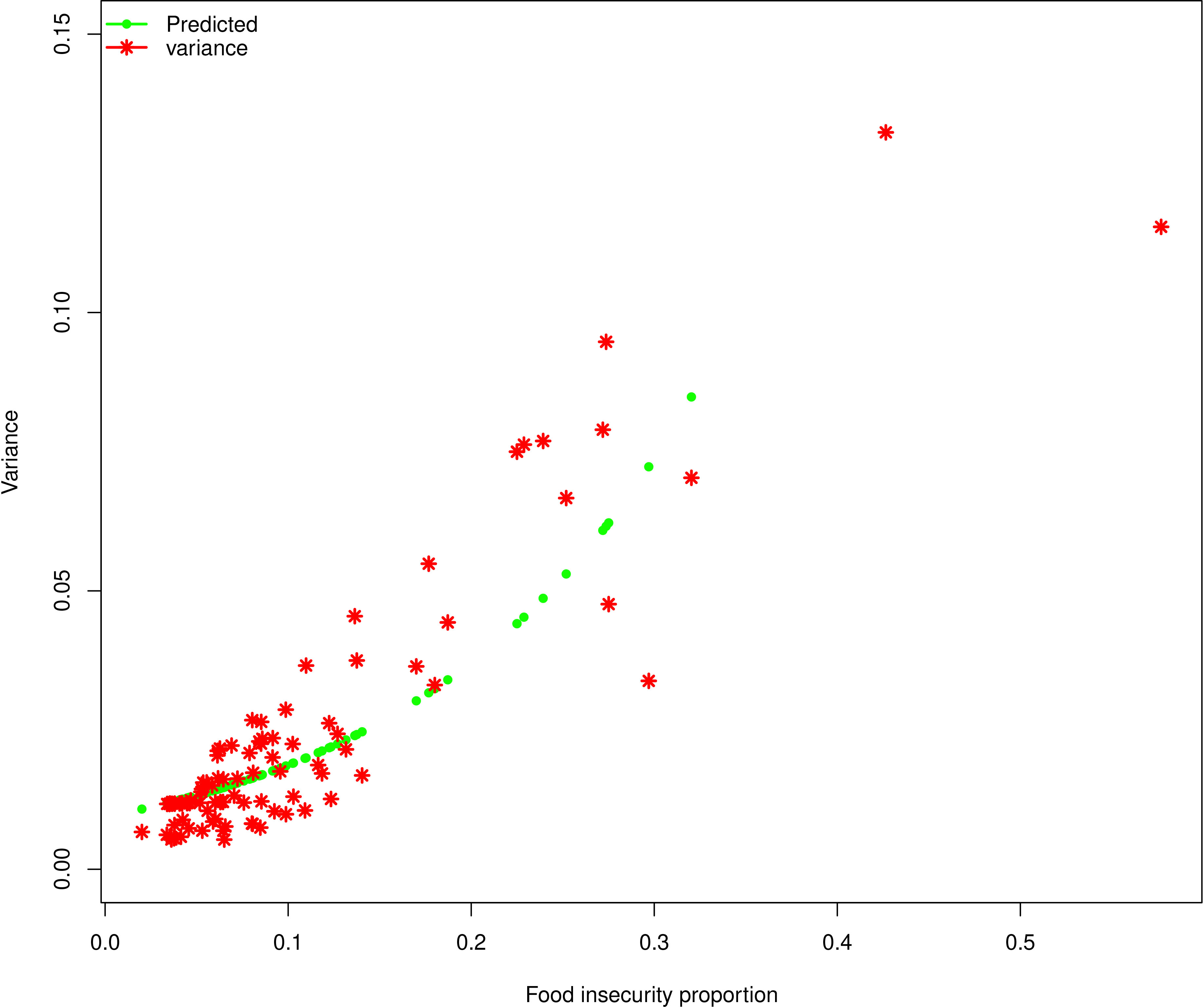
Figure 1.
Dispersion plots for GVF fit for food insecurity estimates.
2.5Estimation of MSE of EBLUP
In practical applications, we need an estimator of
(9)
where
This estimator accounts for the variability (or uncertainty) associated with the estimation of the regression parameters, random effects, and variance components. According to [30], the
A nearly unbiased estimator of
(10)
where
Let
(11)
Let
The Akaike information criterion (AIC), Bayesian information criterion (BIC) and log-likelihood function were used to select the auxiliary variables [26]. In general, a desirable model is one that minimizes the AIC or the BIC on the significance tests for each parameter. The model was operationalized using the R statistical software package. Furthermore, the steps and procedures required to obtain small area estimates are discussed by [31].
Furthermore, the generalized variance function (GVF) introduced by [24] was applied to smooth out the uncertainty of the design-based variance estimate in a complex setting. When sample sizes are too small, standard design-based estimators are not precise enough. It is important to have stable estimators for smaller domains. The GVF is used to produce domain-level variance estimators that would be more stable than direct design-based variance estimators. As shown in Fig. 1, the GVF helps to smooth out the unreliable and noisy estimated variance [22].
Table 1
Estimates of the log-transformed FH model parameters
| Estimate | Std error | ||||
|---|---|---|---|---|---|
| Women |
| 3.695 | 1.046 | 3.532 | 0.001 |
| Age less than or equal to 30 |
| 0.515 | 0.608 | 0.847 | 0.399 |
| Single |
| 0.062 | 0.161 | 0.387 | 0.699 |
| Greater than 12 years of schooling |
| 0.065 | 0.005 | ||
| Self employed |
| 0.319 | 0.123 | 2.589 | 0.011 |
| Household size less than 5 |
| 0.514 | 0.175 | ||
| Adjusted r-square | 0.95 | ||||
| AIC | 174.35 | ||||
| BIC | 191.93 | ||||
| Loglik | | ||||
Note: *significant at 0.05 and **significant at 0.01.
3.Results and discussion
In the usual application of standard small area estimation, data on the variables of interest would be taken from the survey while data on the auxiliary variables would be taken from the census data [26]. The estimated proportion of food-insecure households in Ethiopian zones calculated from the 2015/16 WMS data acts as the response variable in the Fay-Herriot regression model. As auxiliary (i.e., explanatory) variables, we considered the indicators of age, the indicators of sex, the indicators of the different levels of the variable education, the indicators of the categories of the variable employment, indicators of marital status and indicators of household size.
Table 1 reports the estimates of the Fay-Herriot model parameters and the corresponding
Figure 2.
The EBLUPs and direct estimates for each zone.
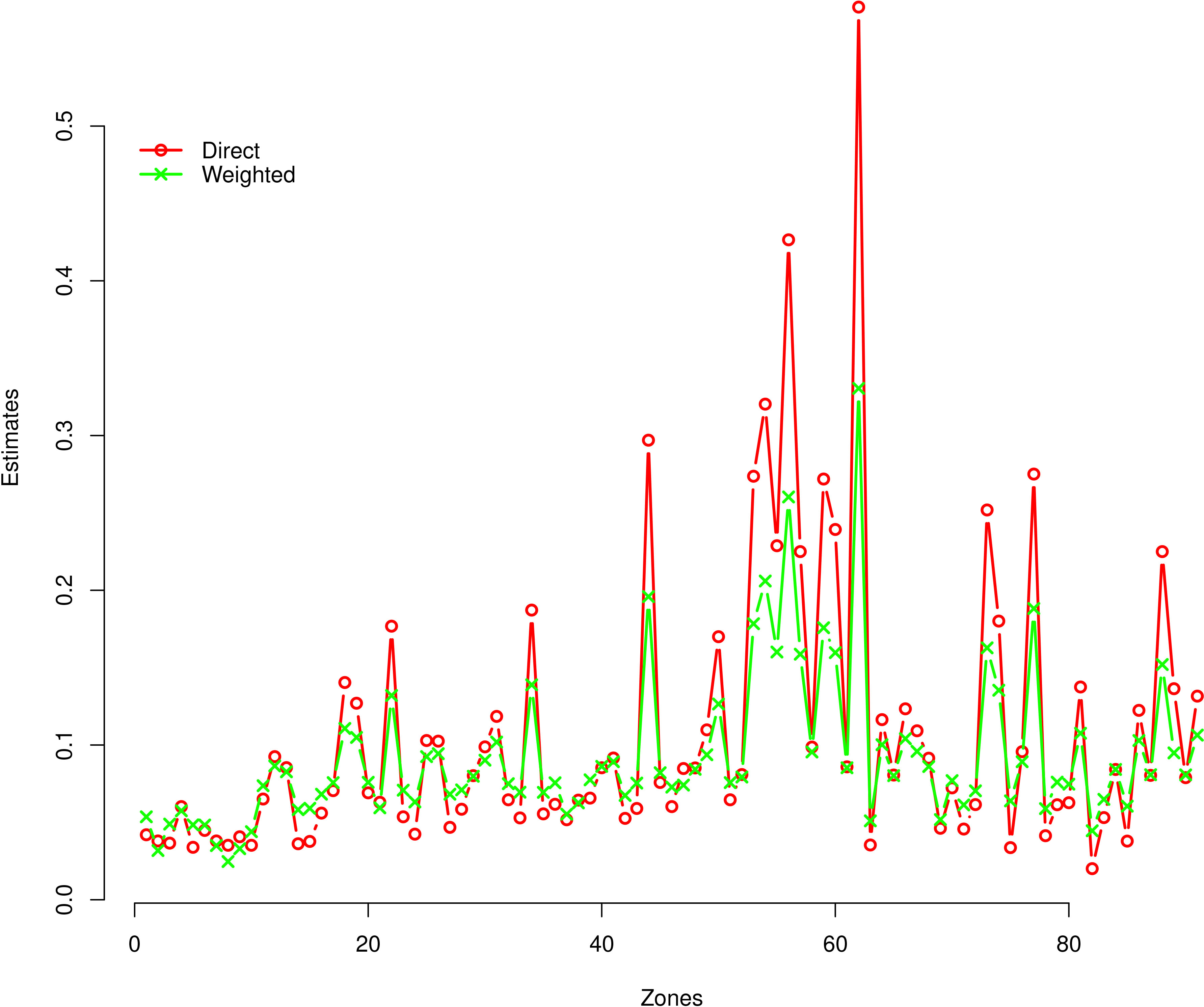
The estimation results for all the zones are shown in Table 2. The smallest zonal level food insecurity estimates (
Figure 3.
Plot illustrating the RMSEs (left) and CVs (right) of household food insecurity along the Ethiopian zones in 2015/16.
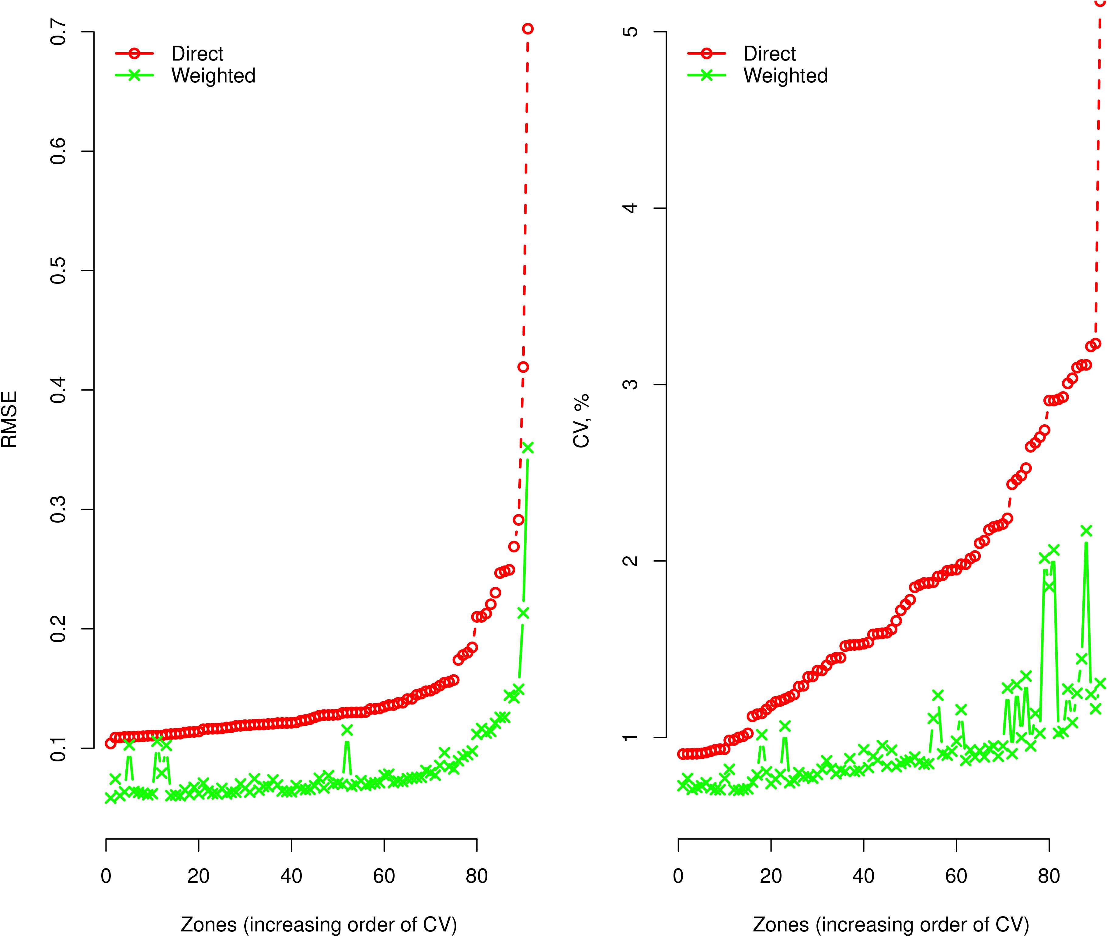
Table 2
Estimates of household food insecurity for the Ethiopian zones. RMSE is the root mean squared error of the estimates. CV is the coefficient of variation of the estimates
| Zones | Weighted (%) |
|
|
|
|
|---|---|---|---|---|---|
| Akaki | 5.36 | 0.0609 | 0.1121 | 1.1363 | 2.6694 |
| Nifas Silk | 3.18 | 0.1059 | 0.1106 | 1.8547 | 2.9093 |
| Kolfe | 4.89 | 0.0623 | 0.1100 | 1.2738 | 3.0065 |
| Gulele | 5.75 | 0.0665 | 0.1193 | 1.1570 | 1.9818 |
| Lideta | 4.84 | 0.0603 | 0.1090 | 1.2441 | 3.2160 |
| Kirkos | 4.83 | 0.0651 | 0.1132 | 1.3476 | 2.5262 |
| Arada | 3.50 | 0.0792 | 0.1106 | 2.0629 | 2.9093 |
| Addis Ketema | 2.47 | 0.1028 | 0.1095 | 2.1715 | 3.1116 |
| Bole | 3.30 | 0.1024 | 0.1116 | 2.0165 | 2.7418 |
| Yeka | 4.40 | 0.0635 | 0.1095 | 1.4453 | 3.1106 |
| North Gondar | 7.37 | 0.0635 | 0.1213 | 0.8614 | 1.8636 |
| South Gondar | 8.65 | 0.0712 | 0.1333 | 0.8228 | 1.4410 |
| North Wollo | 8.27 | 0.0728 | 0.1301 | 0.8798 | 1.5232 |
| South Wollo | 5.82 | 0.0630 | 0.1099 | 1.0837 | 3.0358 |
| Norths Shewa | 5.91 | 0.0611 | 0.1104 | 1.0336 | 2.9293 |
| East Gojam | 6.82 | 0.0630 | 0.1176 | 0.9247 | 2.1003 |
| West Gojam | 7.57 | 0.0653 | 0.1236 | 0.8628 | 1.7532 |
| Waghmra | 11.07 | 0.0827 | 0.1571 | 0.7466 | 1.1192 |
| Awi | 10.49 | 0.0775 | 0.1501 | 0.7384 | 1.1816 |
| Oromo Zone | 7.59 | 0.0660 | 0.1230 | 0.8700 | 1.7805 |
| Bahirdar | 5.94 | 0.0735 | 0.1205 | 1.2390 | 1.9122 |
| Argoba | 13.20 | 0.0931 | 0.1780 | 0.7055 | 1.0069 |
| West Wollega | 7.08 | 0.0664 | 0.1167 | 0.9378 | 2.1765 |
| East Wollega | 6.32 | 0.0602 | 0.1123 | 0.9520 | 2.6474 |
| Illubabor | 9.25 | 0.0721 | 0.1381 | 0.7797 | 1.3425 |
| Jimma | 9.44 | 0.0725 | 0.1380 | 0.7689 | 1.3459 |
| West Shewa | 6.82 | 0.0618 | 0.1139 | 0.9072 | 2.4347 |
| North Shewa | 7.10 | 0.0632 | 0.1186 | 0.8892 | 2.028 |
| East Shewa | 7.98 | 0.0668 | 0.1278 | 0.8365 | 1.5935 |
| Arsi | 9.02 | 0.0712 | 0.1362 | 0.7897 | 1.3786 |
| West Harerge | 10.19 | 0.0757 | 0.1458 | 0.7431 | 1.2301 |
| East Harerge | 7.50 | 0.0638 | 0.1211 | 0.8508 | 1.8753 |
| Bale | 6.95 | 0.0621 | 0.1164 | 0.8933 | 2.1996 |
| Borena | 13.89 | 0.0977 | 0.1845 | 0.7033 | 0.9854 |
| South West Shewa | 6.94 | 0.0618 | 0.1174 | 0.8897 | 2.1152 |
| Guji | 7.56 | 0.0680 | 0.1199 | 0.8993 | 1.9439 |
| Adama | 5.53 | 0.0708 | 0.1159 | 1.2798 | 2.2417 |
| Jimma Liyu | 6.26 | 0.0693 | 0.1211 | 1.1077 | 1.8798 |
| West Arsi | 7.75 | 0.0688 | 0.1216 | 0.8886 | 1.8507 |
| Kellem Wollega | 8.62 | 0.0696 | 0.1300 | 0.8071 | 1.5246 |
| Horogudru | 8.92 | 0.0709 | 0.1329 | 0.7942 | 1.4509 |
| Gurage | 6.74 | 0.0641 | 0.1162 | 0.9513 | 2.2096 |
| Hadya | 7.54 | 0.0701 | 0.1188 | 0.9290 | 2.0140 |
| Kembata | 19.59 | 0.1423 | 0.2689 | 0.7261 | 0.9053 |
| Sidama | 8.21 | 0.0685 | 0.1259 | 0.8344 | 1.6607 |
| Gedeo | 7.28 | 0.0633 | 0.1193 | 0.8692 | 1.9819 |
| Wolayita | 7.41 | 0.1153 | 0.1298 | 0.9307 | 1.5309 |
| South Omo | 8.43 | 0.0684 | 0.1300 | 0.8118 | 1.5259 |
| Sheka | 9.37 | 0.0750 | 0.1414 | 0.8002 | 1.2881 |
| Kefa | 12.65 | 0.0896 | 0.1739 | 0.7084 | 1.0231 |
| Gamo Gofa | 7.57 | 0.0642 | 0.1211 | 0.8487 | 1.8749 |
| Benci Maji | 7.93 | 0.0708 | 0.1281 | 0.8923 | 1.5836 |
| Yem | 17.84 | 0.1259 | 0.2482 | 0.7054 | 0.9068 |
| Amaro | 20.60 | 0.1494 | 0.2913 | 0.7253 | 0.9093 |
| Burji | 16.01 | 0.1128 | 0.2128 | 0.7041 | 0.9300 |
| Konso | 26.03 | 0.2133 | 0.4192 | 0.8192 | 0.9830 |
| Derashe | 15.87 | 0.1116 | 0.2100 | 0.7032 | 0.9334 |
| Dawro | 9.55 | 0.0783 | 0.1362 | 0.8197 | 1.3797 |
| Basketo | 17.58 | 0.1259 | 0.2467 | 0.7162 | 0.9074 |
|
Table 2, continued | |||||
|---|---|---|---|---|---|
| Zones | Weighted (%) |
|
|
|
|
| Konta | 15.97 | 0.1141 | 0.2206 | 0.7143 | 0.9218 |
| Silte | 8.53 | 0.0689 | 0.1303 | 0.8072 | 1.5173 |
| Alaba | 33.05 | 0.3518 | 0.7025 | 1.0645 | 1.2177 |
| Hawassa | 5.10 | 0.0638 | 0.1096 | 1.2505 | 3.0960 |
| North West | 10.02 | 0.0756 | 0.1447 | 0.7547 | 1.2432 |
| Central | 8.02 | 0.0699 | 0.1280 | 0.8714 | 1.5878 |
| Eastern | 10.41 | 0.0795 | 0.1482 | 0.7634 | 1.2011 |
| Southern | 9.59 | 0.0745 | 0.1411 | 0.7764 | 1.2925 |
| Western | 8.61 | 0.0701 | 0.1329 | 0.8143 | 1.4519 |
| Mekelle | 5.18 | 0.0673 | 0.1137 | 1.2987 | 2.4613 |
| Metekel | 7.70 | 0.0656 | 0.1244 | 0.8517 | 1.7205 |
| Asosa | 6.13 | 0.0612 | 0.1135 | 0.9983 | 2.4843 |
| Kemashi | 7.04 | 0.0649 | 0.1198 | 0.9214 | 1.9486 |
| Pawi | 16.28 | 0.1209 | 0.2303 | 0.7428 | 0.9142 |
| Maokomo | 13.54 | 0.0947 | 0.1801 | 0.6995 | 0.9998 |
| Zone1 | 6.39 | 0.0742 | 0.1089 | 1.1618 | 3.2324 |
| Zone3 | 8.92 | 0.0773 | 0.1348 | 0.8673 | 1.4083 |
| Zone5 | 18.82 | 0.1444 | 0.2494 | 0.7673 | 0.9067 |
| Agnuwak | 5.89 | 0.0603 | 0.1119 | 1.0234 | 2.7023 |
| Nuwer | 7.60 | 0.0744 | 0.1198 | 0.9784 | 1.9511 |
| Mejenger | 7.47 | 0.0678 | 0.1203 | 0.9067 | 1.9191 |
| Itang | 10.76 | 0.0847 | 0.1556 | 0.7876 | 1.1313 |
| Harari | 4.46 | 0.0583 | 0.1040 | 1.3060 | 5.1730 |
| Diredawa | 6.49 | 0.0617 | 0.1164 | 0.9514 | 2.1928 |
| Shinle | 8.42 | 0.0698 | 0.1296 | 0.8295 | 1.5386 |
| Giggia | 6.05 | 0.0619 | 0.1105 | 1.0234 | 2.9165 |
| Liben | 10.29 | 0.0814 | 0.1477 | 0.7907 | 1.2069 |
| Degahabur | 8.08 | 0.0771 | 0.1279 | 0.9537 | 1.5903 |
| Fik | 15.20 | 0.1166 | 0.2100 | 0.7674 | 0.9334 |
| Korahe | 9.49 | 0.0963 | 0.1550 | 1.0151 | 1.1360 |
| Gode | 8.07 | 0.0749 | 0.1272 | 0.9280 | 1.6124 |
| Warder | 10.64 | 0.0856 | 0.1524 | 0.8045 | 1.1583 |
Once we are confident of our choice of small area model, it is still very important to assess the quality of the small area estimates produced. To do this, the coefficient of variation (CV), root MSE (RMSE) and their corresponding percent improvement were used.
RMSE
The performance of the weighted estimate,
CV Another measure of the performance of the weighted estimates,
Figure 4 shows the distribution of RMSE and the CV of direct and weighted estimators of household food insecurity. From this figure, we can also see that there is an improvement using model-based small area estimates than survey-based estimates (direct).
Figure 4.
Distribution of RMSE (left) and CV (right) of weighted and direct estimators of household food insecurity.
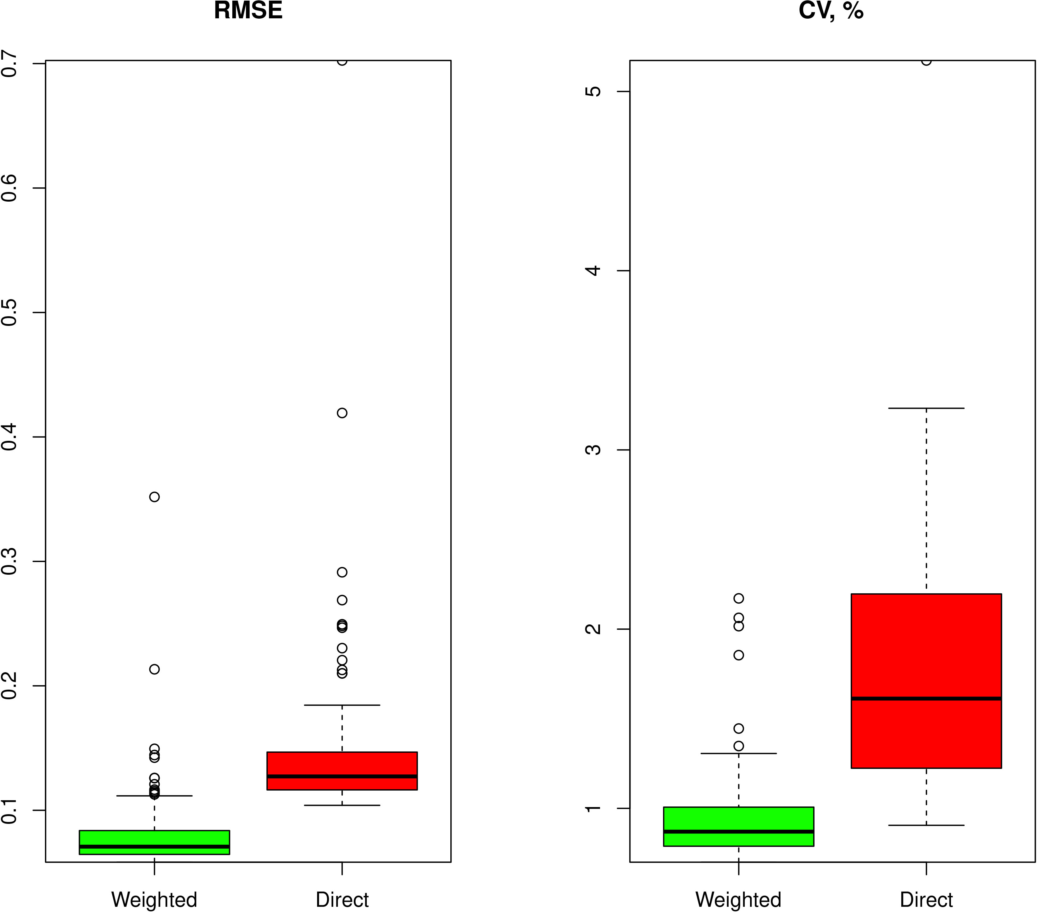
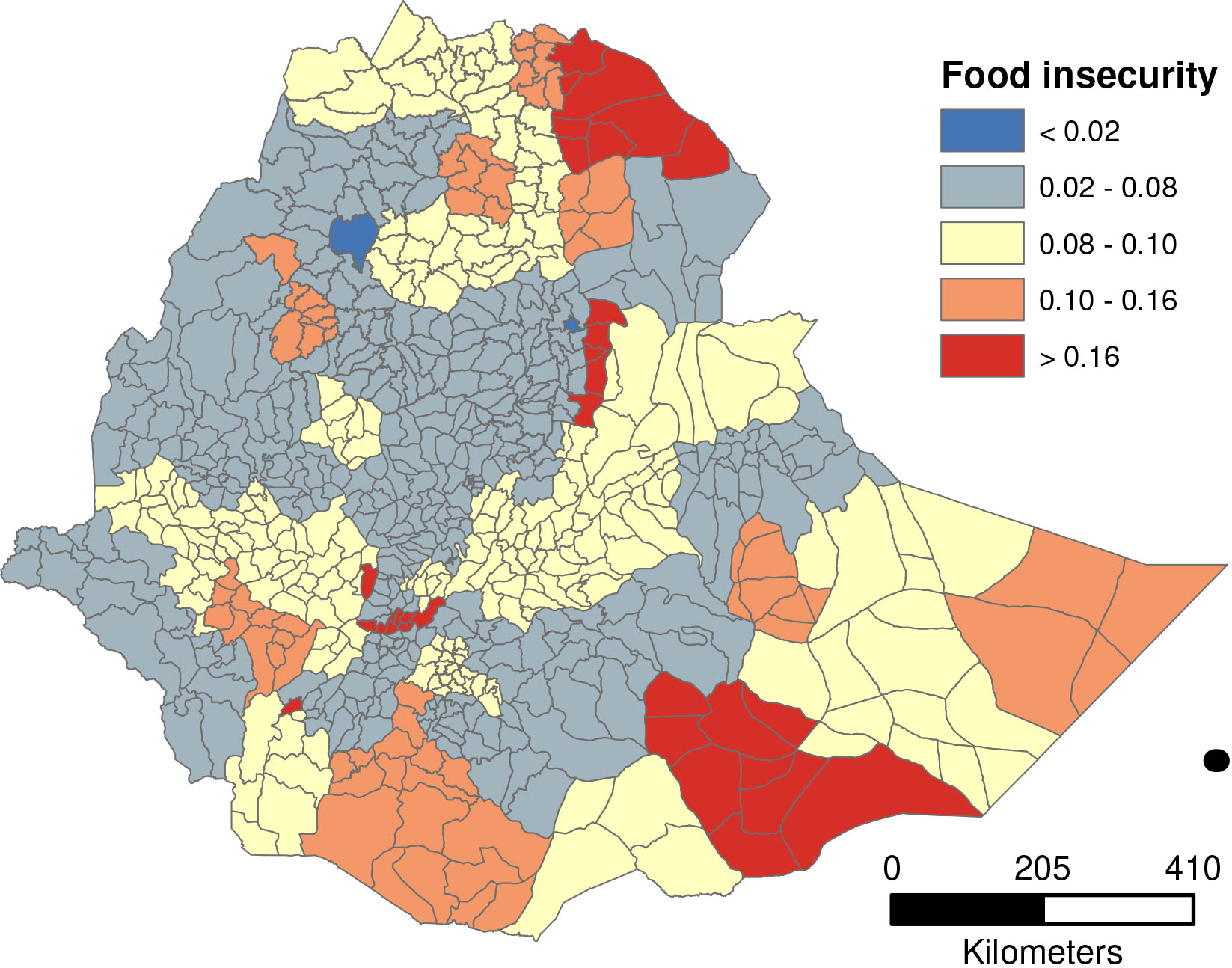
Figure 5.
A map of Ethiopia showing zonal level food insecurity estimates.
In the past two decades, food insecurity has received increased attention from various countries because of the severe financial crises [33]. Findings of the Fay-Herriot model analysis showed that women, households with greater than 12 years of schooling and household size less than five were significant determinants of food insecurity.
The relationship between women’s households and food insecurity was positive. In other words, for a unit increase on the women households keeping other covariates fixed, the food insecurity increases by 3.695. This result is not surprising in the Ethiopian context, as women have less access to education since they are responsible for domestic chores such as caring for children and the whole family [34]. Further, the majority of women are often forced to rely on casual labour due to their low educational status as better education provides higher chances of gaining better employment [35].
This study found a negative relationship between household heads who attended greater than 12 years of schooling and food insecurity. The study by [36] in Sidama district Southern Ethiopia found that wealth is highly correlated with education. They also found that education is strongly associated with the status of food security and hunger.
Self-employment was also found to be a significant predictor of household food insecurity in Ethiopia. There was a positive relationship with household food insecurity indicating that self-employment is largely a drive out of unemployment rather than being something driven by entrepreneurship [37]. More specifically, [37] reported declining trends in self-employment.
Finally, Fig. 5 shows the spatial mapping of zonal level household food insecurity obtained by the Fay-Herriot weighted approach. This map shows the degree of inequality concerning the distribution of household food insecurity in different zones. It is very crucial in identifying the zones and regions with low and high household food insecurity in Ethiopia.
4.Conclusion
Estimation of food insecurity related variables at the small area levels is a challenging statistical problem because sample sizes are too small and simple parametric models may be poorly captured the relationships between these variables [19]. There is a growing demand for accurate, reliable and cost-effective small area household food insecurity statistics among policy and decision-makers, private and public sector administrators using data from different sources. In this context, the Fay-Herriot weighted estimator has the potential to make a real impact. Therefore, this study has attempted to shed some light on the nature of household food insecurity in Ethiopian zones using the Fay-Herriot weighted estimator. This study used the data from the 2015/16 WMS and 2007 population and housing census of Ethiopia. It takes another step forward by reporting estimates of household food insecurity at the zone levels in Ethiopia, for the first time.
The results indicated that Ethiopian zones such as Amaro, Konso and Alaba contain the highest percentage of food-insecure households (above 30%) in 2015/16 and emerge as the most food-insecure zones in Ethiopia. These zones were identified as high priority zones for serious food insecurity and poverty alleviation interventions. In contrast, Addis Ketema, Nifas Silk, Bole, Arada, Yeka, Kirkos, Lideta, Kolfe, and Harari had the least food insecure households (below 5%) in 2015/16. These findings are not surprising since all of these zones except Harari are found in Addis Ababa, the economic hub of the country.
Moreover, the food insecurity map showed how household food insecurity varied by zones across Ethiopia. The map gave reliable information for the guidance of policy, resource allocation, and the planning and evaluation of the food insecurity measure programme. This information can be used by the government of Ethiopia for budget allocation and intervention of targeted zones. Furthermore, this information can also be the recommended tool for monitoring the progress of SDGs, launched in 2015, aim to end hunger, achieve food security and improved nutrition’ [2].
In summary, there was an overall clear gain of precision when using the weighted estimates based on the Fay-Herriot model instead of direct estimates. This indicated that weighted estimates of household food insecurity were more efficient and precise than the direct design-based estimates.
Finally, the findings demonstrate that accurate disaggregate household food insecurity statistics at small area level (zones) can be produced without more resources since this paper used the existing WMS and census datasets for this purpose [38]. Future research aimed at applying more advanced small area estimation techniques to improve the precision of household food insecurity estimates even at the fourth administrative levels (Woredas) in Ethiopia.
Acknowledgments
The author thanks the Central Statistical Agency of Ethiopia for the data used in the research. The findings of this working paper reflect the opinions of the author.
References
[1] | FAO, IFAD, UNICEF, WFP and WHO. The State of Food Security and Nutrition in the World 2018. Building climate resilience for food security and nutrition. Rome: FAO, (2018) . |
[2] | FAO, IFAD, UNICEF, WFP and WHO. The State of Food Security and Nutrition in the World 2019. Safeguarding against economic slowdowns and downturns. Rome: FAO, (2019) . |
[3] | Coleman-Jensen A, Nord M, Andrews M, Carlson S. Household Food Security in the United States in 2010. Economic Research Report No. 125. Washington, D.C. U.S. Department of Agriculture, Economic Research Service, (2011) . |
[4] | Burchi F, Scarlato M, d’Agostino G. Addressing food insecurity in Sub-Saharan Africa: The role of cash transfers. Poverty & Public Policy, (2018) ; 10: : 4. |
[5] | FAO, IFAD and WFP. The State of Food Insecurity in the World 2013. The Multiple Dimensions of Food Security. Rome: FAO, (2013) . |
[6] | FAO. Regional Overview of Food Insecurity Africa: African Food Security Prospects Brighter Than Ever. FAO: Accra, (2015) . |
[7] | World Food Programme. Comprehensive Food Security and Vulnerability Analysis (CFSVA). Executive Summary. Addis Ababa, Ethiopia, (2019) . |
[8] | Zerihun N, Getachew A. Levels of household food insecurity in rural areas of Gurage Zone, Southern Ethiopia: Journal of Agricultural Research, II, Bahir Dar, Ethiopia, (2013) . |
[9] | COMPACT 2025. Assessment of food security and nutrition situation. Roundtable Discussion, Addis Ababa, Ethiopia, (2016) . |
[10] | Ramakrishna G, Demeke A. An empirical analysis of food insecurity in Ethiopia. The case of North Wello. Africa Development Bank. (2002) ; XXVII: : 127-143. |
[11] | Balcha B. Food Insecurity in Ethiopia: The impact of socio-political forces. Aalborg University: Institut for Historie, Internationale Studier og Samfundsforhold, Aalborg Universitet, (2001) . |
[12] | CARE USA. Achieving Food and Nutrition Security in Ethiopia. Findings from the CARE Learning Tour to Ethiopia. Washington DC, January 19–24, (2014) . |
[13] | Rahmato D, Pankhurst A, van Uffelen J-G. Food Security, Safety Nets and Social Protection in Ethiopia. Forum for Social Studies, Ethiopia, Addis Ababa, (2013) . |
[14] | World Bank. World Bank Indicators. Retrieved from http://data.worldbank.org/indicator/SNon20October2019,2016. |
[15] | Lewis K. Understanding climate as a driver of food insecurity in Ethiopia. Climatic Change. (2017) ; 144: : 317-328. |
[16] | Gleixner S, Keenlyside N, et al. The el Niño effect on Ethiopian summer rainfall. Climate Dynamics. (2017) ; 49: : 1865-1883. |
[17] | Glantz HM. Usable science: Food security, early warnings and El Nino. Proceedings of the Workshop on ENSO/FEWS, (1994) . |
[18] | FAO. Situation report. Addis Ababa, Ethiopia, May 2016. Accessed on 30 October 2019 from http://www.fao.org/3/a-br072e.pdf. |
[19] | Pratesi M. Analysis of poverty data by small area estimation. John Wiley and Sons, (2015) . |
[20] | GeoDatos. Geographic coordinates of Ethiopia. Accessed on 05 November 2019 from https://www.geodatos.net/en/coordinates/ethiopia. |
[21] | CSA. Welfare and monitoring survey 2015/16. Statistical Report, I, Addis Ababa, Ethiopia, 2016. Accessed on 21 October 2019 from http://www.csa.gov.et/component/phocadownload/category/356-wms-2016. |
[22] | Esteban MD, Morales D, Perez A, Santamaria I. Small area estimation of poverty proportions under area-level time models. Computational Statistics and Data Analysis. (2012) ; 56: : 2840-2855. |
[23] | Yoshimori M, Lahiri P. A second-order efficient empirical Bayes confidence interval. The Annals of Statistics. (2014) ; 42: : 1233-1261. |
[24] | Fay RE, Herriot RA. Estimates of income for small places: An application of James-Stein procedure to census data. Journal of the American Statistical Association. (1979) ; 74: : 269-277. |
[25] | Henderson CR. Estimation of genetic parameters. Annals of Mathematical Statistics. (1950) ; 21: : 309-310. |
[26] | Rao JNK, Molina I. Small area estimation. Wiley Series in Survey Methodology, John Wiley and Sons, (2015) Inc., New York. |
[27] | Prasad NGN, Rao JNK. The estimation of the mean squared error of small area estimators. Journal of the American Statistical Association. (1990) ; 85: : 163-171. |
[28] | Datta GS, Lahiri P. A unified measure of uncertainty of estimated best linear unbiased predictors in small area estimation problems. Statistica Sinica, (2000) ; 10: : 613-627. |
[29] | Rivest LP, Belmonte E. A Conditional Mean Squared Error of Small Area Estimators. Survey Methodology. (2000) ; 26: : 79-90. |
[30] | Datta GS, Kubokawa T, Molina I, Rao JNK. Estimation of mean squared error of model-based small area estimators. Test. (2011) ; 20: : 367-388. |
[31] | Molina I, Marhuenda Y. sae: An R package for small area estimation. The R Journal. (2015) ; 7/1. |
[32] | Shiferaw YA, Galpin J. A Corrected Confidence Interval for a Small Area Parameter Through the Weighted Estimator under the Basic Area Level Model. JIRSS. (2019) ; 18: : 17-51. |
[33] | Endale W, Mengesha ZB, Atinafu A, Adane AA. Food Insecurity in Farta District, Northwest Ethiopia: A community based cross-sectional study. BMC Research Notes. (2014) ; 7: : 130. |
[34] | Burgess LG. When the personal becomes political: Using legal reform to combat violence against women in Ethiopia. Gender, Place & Culture. (2012) ; 19: : 153-174. |
[35] | Yitbarek K, Woldie M, Abraham G. Time for action: Intimate partner violence troubles one third of Ethiopian women. PLoS ONE. (2019) ; 14: : E0216962. |
[36] | Regassa N, Stoecker BJ. Household food insecurity and hunger among households in Sidama district, southern Ethiopia. Public Health Nutrition. (2011) ; 15: : 1276-1283. |
[37] | Haile GA. The nature of self-employment in urban Ethiopia. Policy Studies Institute, 50 Hanson Street, London, W1W 6UP, (2009) . |
[38] | Pereira LN, Mendes JM, Coelho PS. Model-based estimation of unemployment rates in small areas of Portugal. Communications in Statistics – Theory and Methods. (2013) ; 42: : 1325-1342. |


