
Administrative data informed donor imputation in the Australian Census of Population and Housing
Abstract
Response rates for official statistical collections are falling globally, placing increased emphasis on methods for handling missing data. At the same time, linked administrative data provides new opportunities for National Statistical Organisations. In 2016, the Australian Census of Population and Housing addressed unit non-response through nearest neighbour donor imputation. This method used dwelling and location characteristics to inform donor selection for each non-responding unit. This paper proposes a variation to the 2016 Census imputation method that incorporates administrative data to improve the selection of donors. Our method, Administrative Data informed Donor Imputation (ADDI), strengthens support for the assumptions of donor imputation, while limiting exposure to risks inherent in direct use of administrative data. We apply the ADDI method to the 2016 Census non-responding population, and demonstrate how the accuracy of imputation can be improved to produce higher quality statistics.
1.Introduction
Response rates for statistical collections have been falling globally [1]. The corresponding growth in the non-responding population creates challenges for official statisticians as the non-responding population typically differs from the responding population on important characteristics [2]. Addressing non-response is therefore necessary to avoid biased estimates [3].
There are two main types of non-response, item and unit non-response. Item non-response refers to a responding unit (usually a person, dwelling, or business) that is missing at least one collection variable. Unit non-response refers to a selected unit that is missing all collection variables. This paper focuses on donor imputation and its application within the Australian Bu- reau of Statistics (ABS) to address unit non-response in the Australian Census of Population and Housing.
Donor imputation replaces the missing value(s) in one unit (the recipient) with the response(s) from another ‘similar’ unit (the donor) [4]. This method fundamentally relies on identification of similar donor and recipient units. Donor imputation is most appropriate when the information that matches similar donors and recipients is associated with both the variable being imputed and the propensity of a unit to respond [5].
For non-responding units, the information available to identify similar donors is often limited. Administrative data, if joined to the non-responding units, can provide a range of new and valuable information to inform the identification of similar donor units. This paper proposes a method of incorporating this information into the donor imputation process.
1.1Imputation in the Australian Census of Population and Housing
The Australian Census of Population and Housing (the Census) collects information on the number of people and dwellings in Australia on Census night, and their basic demographics and characteristics. The Census is followed by the subsequent Post Enumeration Survey (PES), which is conducted after the Census enumeration period to provide an independent assessment of the coverage of the Census [6].
The Census is conducted based on place of enumeration, rather than place of usual residence. For private dwellings, Census responses are typically submitted at a dwelling level, containing data on all people present at the dwelling on Census night. A non-responding unit in the Census is a dwelling from which no valid response was received and that was identified by enumeration efforts as in scope and occupied on Census night.
Unit non-response in the 2016 Census was treated by imputation [7]. The method used is outlined below:
1. Information on all dwellings, such as dwelling structure (for example, a house or apartment), dwelling location (for example, a residential neighbourhood or retirement village) and geographic area, is compiled from the Census frame (which is based on the ABS Address Register [8]). This information is confirmed during enumeration, or collected where it was not available on the Census frame.
2. Imputation classes are constructed, stratifying dwellings by dwelling structure and dwelling location. Within an imputation class, non- responding dwellings (recipients) are matched to responding dwellings (donors) by the proximity of their geographic area. Random selection is used to pick a single donor dwelling from multiple eligible dwellings with the same proximity.
3. The number of people, and their age, sex, marital status and place of usual residence, from the donor dwelling is duplicated into the recipient dwelling. No other data items are imputed.
This method is a combination of random hot deck and nearest neighbour imputation [9]. Within each imputation class, geographic area is used to identify nearest neighbour donors. When there is only one nearest neighbour unit identified, it is selected as the donor. When there are multiple, equidistant nearest neighbour units identified, the donor is randomly selected from this pool.
In 2016, the Census dwelling response rate was lower than that in the 2011 and 2006 Censuses, resulting in higher rates of unit imputation. The 2016 PES indicated that the age distribution of the imputed population was skewed compared to that of the non-responding population [10]. This result indicates that the selection of donors based on dwelling information (dwelling structure, dwelling location and geographic area) could be improved. The implicit assumptions made by the imputation method regarding the mechanism for response missingness would be better supported by enhanced selection information.
1.2Missingness and imputation theory
Addressing non-response requires assumptions about the underlying mechanisms for response missingness. The simplest methods, such as complete case analysis, make the assumption of Missing Completely At Random (MCAR). This requires that the missingness is independent of all variables in the data set [3]. For social surveys, non-response analysis studies indicate that this is rarely a valid assumption [2].
Donor imputation relies on the more plausible Missing At Random (MAR) assumption. This requires that the missingness depends only on the observed variables and is independent of the unobserved, missing variables [11]. In non-response cases with many observed variables, such as item non-response, this can be a reasonable assumption. That is, when a range of information about the unit has been collected and only a particular item is missing, it can be reasonable to assume that the missingness depends on the range of collected information, and not on the missing item. This is particularly the case when the missing item can be implicitly modelled by other collected items.
For unit non-response, the only observed variables are those on the Census frame and other information collected during enumeration (see Section 1.1). It is difficult to support the assumption that unit missingness depends only on limited information about the dwelling, and not on other information such as the characteristics of the people resident at the dwelling.
The non-responding units in the 2016 Census were imputed under the MAR assumption with the observed variables of dwelling structure, dwelling location and geographic area. The PES found that non-response bias remained in the age estimates, which indicates that the MAR assumption was not well supported.
To address non-response bias through imputation, it is necessary to select observed variables that are strong predictors of the imputed variables and the propensity for a unit to respond [5, 9]. Administrative data, if joined to the Census frame, provides more observed variables for non-responding units, which can lend strength to the MAR assumption and provide more predictive match variables for nearest neighbour imputation.
There are many different imputation methods available [4]. The method of
1.3Administrative data in Australia
Administrative data is becoming increasingly available to, and sought after by, National Statistical Organisations (NSOs). Administrative data has been investigated in multiple applications for its ability to enhance statistical collections and releases [13]. The increased prevalence of, and continued improvements in, data linkage is a key enabler for these new approaches. Using administrative data in a methodologically sound manner presents a new challenge to NSOs: to maintain all dimensions of data quality while using data collected for non-statistical purposes. Generally, there are some quality challenges inherent in the use of administrative data for official statistics, which are discussed in detail in a number of papers [14, 15].
Some common limitations of administrative data include:
• Coverage bias: administrative data typically contains information about people interacting with a particular organisation or service. This usually results in incomplete or biased coverage of dwellings, and people within dwellings, compared to the general population.
• Stale data: administrative data custodians typically do not always remove stale or outdated data from their records. When people stop interacting with the relevant organisations or services, their information can remain on the administrative data for prolonged periods. This can create challenges when, for example, a person starts to interact again, and outdated and current records appear to co-exist on the data.
• Enumeration basis: administrative data sources, and particularly government data sources, typically hold information with respect to usual residence (given people are less likely to register for government services in temporary or short-term accommodation). This can present challenges when comparing such data sources to data collected on a non-usual residence basis, such as the Census, which is conducted on a place of enumeration basis.
• Location data: addresses in administrative data are often obtained for communication purposes. This results in data appearing at locations such as mailing addresses and post office boxes, and clustering at locations such as taxation accountant offices. These locations are typically not the locations of interest for official statisticians.
These limitations can be treated in various ways (see Section 2.1), although may not be able to be removed completely. Maximising the value of administrative data in official statistics requires adoption of methods that account for these limitations.
2.Methods
We propose an improvement to the 2016 Census unit imputation approach by drawing upon the strengths of administrative data. Our method, Administrative Data informed Donor Imputation (ADDI), incorporates administrative data to inform the choice of donors in donor imputation. Similar to the 2016 Census imputation approach, the ADDI method follows a nearest neighbour approach in combination with random hot deck imputation.
There are five main steps to implement the ADDI method:
1. Preparation of administrative data: cleaning and manipulating the data into a useful format;
2. Data linkage: joining the Census and administrative data at a unit record level;
3. Selection of match variables: determining which variables will be used to identify ‘similarity’ between donor and recipient units;
4. Selection of donors: using the match variables to identify an appropriate donor pool and donor for each recipient unit;
5. Imputation of variables: duplicating selected Census data from the donor unit to the recipient unit.
The steps are explored in more detail in the following sub-sections.
2.1Preparation of administrative data
Firstly, administrative data sources and variables that will provide information about the population of interest must be identified. For our analysis, the population of interest are those dwellings and people that were in scope of the 2016 Census. We identified two specific administrative data sources that have considerable coverage of this population: taxation and welfare government data.
The taxation data contains demographic and address information about people receiving a taxable income and certain other people. It also may contain a measure of the number of people (such as spouse and dependent children) who are assumed to reside at the same address. The data we used covers approximately 75 percent of the total Australian population and approximately 82 percent of Australian residential addresses. The coverage is skewed toward the demographics of the labour force, with reduced coverage outside of ages 18 to 55 years.
The welfare data contains demographic and address information about people receiving welfare payments. It also contains details of the category of welfare payment. The welfare payments have different eligibility requirements (such as the age and number of dependent children) so provide proxy demographic information for some non-recipients. The data we used covers approximately 73 percent of the total Australian population and approximately 77 percent of Australian residential addresses. Welfare data represents people receiving benefits, which is broadly families, pensioners, tertiary students, and low-income earners or unemployed people.
Once identified, the administrative data required cleaning and manipulation to address some limitations (see Section 1.3), and enable it to be used for statistical purposes. Preparation of the taxation and welfare data included the following activities:
• Coding information to standard categories or values. For example, encoding address text to standardised address identifiers, and coding date of birth to age in years at the time of the 2016 Census.
• Quality assurance of the data to identify, understand and, if possible, remove data issues. For example, removing duplicate records, records with no information, and outdated records with no evidence of recent interactions with the government services.
• Scoping the data to the population of interest. For example, removing records that represent people that were not in Australia or were deceased on Census night.
• Structuring the data in a useful format and deriving relevant variables. For example, summarising the person level administrative data at address level, such as deriving the count of males and females by age group at each address.
Once these activities were conducted, the clean and structured address level data from each administrative data source were ready to be combined through data linkage.
2.2Data linkage
There are a number of ways to link or join data, which vary in complexity [16]. For our analysis, the administrative and Census data were joined at the address level through match-merges of the standardised address identifiers (see Section 2.1). This is an operationally simple process to implement and followed the standard ABS procedures to ensure confidentiality, including the separation principle [17]. Identifying information (such as name and raw address) was not available to us and was not used for our analysis.
Once the Census and administrative data were joined in this way, approximately 90 percent of the occupied private dwellings on the Census had some administrative data attached.
2.3Selection of match variables
The administrative data join provides a wealth of variables to inform the choice of similar donors, but introduces a challenge in handing the increase in dimensionality, and incomplete coverage. As outlined in Section 1.2, the selection of appropriate match variables is integral to the effectiveness of donor imputation.
There are approaches to selecting match variables that utilise modelling to manage dimensionality, such as creation of a composite metric. This metric can reflect a modelled value of the variable to impute, such as a modelled age, or reflect the propensity of a unit to respond [5]. Alternatively, match variables can be selected manually, given some knowledge and analysis of the available variables. This latter, manual approach was implemented in our analysis.
The administrative data sources we used contained basic demographic variables, including age and sex. Our analysis indicated that the administrative age and sex variables were strong predictors for the 2016 Census age and sex variables among the responding population. In addition, age and sex are typically highly correlated with response propensity [2]. As the administrative age and sex variables are associated with variables being imputed (age and sex) and the propensity of a unit to respond, they are expected to be suitable match variables (see Section 1.2). We selected four variables (age and sex from each administrative data source) as match variables. This approach to selection constrains the number of match variables to grow linearly with the number of administrative data sources, rather than with the number of variables on each source.
The incomplete coverage of the administrative data sources we used meant that administrative data was not available for every non-responding unit. The coverage of administrative data is typically not random, and reflects real-world differences about the people who interact with particular organisations or services (see Section 1.3). Our analysis of linked administrative and 2016 Census data showed that whether or not a unit was represented on administrative data was associated with basic demographics and characteristics of the people resident. That is, responding units grouped by coverage or missingness on each administrative data source are more homogenous (in terms of Census age and sex) than the responding population as a whole. To capture this, we derived two administrative coverage indicator variables and selected these as match variables.
In summary, the administrative match variables we selected were the coverage indicator variables and the administrative age and sex variables. The 2016 Census match variables (dwelling structure, dwelling location, and geographic area) were kept to enable geographically close matches, and to improve matching for non-responding dwellings without linked administrative data.
2.4Selection of donors
Once the match variables were determined, donor units were selected for each recipient unit through a combined nearest neighbour and hot deck approach. Firstly, dwelling structure and dwelling location were used to form imputation classes. Within each imputation class, nearest neighbour units were identified using geographic area, administrative age and sex variables, and the coverage indicators. When a single nearest neighbour unit was identified, this unit was selected as the donor. When multiple, equidistant nearest neighbour units were identified, the donor was randomly selected from this donor pool.
Our nearest neighbour selection prioritised the coverage indicator and the administrative sex variable, followed by the proximity in administrative ages within the dwelling, and then proximity of geographic area. For simple integration into existing systems, we implemented the nearest neighbour selection through an iterative matching process. We classified the administrative age variables into age-range frequency bins at the dwelling level, and identified donors with exact matches to the recipient’s age-range frequency bins, coverage indicators, and smallest geographic area. If no exact match donors were found, we iteratively expanded the geographic matching area. This resulted in approximately 84 percent of non-responding units receiving a donor. For units without a match, we broadened the age-range frequency bins, and repeated the iterative geographic area search. Over two incrementally broader age-ranges, this resulted in approximately 14 percent of additional donor matching. Finally, for the remaining unmatched non-responding units (approximately 2 percent), we searched for nearest neighbour donors based on geographic area within the imputation classes (similar to the 2016 Census imputation method).
This nearest neighbour selection method can also be implemented via an explicit distance function, with higher relative weights for the coverage indicator and sex variables than those for the age variables and geographic area. The two approaches are equivalent when age-range frequency bins are utilised [5].
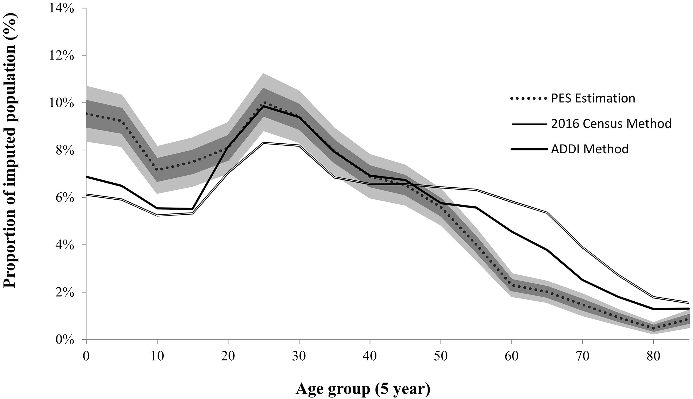
Figure 1.
Age distributions for the non-responding unit imputed population – 2016 PES population estimate, the 2016 Census imputation method and the ADDI method. Note: The PES Estimation shading illustrates one and two standard errors. Note: The 2016 Census imputation and ADDI methods are stochastic. Results for one implementation of each method are shown. Source: ABS data.
2.5Imputation of variables
Once a donor was selected, the donor unit’s Census responses were used to replace the recipient unit’s missing Census responses (for the items imputed on the Census: age, sex, marital status, and place of usual residence). The administrative data was only used to inform the selection of the donor and was not incorporated into the recipient’s imputed Census data. This is important as it reduces the exposure of the Census to the risks of the administrative data.
One such risk is the quality of the administrative data. Unlike some more aggressive uses of the administrative data, such as direct substitution, the ADDI method makes no assumption on the accuracy or completeness of the administrative data. The ADDI method, however, requires the more reasonable assumption that the characteristics of responding and non-responding units are similar, provided that they have similar administrative data.
Additionally, the unit non-response imputation occurs after the preliminary editing checks in the Census processing workflow. Therefore, no additional editing is required for the imputed records (which would be the case if the administrative data were imputed).
3.Results
The ADDI method was implemented to re-impute non-responding units in the 2016 Census. Our results were compared to the results of the 2016 Census imputation method and the 2016 PES. The PES results provide an estimate of the non-responding population that is independent to the Census. Imputation results that are closer to the PES results are indicative of less non-response bias, and better support of the MAR assumption.
As seen in Fig. 1, our results match the PES estimates more closely than the 2016 Census imputation method for all ages. The improvement is greatest between the ages of 18 to 55, corresponding to the highest coverage in the administrative data. The ADDI method draws strength from administrative data, so has less impact on populations not covered in the data sources utilised. Importantly, it does not do worse than the 2016 Census method for uncovered populations. This highlights the importance of identifying suitable administrative data sources (see Section 2.1).
4.Conclusions
Donor imputation is implemented in the Census to address unit non-response. However, limited information is available about non-responding units to inform the selection of donor units, and to support the assumptions of donor imputation.
The ADDI method, proposed by this paper, incorporates administrative data to inform the selection of donors in donor imputation. Introduction of administrative data expands the range of information available to form match variables, with which donors are selected via a nearest neighbour approach. The Census data for donors is imputed into recipient units, which limits the exposure of the Census to the risks inherent in direct use of administrative data.
When applied to the 2016 Census non-responding population, the results of the ADDI method are closer to the 2016 PES population estimate than the results for the 2016 Census imputation method. This indicates that the ADDI method further reduces non-response bias in the imputed population, through more predictive match variables and a more supported MAR assumption.
4.1Areas of future research
The research to date has demonstrated a number of benefits of the ADDI method. Focus areas of future research to enhance or further refine the method may include:
• Expansion of the range and coverage of administrative data sources used to form match variables. The ADDI method produced results closest to the 2016 PES results for the age range that had the most coverage on the administrative data sources. Incorporating additional administrative data sources with better coverage at other ages is expected to improve results for those ages.
• Use of composite metrics as match variables to inform the nearest neighbour selection of donors. Composite metrics can be produced from the administrative data variables to incorporate more information for the donor selection. The weighted contribution of each input variable can be determined through a regression of the administrative data on an informative Census variable for the responding population. This approach can simplify the selection of match variables and donors.
• Implementation of the ADDI method in combination with more direct methods such as administrative data substitution. This may be useful, for example, in situations where administrative data varies in quality, and therefore can be used for substitution for some but not all non-responding units.
Acknowledgments
We would like to thank Dr Siu-Ming Tam, Tania Mahoney, Nick Husek, Ben Ingram, Tamie Anakotta, and Ross Watmuff for their interest and support in helping us prepare this paper. We would also like to thank the ABS Census Futures team for their work on data access and preparation for the administrative data sources we used. Views expressed in this paper are those of the authors and do not necessarily represent those of the Australian Bureau of Statistics. Where quoted or used, they should be attributed clearly to the authors.
References
[1] | Tourangeau R, Plewes TJ. Nonresponse in social science surveys – a research agenda. Washington, DC: The National Academies Press; (2013) . 150. Available from: https://nap.edu/18293DOI:10.17226/18293. |
[2] | Groves RM, Couper MP. Nonresponse in household interview surveys. New York: Wiley; (2012) . |
[3] | Little RJ, Rubin DB. Statistical analysis with missing data. 2nd ed. New Jersey: Wiley; (2002) . |
[4] | Scholtus S. Theme – Donor Imputation, In: Handbook on Methodology of Modern Business Statistics. Eurostat, Collaboration in Research and Methodology for Official Statistics, (2017) Aug 2 [cited 2019 Jan 12]. p. 10. Available from: https://ec.europa.eu/eurostat/cros/content/imputation-donor-imputation-pdf-file_en. |
[5] | Andridge RR, Little RJ. A review of hot deck imputation for survey non-response, Int Stat Rev [Internet]. (2010) Apr [cited 2019 Jan 12]; 78: (1): 40-64. Available from: https://www.ncbi.nlm.nih.gov/pubmed/21743766 doi: 10.1111/j.1751-5823.2010.00103.x. |
[6] | Australian Bureau of Statistics (AU). 2940.0.55.002 – Information Paper: Measuring Overcount and Undercount in the 2016 Population Census, Jul 2016 [Internet]. Canberra (AU): Australian Bureau of Statistics; (2016) Jul 1 [updated 2016 Sep 28; cited 2019 Jan 12]. Available from: https://www.abs.gov.au/AUSSTATS/[email protected]/Lookup/2940.0.55.002Main+Features1Jul%202016. |
[7] | Australian Bureau of Statistics (AU). 2901.0 – Census of Population and Housing: Census Dictionary, 2016 – Derivations and imputations [Internet]. Canberra (AU): Australian Bureau of Statistics; (2016) Aug 23 [updated 2017 Oct 19; cited 2019 Jan 13]. Available from: https://www.abs.gov.au/ausstats/[email protected]/Lookup/2901.0Chapter29102016. |
[8] | Australian Bureau of Statistics (AU). 2008.0 – Census of Population and Housing: Nature and Content, Australia, 2016 – Address Register [Internet]. Canberra (AU): Australian Bureau of Statistics; (2015) Aug 20 [updated 2015 Dec 15; cited 2019 Jan 13]. Available from: https://www.abs.gov.au/ausstats/[email protected]/Lookup/by%20Subject/2008.0∼2016∼Main%20Features∼Collection%20operations∼93. |
[9] | Särndal CE, Lundström S. Estimation in surveys with nonresponse. West Sussex: Wiley; (2005) . |
[10] | Harding S, Jackson Pulver L, McDonald P, Morrison P, Trewin D, Voss A. Report on the quality of 2016 census data. Canberra (AU): Australian Bureau of Statistics, Census Independent Assurance Panel; (2017) Jun 27. 70. [updated 2015 Dec 15; cited 2019 Jan 13]. Available from: https://www.abs.gov.au/websitedbs/d3310114.nsf/home/Independent+Assurance+Panel/$File/CIAP+Report+on+the+quality+of+2016+Census+data.pdf. |
[11] | Rubin DB. Inference and missing data, Biometrika [Internet]. (1976) Dec [cited 2019 Jan 18]; 63: (3): 581-92. Available from: https://www.jstor.org/stable/2335739DOI:10.2307/2335739. |
[12] | Hastie T, Tibshirani R, Friedman J. The elements of statistical learning. 2nd ed. New York: Springer; (2017) . |
[13] | Wallgren A, Wallgren B. Register-based statistics – administrative data for statistical purposes. West Sussex: Wiley; (2007) . |
[14] | Tam SM, Clarke F. 1351.0.55.054 – Research Paper: Big Data, Statistical Inference and Official Statistics, Mar 2015 [Internet]. Canberra (AU): Australian Bureau of Statistics; (2015) Mar 18 [updated 2016 Jan 27; cited 2019 Jan 13]. Available from: https://www.abs.gov.au/ausstats/[email protected]/mf/1351.0.55.054. |
[15] | Special Issue on Coverage Problems in Administrative Sources, J Off Stat [Internet]. (2015) Sep [cited 2019 Jan 13]; 31: (3): 349-535. Available from: https://content.sciendo.com/view/journals/jos/31/3/jos.31.issue-3.xml. |
[16] | Harron K, Goldstein H, Dibben C. Methodological developments in data linkage. West Sussex: Wiley; (2016) . |
[17] | National Statistical Service (AU). The separation principle [Internet]. Canberra (AU): National Statistical Service; [cited 2019 Jan 13]. Available from: https://statistical-data-integration.govspace.gov.au/topics/applying-the-separation-principle. |


