
Estimating state level indicators from ICT household surveys in Brazil
Abstract
There is increasing demand from governments and civil society for more data and indicators for smaller territories and/or with higher frequency to help formulate and evaluate policies. At the same time, there is increasing availability of new data sources created by technologies such as Big Data. Some indicators are regularly produced by official and public statistics organizations, while others are demanded but currently not available, leading to substantial data gaps for many topics of interest. In some cases, existing data may lack the quality needed for its use in decision-making. All this coincides with the trend of diminishing resources available to collect data via traditional surveys, limiting sample sizes and increasing difficulties in producing the desired information. Aiming to meet part of this demand, this article compares four small area estimation methods to produce state-level estimates for two selected indicators using two editions (2014 and 2015) of the Survey on the Use of Information and Communication Technologies in Brazilian Households: ICT Households. The empirical study results indicate that using both temporal aggregation by pooling together samples of two consecutive years, and a composite estimator which borrows strength across larger regions leads to improved estimation of the target state-level ICT indicators.
1.Introduction
We live in an era of unprecedented data availability and accessibility, driven not only by incessant technology development, but also by increased demand from governments and civil society for more and more data and indicators to help formulate, measure, monitor and evaluate policies and decisions. An example of such demand is the set of Sustainable Development Goals Indicators – a framework of measures designed to monitor and evaluate progress in 17 different areas of human living conditions – defined by the United Nations Statistics Division.
A wide range of data and indicators is regularly produced by official and public statistics organizations to meet managers and decision-makers demands. Nevertheless, other data and indicators are demanded but currently not available, leading to substantial data gaps for many topics or areas of interest.
One increasing demand is the provision of statistics for smaller territories and/or with higher frequency. On one hand, this demand coincides with diminishing resources available to collect data, thus limiting sample sizes and increasing difficulties in producing the desired information. On the other hand, some existing data may lack the quality needed for its safe use in decision-making.
Since 2005, the Regional Center for Studies on the Development of the Information Society (Cetic.br), a department of the Brazilian Network Information Center (NIC.br), has collected data about access, use and appropriation of information and communication technologies (ICT) in several segments of society. The Survey on the Use of ICT in Brazilian Households (hereafter called the ICT Households survey) [1] measures the access and use of ICT by household residents in Brazil. With annual samples of close to 33,000 permanent private households, this survey is designed to produce reliable estimates for five Brazilian regions (North, Northeast, Southeast, South and Center-West). These regions represent macro divisions of the country that are made up of states (27 in total). Each state is formed by municipalities (cities and towns), which are the smallest formal government administrative units in Brazil (there are 5,570 municipalities).
Users of the ICT Households survey have been pressing for publication of the survey’s main indicators by the 27 Brazilian states. However, the precision of direct design-based estimates is low for many states, and such direct estimates are considered inadequate for general dissemination.
The aim of the present study was to find a simple method that allows the dissemination of ICT Households indicators by Brazilian states every year. Because the ICT Households survey produces a wide range of indicators and considering the tight timeline available for publication of survey estimates after data collection is completed, no explicit model-based approaches were considered. This decision is justified because model-based estimators, while potentially useful, require careful model fitting and checking to ensure that the resulting estimates meet the quality standards specified for the survey.
To assess feasibility, we applied four simple small area estimation (SAE) methods to obtain state-level estimates for two selected indicators from the ICT Households survey: proportion of households with computers, and proportion of households with Internet access. Details about the definitions of these target indicators are provided in [2] and in Section 2.1. We used data from two survey editions, 2014 and 2015, to produce the estimates in this article. The direct estimates are presented in Tables 3 and 4. The four estimation methods considered were: average of consecutive years – see [3]; pooling samples of consecutive years – see [3]; a single-year composite estimator considering the regions as yielding synthetic estimates; and a composite estimator based on pooling samples from two consecutive years, and using the regions as yielding synthetic estimates – see page 57 on [4]. The estimates derived from the various methods were evaluated using estimated mean squared error (MSE), and by comparing them with similar estimates produced by the 2015 edition of the National Household Sample Survey (PNAD) of the Brazilian Institute for Geography and Statistics (IBGE).
The PNAD was conducted to investigate socioeconomic characteristics of the Brazilian household resident population [5] and its main focus is the estimation of traditional labor force indicators. However, some questions on living conditions are also investigated, including a list of durable goods and services available in the household – including computer and Internet access – thus enabling estimation of a few ICT indicators. PNAD’s yearly sample of more than 150,000 permanent private households enables dissemination of reliable estimates for the 27 Brazilian states. The PNAD survey was discontinued by IBGE after the 2015 edition, and it was replaced by Continuous PNAD [6]. It is important to highlight that the ICT Households survey has many more ICT indicators than PNAD.
This article is divided into five sections. Section 2 describes the data sources. Section 3 presents the methods applied. Section 4 presents the results of the estimates and their analysis. In Section 5, we present the conclusions.
2.Data
The ICT Households survey utilizes a stratified multistage sample carried out independently every year. That is, a completely new sample is selected annually, which leads to the selection of different households. The target population is permanent private Brazilian households and their residents who are 10 years old or older. Detailed sampling design and weighting procedures for the ICT Households survey can be found in [1].
The frame used to design and select the ICT Households survey sample, which is the same as that used by PNAD, contains about 316,000 enumeration areas covering the whole country and is a product of the 2010 Brazilian Census. An enumeration area is defined by IBGE as a very small territory established for control purposes, such that the size of the territory and the number of households in each enumeration area should enable census data collection to be carried out by one interviewer within one month. Every enumeration area is contiguous, located entirely within the urban or rural portion of the territory of a single municipality. Each municipality is formed by a combination of enumeration areas. Also, each municipality is embedded in a state, and the union of states forms the regions that in turn make up the whole country.
Table 1
Sample size of enumeration areas and households for 2014 and 2015 ICT Households survey by region and by state
| 2014 | 2015 | |||
|---|---|---|---|---|
| Region | Enumeration areas | Households | Enumeration areas | Households |
| North | 221 | 2873 | 200 | 3000 |
| Northeast | 602 | 7826 | 615 | 9225 |
| Southeast | 719 | 9347 | 877 | 13155 |
| South | 331 | 4303 | 346 | 5190 |
| Center-West | 197 | 2561 | 176 | 2640 |
| State | ||||
| Rondônia | 31 | 403 | 18 | 270 |
| Acre | 15 | 195 | 15 | 225 |
| Amazonas | 37 | 481 | 38 | 570 |
| Roraima | 9 | 117 | 15 | 225 |
| Pará | 86 | 1118 | 84 | 1260 |
| Amapá | 14 | 182 | 15 | 225 |
| Tocantins | 29 | 377 | 15 | 225 |
| Maranhão | 61 | 793 | 71 | 1065 |
| Piauí | 38 | 494 | 36 | 540 |
| Ceará | 98 | 1274 | 97 | 1455 |
| Rio Grande do Norte | 35 | 455 | 39 | 585 |
| Paraíba | 47 | 611 | 45 | 675 |
| Pernambuco | 104 | 1352 | 98 | 1470 |
| Alagoas | 42 | 546 | 35 | 525 |
| Sergipe | 44 | 572 | 28 | 420 |
| Bahia | 133 | 1729 | 166 | 2490 |
| Minas Gerais | 170 | 2210 | 209 | 3135 |
| Espírito Santo | 61 | 793 | 47 | 705 |
| Rio de Janeiro | 168 | 2184 | 189 | 2835 |
| São Paulo | 320 | 4160 | 432 | 6480 |
| Paraná | 133 | 1729 | 130 | 1950 |
| Santa Catarina | 68 | 884 | 82 | 1230 |
| Rio Grande do Sul | 130 | 1690 | 134 | 2010 |
| Mato Grosso do Sul | 40 | 520 | 32 | 480 |
| Mato Grosso | 39 | 507 | 41 | 615 |
| Goiás | 67 | 871 | 70 | 1050 |
| Distrito Federal | 51 | 663 | 33 | 495 |
The stratification of the ICT Households survey is planned to ensure precise results for estimates by region (5 domains). The municipalities are grouped into 36 strata that are formed by each state, and in nine states (Pará, Ceará, Pernambuco, Bahia, Minas Gerais, Rio de Janeiro, São Paulo, Paraná and Rio Grande do Sul), the state-level groups are subdivided into ‘capital city and its metropolitan area’ and ‘non-capital cities’. The ICT Households survey considered the budget available, the desired quality of the measurements, and the size of the strata to empirically allocate the sample within strata. Due to cost considerations, sample allocation was larger for more populated areas and more accessible locations (e.g. state capital cities). Nevertheless, the survey estimates are expected to be unbiased given the use of probability sampling for all sampling stages and survey weights that reflect the disproportional sample allocation. In this study our aim was to obtain estimates for the 27 states and not for the 36 survey strata. The allocated sample size for each state is available in Table 1.
If a municipality is included in the sample with certainty – because it is a capital city or because of its large size (number of residents 10 years old or older) – then it becomes a stratum, and its enumeration areas are the primary sampling units (PSUs). If the stratum is formed by a collection of non-certainty municipalities, then the municipalities are the PSUs, and they are sampled using a probability proportional size (PPS) systematic sampling method – see [7] – where the size measure is the number of residents 10 years old or older. In both the certainty and sampled municipalities, the enumeration areas are also sampled by systematic PPS sampling where the size measure is the number of households.
Then, within each sampled enumeration area, the first operation carried out in the field is the compilation of an updated list of households to enable selecting the sample of households for interviewing. Households are sampled by simple random sampling without replacement (SRS). Selected households are then visited by the interviewers, who attempt contact and to obtain agreement to take part in the survey. For eligible households, the first step of the survey interview is the compilation of a list of the household residents. From such a household residents list, a single eligible resident is selected by SRS for interviewing. Therefore, all sampling stages are carried out using strict probability sampling procedures.
Field data collection is carried out by an outsourced contractor. The field work is closely monitored by NIC.br/Cetic.br, using a variety of methods, which include field visits to accompany selected data collection efforts, monitoring weekly and monthly control reports, and performing exploratory analysis of preliminary databases. In each of the years 2014 and 2015, 71% of the selected households answered the survey. Such similar rates result from the fact that the contractor providing the data collection services to the ICT Households survey has minimum household response rate targets to fulfill in each stratum. Although this is a contractual arrangement aimed at securing minimum levels of effort by the contractor, field work is carried out in strict adherence to the probability sampling protocols specified, and the response rate targets are used to monitor the efforts, not to change the sampling and contact protocols specified for the data collection.
The weighting procedure of the sample follows three steps:
1. Calculation of basic sampling weights using reciprocals of sample inclusion probabilities, accounting for all stages of sampling (municipalities, enumeration areas, households and residents);
2. Household non-response adjustment within enumeration areas assuming non-response was missing completely at random within each enumeration area – this means that no other variable was taken into account in order to adjust the weights, only the information of which census enumeration area the household belongs to; this was done because no other information is available for non-responding households;
3. Enumeration area non-response adjustment within strata assumed non-response was missing completely at random within each stratum; this was done for simplicity and considering the non-response of enumeration areas was very small; and
4. A final weight calibration by raking of the non-response adjusted weights was carried out to match known population totals obtained in the last published PNAD. The marginal distributions considered for calibration of household weights were: household location (urban or rural), ICT geography strata (36 strata), household size by number of residents (six categories: 1, 2, 3, 4, 5, 6 or more) and level of education of the head of the household (illiterate or Preschool, Elementary Education, Secondary Education or Tertiary Education).
Table 2
Sample size of enumeration areas and households for 2015 PNAD by region and by state
| 2015 | ||
|---|---|---|
| Region | Enumeration areas | Households |
| North | 1332 | 21442 |
| Northeast | 2659 | 43434 |
| Southeast | 2712 | 45546 |
| South | 1491 | 24532 |
| Center-West | 972 | 16235 |
| State | ||
| Rondônia | 170 | 2837 |
| Acre | 94 | 1642 |
| Amazonas | 240 | 3796 |
| Roraima | 57 | 1011 |
| Pará | 563 | 8697 |
| Amapá | 60 | 966 |
| Tocantins | 148 | 2493 |
| Maranhão | 205 | 3226 |
| Piauí | 127 | 2251 |
| Ceará | 457 | 7871 |
| Rio Grande do Norte | 129 | 2136 |
| Paraíba | 146 | 2444 |
| Pernambuco | 581 | 9110 |
| Alagoas | 128 | 2030 |
| Sergipe | 155 | 2508 |
| Bahia | 731 | 11858 |
| Minas Gerais | 813 | 13977 |
| Espírito Santo | 187 | 3087 |
| Rio de Janeiro | 689 | 11191 |
| São Paulo | 1023 | 17291 |
| Paraná | 457 | 7665 |
| Santa Catarina | 278 | 4511 |
| Rio Grande do Sul | 756 | 12356 |
| Mato Grosso do Sul | 158 | 2687 |
| Mato Grosso | 204 | 3268 |
| Goiás | 397 | 6617 |
| Distrito Federal | 213 | 3663 |
Source: Adapted from [14] – Prepared by the authors.
The PNAD sampling design and methods are detailed in [5]. The PNAD survey target population is formed by permanent private Brazilian households and their residents. The PNAD survey design is also a stratified multistage sample of permanent private households and their residents in Brazil. The sample size for the PNAD of close to 150,000 households (Table 2), as mentioned above, is much larger than that for the ICT Households survey. The coefficients of variation for the estimated Internet indicators are not available by state, only for regions (Table 7). For the estimates of households with computer indicator CVs are available for both states and regions (Table 7). Analysis of these CVs indicates that the ICT indicators estimates have good precision. Unfortunately, no other measures of quality (such as R-indicators, bias assessment etc.) are available for the PNAD.
The PNAD survey collects fewer ICT indicators and uses questions that are somewhat different from those in the ICT Households survey which will be discussed below. Nonetheless, PNAD’s estimates for the two selected indicators were compared to the estimates obtained by the four methods considered here.
3.Methods
First, we present some concepts, definitions and notation, required to describe the four alternative estimation methods considered. Then we present the expressions for the point estimates, and finally, the approaches used for the mean squared error (MSE) estimation.
3.1Concepts, definitions and notation
The main goal of this study is to choose a method to be used for providing estimates for domains that were not considered during the planning of the survey. For most states (the domains) the sample size is too small to provide reliable direct estimates. This is the reason to consider applying small area estimation methodology.
SAE methods often use a combination of data sources, models and/or estimation methods to increase the precision of desired estimates. The methods applied can be classified into model-based and design-based approaches. Model-based methods rely on models for the desired response using auxiliary information in order to increase precision. Frequently each response (indicator, in our case) is modeled separately. Therefore, if estimates are required for many indicators, the model specification, selection, fitting and checking may require substantial capacity and effort. Design-based methods use information from adjacent periods or areas (other small areas) and/or information about the design in order to increase sample size and precision.
Since users of the ICT Households survey have requested that NIC.br/Cetic.br starts publishing state-level estimates for well over 10 ICT indicators, we considered only design-based methods here, because they can provide a fast and easy way to deal with the large number of indicators at the same time.
The following notation was used throughout the paper:
•
•
•
•
•
•
•
•
•
•
•
•
Consider the finite population
For the ICT Households surveys in 2014 and 2015, parameter (i), proportion of households with computers, is obtained when the dummy variable takes the value 1 if the answer is “yes” to any of the following three questions:
• Is there a desktop computer in this household?
• Is there a portable computer or laptop in this household?
• Is there a tablet in this household?
The question used to calculate the indicator (ii) was:
• Is there Internet access in this household?
In the 2015 edition of PNAD, these indicators were captured by the following two questions:
• Are there microcomputers (including portables, such as laptops, notebooks, ultrabooks, netbooks and palmtops) in this household?
• Are any of these microcomputers used for Internet access?
Even with different questions used for capturing computer and Internet availability, estimates from PNAD were used for comparison with the estimates obtained using the four alternative methods considered here and applied to the ICT Households survey data. The four alternative methods considered by this study are as follows:
• Average of state-level estimates of two consecutive years;
• Estimates from pooled samples of two consecutive years;
• Single year composite estimates, combining region and state estimates; and
• Pooled sample composite estimates, combining region and state estimates.
For the composite estimation methods, the choice of weights is mostly developed in [4], page 57, and aims to reduce the MSE by balancing the unbiasedness of the direct estimator and the smaller variance of the synthetic estimators. The ICT Households survey was designed to provide good estimates for regions. Hence the direct estimates are unbiased for regions and should have small coefficients of variation (CV). The direct state-level estimates have much larger CVs, since the survey design did not consider the need for precise estimates at state-level.
Although the direct state-level estimates are unbiased under the design, small samples in some states (see Table 1) mean that there is the risk of having large differences between the estimates and the true values, because the small samples available do not represent well the corresponding populations. In order to test this possibility, we used the R-indicator – see [8] – which measures how the available sample differs from the planned sample.
The R-indicator can be defined by three different expressions, the most common being the standard deviation of the estimated response probabilities. In [8] it is based on the standard deviation of the selection probabilities. The R-indicator varies from 0 to 1. Table 6 shows the estimated state-level R-indicators with corresponding 95% confidence intervals.
Since the sample was not designed to produce estimates for states, it is possible that for some states with small samples the R-indicators are small, indicating samples which are imbalanced with respect to the corresponding populations.
That is why we chose the weights (
3.2Point estimation
Considering the survey weights
(1)
When the precision of the direct estimates does not meet the analytical needs or publication quality standards, combining samples that were not designed as rolling samples (see [9]), or borrowing information from adjacent or larger areas, can be considered if the combined results will meet the specified quality standards (see [3]). Therefore, we tried two methods that combine the samples of two consecutive years (temporal aggregation), one method that uses adjacent area information (spatial information), and one method that combines spatial and temporal information.
The simplest method uses the simple average of state-level estimates from two consecutive years to obtain improved state-level estimates given by:
(2)
Pooling samples [3] combines the microdata from the 2014 and 2015 ICT Households surveys into one data file, rescaling the original sampling weights by the factor 0.5, and calibrating the rescaled weights for the average population counts of the 2 years. The resulting pooled-samples estimator is given by:
(3)
where
The pooled estimator was inspired by the method used in the American Community Survey [10] to obtain multiyear estimates. It increases the sample size at the expense of having an estimate for a joint period that needs to be considered in the analysis, particularly if one aims for comparing estimates for different periods. While temporal aggregation introduces time-shift effects, we prefer to publish more reliable two-yearly estimates than single year estimates that are more volatile. In this choice we follow closely the American Community Survey [10] – see page 159.
The composite estimator, as defined in [4, p. 57], considers only data from the 2015 ICT Households survey (
(4)
where
(5)
and
The fourth method considers temporal and spatial aggregation, combining pooled sample estimates for states and regions in a composite estimator after pooling the samples from the 2014 and 2015 ICT Households surveys as described above. The direct estimates are obtained by applying Eq. (3) for the state-level and a similar expression to Eq. (5) for the region-level using the whole pooled sample – see Eq. (7). Then, these estimates are combined using varying weights as:
(6)
where
(7)
In Eq. (6) the weights
3.3MSE estimation
The MSEs of the proposed estimators were estimated in two different ways. First, we estimated the MSEs of the simple average (
(8)
The variances are estimated by:
(9)
Adding Eqs (3.3) and (9), the MSE estimate is:
(10)
Similarly, the MSE estimate for the pooled estimator is given by:
(11)
Variances for the single-year and pooled direct state-level estimators are estimated accounting for the complex sample design and the calibration using the survey package in R – see [11].
Table 3
Direct estimates and coefficient of variation from 2014 ICT Households survey by region and state
| Computer (%) 2014 | Internet (%) 2014 | |||
|---|---|---|---|---|
| Region | Estimate | CV | Estimate | CV |
| North | 33 | 7 | 35 | 8 |
| Northeast | 37 | 4 | 37 | 4 |
| Southeast | 59 | 2 | 60 | 2 |
| South | 57 | 3 | 51 | 4 |
| Center-West | 48 | 5 | 44 | 5 |
| State | ||||
| Rondônia | 34 | 7 | 33 | 20 |
| Acre | 31 | 12 | 25 | 12 |
| Amazonas | 35 | 13 | 35 | 13 |
| Roraima | 34 | 14 | 32 | 21 |
| Pará | 30 | 14 | 35 | 15 |
| Amapá | 52 | 12 | 50 | 20 |
| Tocantins | 35 | 20 | 38 | 16 |
| Maranhão | 19 | 16 | 15 | 19 |
| Piauí | 38 | 22 | 33 | 19 |
| Ceará | 38 | 6 | 33 | 9 |
| Rio Grande do Norte | 40 | 18 | 47 | 19 |
| Paraíba | 41 | 14 | 45 | 11 |
| Pernambuco | 43 | 7 | 45 | 6 |
| Alagoas | 35 | 7 | 47 | 12 |
| Sergipe | 29 | 14 | 27 | 12 |
| Bahia | 41 | 7 | 38 | 8 |
| Minas Gerais | 50 | 6 | 53 | 5 |
| Espírito Santo | 55 | 11 | 55 | 10 |
| Rio de Janeiro | 64 | 3 | 61 | 3 |
| São Paulo | 62 | 3 | 64 | 3 |
| Paraná | 53 | 5 | 46 | 8 |
| Santa Catarina | 68 | 4 | 59 | 7 |
| Rio Grande do Sul | 55 | 6 | 50 | 7 |
| Mato Grosso do Sul | 44 | 11 | 40 | 9 |
| Mato Grosso | 41 | 8 | 36 | 12 |
| Goiás | 41 | 12 | 38 | 11 |
| Distrito Federal | 76 | 4 | 74 | 4 |
Table 4
Direct estimates from 2015 PNAD and 2015 ICT Households survey by region and state
| Computer (%) | Internet (%) | ||||
|---|---|---|---|---|---|
| 2015 PNAD | 2015 ICT HH | 2015 PNAD | 2015 ICT HH | Comparable indicator | |
| North | 27 | 30 | 20 | 38 | 22 |
| Northeast | 30 | 38 | 26 | 40 | 30 |
| Southeast | 56 | 59 | 50 | 60 | 51 |
| South | 55 | 54 | 48 | 53 | 44 |
| Center-West | 49 | 44 | 42 | 48 | 36 |
| State | |||||
| Rondoônia | 35 | 14 | 28 | 18 | |
| Acre | 29 | 34 | 21 | 31 | |
| Amazonas | 31 | 33 | 22 | 42 | |
| Roraima | 37 | 44 | 28 | 63 | |
| Pará | 21 | 27 | 15 | 35 | |
| Amapá | 31 | 85 | 23 | 92 | |
| Tocantins | 29 | 23 | 22 | 34 | |
| Maranhaão | 18 | 21 | 14 | 30 | |
| Piauí | 24 | 37 | 18 | 31 | |
| Ceará | 28 | 45 | 23 | 38 | |
| Rio Grande do Norte | 39 | 50 | 34 | 50 | |
| Paraíba | 37 | 37 | 33 | 46 | |
| Pernambuco | 34 | 44 | 30 | 49 | |
| Alagoas | 27 | 46 | 23 | 48 | |
| Sergipe | 29 | 45 | 24 | 54 | |
| Bahia | 33 | 33 | 28 | 33 | |
| Minas Gerais | 48 | 52 | 41 | 53 | |
| Espírito Santo | 47 | 56 | 42 | 55 | |
| Rio de Janeiro | 53 | 62 | 49 | 62 | |
| São Paulo | 61 | 62 | 55 | 62 | |
| Paraná | 54 | 58 | 47 | 56 | |
| Santa Catarina | 58 | 54 | 53 | 56 | |
| Rio Grande do Sul | 53 | 49 | 46 | 48 | |
| Mato Grosso do Sul | 46 | 37 | 39 | 47 | |
| Mato Grosso | 39 | 42 | 32 | 42 | |
| Goiás | 44 | 39 | 38 | 48 | |
| Distrito Federal | 71 | 63 | 64 | 57 | |
Table 5
Proposed weights (
| CV (%) | ||||
|---|---|---|---|---|
| R-indicator | [0–5] | (5–10) | (10–20) | (20–100) |
| (0.00–0.60) | 0.4 | 0.3 | 0.2 | 0.1 |
| (0.60–0.70) | 0.6 | 0.5 | 0.5 | 0.4 |
| (0.70–0.85) | 0.8 | 0.7 | 0.6 | 0.6 |
| (0.85–1.00) | 0.9 | 0.8 | 0.7 | 0.6 |
Table 6
R-indicator with 95% confidence interval and CV for region and state-level direct 2015 ICT Households estimates
| Region | R-indicator with 95% CI | Computer CV (%) | Internet CV (%) |
|---|---|---|---|
| North | 0.839 (0.694–0.983) | 6 | 7 |
| Northeast | 0.895 (0.868–0.923) | 3 | 3 |
| Southeast | 0.919 (0.865–0.972) | 2 | 2 |
| South | 0.904 (0.824–0.984) | 5 | 5 |
| Center-West | 0.863 (0.775–0.952) | 2 | 2 |
| State | |||
| Rondoônia | 0.745 (0.436–1.000) | 31 | 26 |
| Acre | 0.668 (0.517–0.819) | 13 | 19 |
| Amazonas | 0.758 (0.583–0.932) | 10 | 7 |
| Roraima | 0.549 (0.379–0.720) | 12 | 7 |
| Pará | 0.823 (0.616–1.000) | 8 | 9 |
| Amapá | 0.534 (0.405–0.662) | 4 | 4 |
| Tocantins | 0.731 (0.566–0.895) | 16 | 10 |
| Maranhão | 0.779 (0.668–0.890) | 14 | 14 |
| Piauí | 0.940 (0.743–1.000) | 16 | 20 |
| Ceará | 0.874 (0.787–0.962) | 6 | 7 |
| Rio Grande do Norte | 0.843 (0.656–1.000) | 11 | 11 |
| Paraíba | 0.799 (0.651–0.946) | 9 | 9 |
| Pernambuco | 0.846 (0.728–0.964) | 5 | 5 |
| Alagoas | 0.818 (0.721–0.915) | 6 | 8 |
| Sergipe | 0.880 (0.715–1.000) | 7 | 7 |
| Bahia | 0.922 (0.813–1.000) | 5 | 5 |
| Minas Gerais | 0.908 (0.800–1.000) | 3 | 3 |
| Espírito Santo | 0.599 (0.428–0.770) | 10 | 10 |
| Rio de Janeiro | 0.930 (0.810–1.000) | 3 | 3 |
| São Paulo | 0.873 (0.815–0.931) | 3 | 3 |
| Paraná | 0.895 (0.764–1.000) | 4 | 4 |
| Santa Catarina | 0.821 (0.685–0.956) | 5 | 5 |
| Rio Grande do Sul | 0.895 (0.692–1.000) | 4 | 5 |
| Mato Grosso do Sul | 0.718 (0.588–0.848) | 14 | 11 |
| Mato Grosso | 0.758 (0.517–0.999) | 11 | 11 |
| Goiás | 0.801 (0.651–0.950) | 8 | 7 |
| Distrito Federal | 0.869 (0.614–1.000) | 7 | 11 |
Table 7
Coefficients of variation (%) of the PNAD 2015 estimates
| 2015 | ||
|---|---|---|
| Region | Computer CV (%) | Internet CV (%) |
| North | 2 | 3 |
| Northeast | 1 | 2 |
| Southeast | 1 | 1 |
| South | 1 | 1 |
| Center-West | 2 | 2 |
| State | ||
| Rondônia | 5 | |
| Acre | 7 | |
| Amazonas | 5 | |
| Roraima | 8 | |
| Pará | 4 | |
| Amapá | 9 | |
| Tocantins | 7 | |
| Maranhão | 7 | |
| Piauí | 8 | |
| Ceará | 3 | |
| Rio Grande do Norte | 5 | |
| Paraíba | 6 | |
| Pernambuco | 3 | |
| Alagoas | 6 | |
| Sergipe | 5 | |
| Bahia | 3 | |
| Minas Gerais | 2 | |
| Espírito Santo | 4 | |
| Rio de Janeiro | 2 | |
| São Paulo | 1 | |
| Paraná | 2 | |
| Santa Catarina | 2 | |
| Rio Grande do Sul | 2 | |
| Mato Grosso do Sul | 4 | |
| Mato Grosso | 5 | |
| Goiás | 3 | |
| Distrito Federal | 2 | |
Source: Adapted from [14] – Prepared by the authors.
Table 8
Median of root-MSE (%) for state-level estimates by indicator and by method
| Method | Computer (%) | Internet (%) |
|---|---|---|
| Direct | 2.99 | 3.57 |
| Average of two consecutive years | 4.34 | 6.04 |
| Pooled samples | 3.76 | 4.16 |
| Composite of single year | 4.04 | 4.58 |
| Composite of pooled sample | 3.07 | 4.12 |
The MSE estimates for the composite estimators were obtained using Eq. (4.3.2) on page 57 in [4] and using the bootstrap procedure proposed in [12], adapted to our survey situation. The first step of the bootstrap procedure yields the population of PSUs in each stratum by replication of PSUs selected in the sample. If the PSUs within the stratum are municipalities, this step ends up with as many municipalities as there are in the stratum population, excluding the certainty ones. For the certainty municipalities that play the role of strata, their PSUs consist of census enumeration areas. The second step of the bootstrap procedure consists of constructing the population of census enumeration areas, replicating the enumeration areas in the sample in each municipality selected in the first step. The second step ends up with as many enumeration areas as there are in municipalities in the sample.
Applying this procedure would lead to incorrect results. The selection of census enumeration areas for the ICT Households sample is with probabilities proportional to size but considers different size measures for urban and rural areas. In rural areas the measure of size is half the measure of size used for urban areas (in both cases, the number of households listed in the 2010 Census is the baseline size measure). That is, for two census enumeration areas with the same number of households, one urban and one rural, the urban area would have twice the probability of being selected as the rural one.
It turns out that this choice of selection probabilities in the ICT Households survey is not dealt with by the method described in [12]. To accomplish the same objectives are those described in [12], we needed to divide the bootstrap population of census enumeration areas into rural and urban groups within each stratum, so that rural and urban enumeration areas could appear in the bootstrap sample in the same numbers as they occur in the population.
Based on the methodology described in [12] adjusted to the case of the ICT Households survey, 500 samples without replacement and with equal probability were selected in each stratum from the database of replicated municipalities and census enumeration areas, with the same sample size as that used in the original sample. In each selection, we used the survey respondents in order to calculate the statistics of interest: composite estimates for both indicators, as described in Eqs (4) and (6), and their estimated MSE:
(12)
After this procedure, we calculated the average of the point estimates and the average of the MSE from each replicate to obtain the final MSE estimate for each state. We also obtained the 2.5% and 97.5% quantiles of the point estimates to obtain empirical 95% confidence limits.
4.Results
The data on the ICT indicators were collected in PNAD using different questions when compared to the ICT Households survey. However, direct estimates by Brazilian region (see Tables 3 and 4) or for the whole country are not too different between the two surveys. Larger differences appear when comparing direct state-level estimates (see Tables 3 and 4).
Figure 1.
Comparison of state-level point estimates for computer indicator with 2015 PNAD.
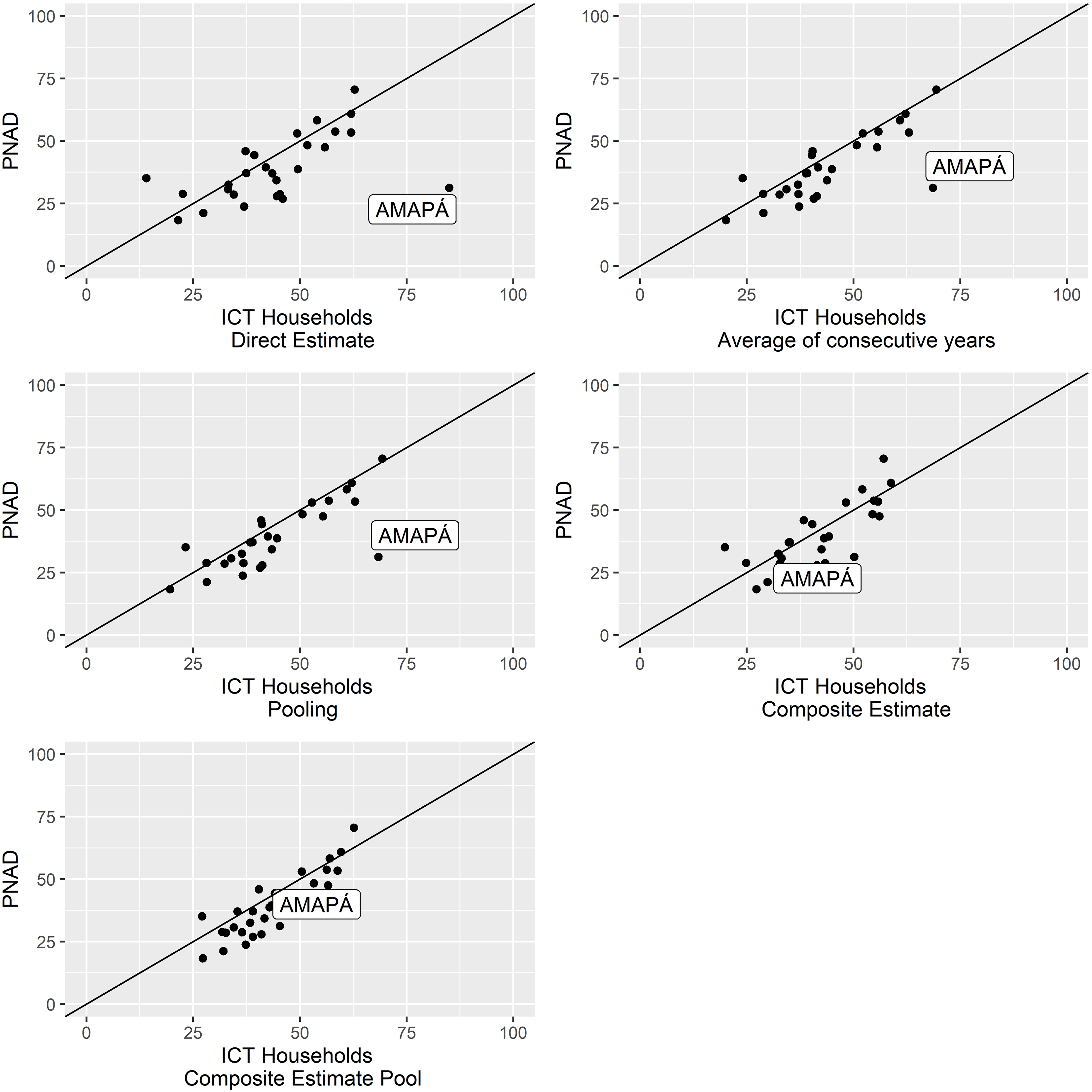
Figure 2.
Comparison of state-level point estimates for Internet indicator with 2015 PNAD.
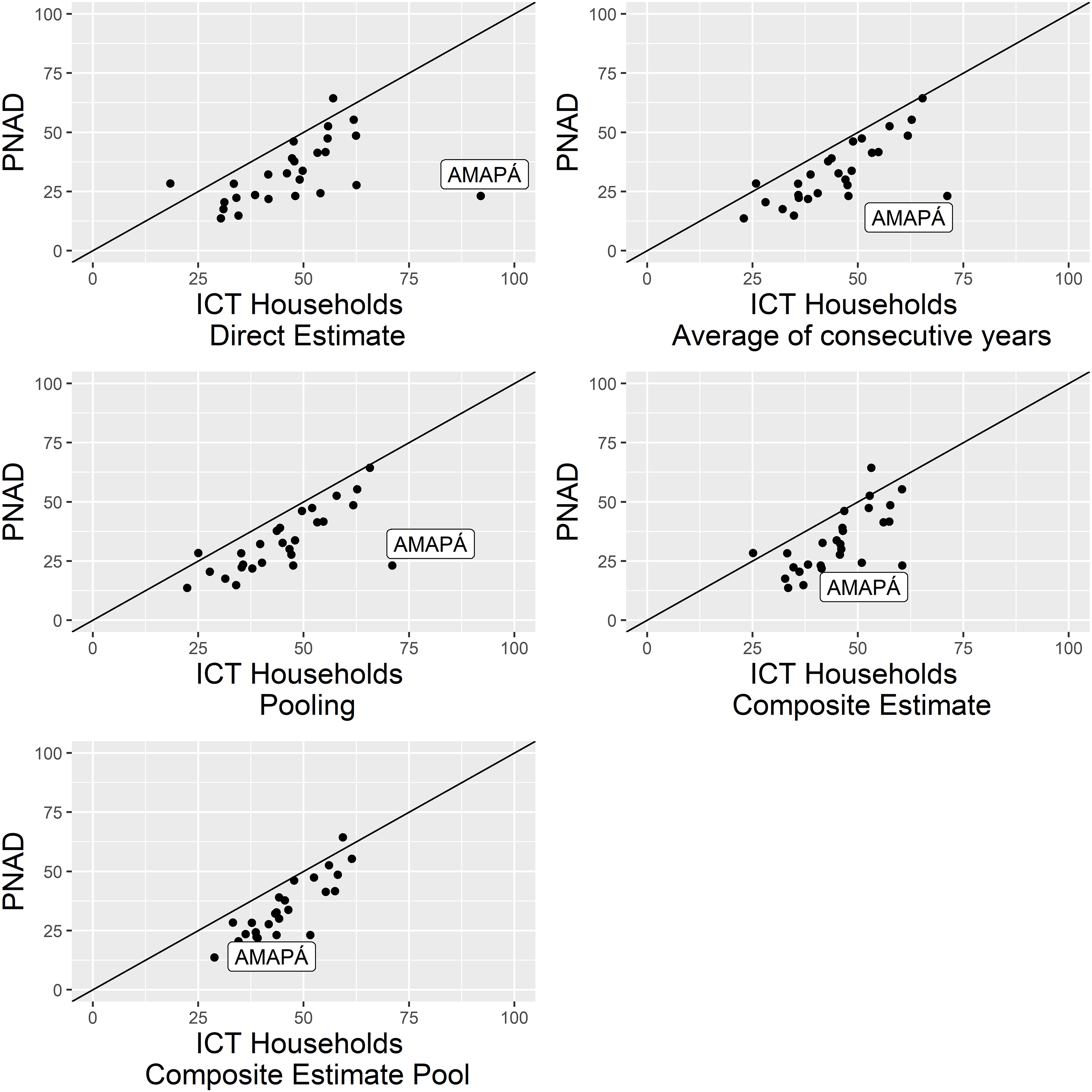
Figure 3.
State-level pooled sample composite estimates and 95% confidence limits for computer indicator.
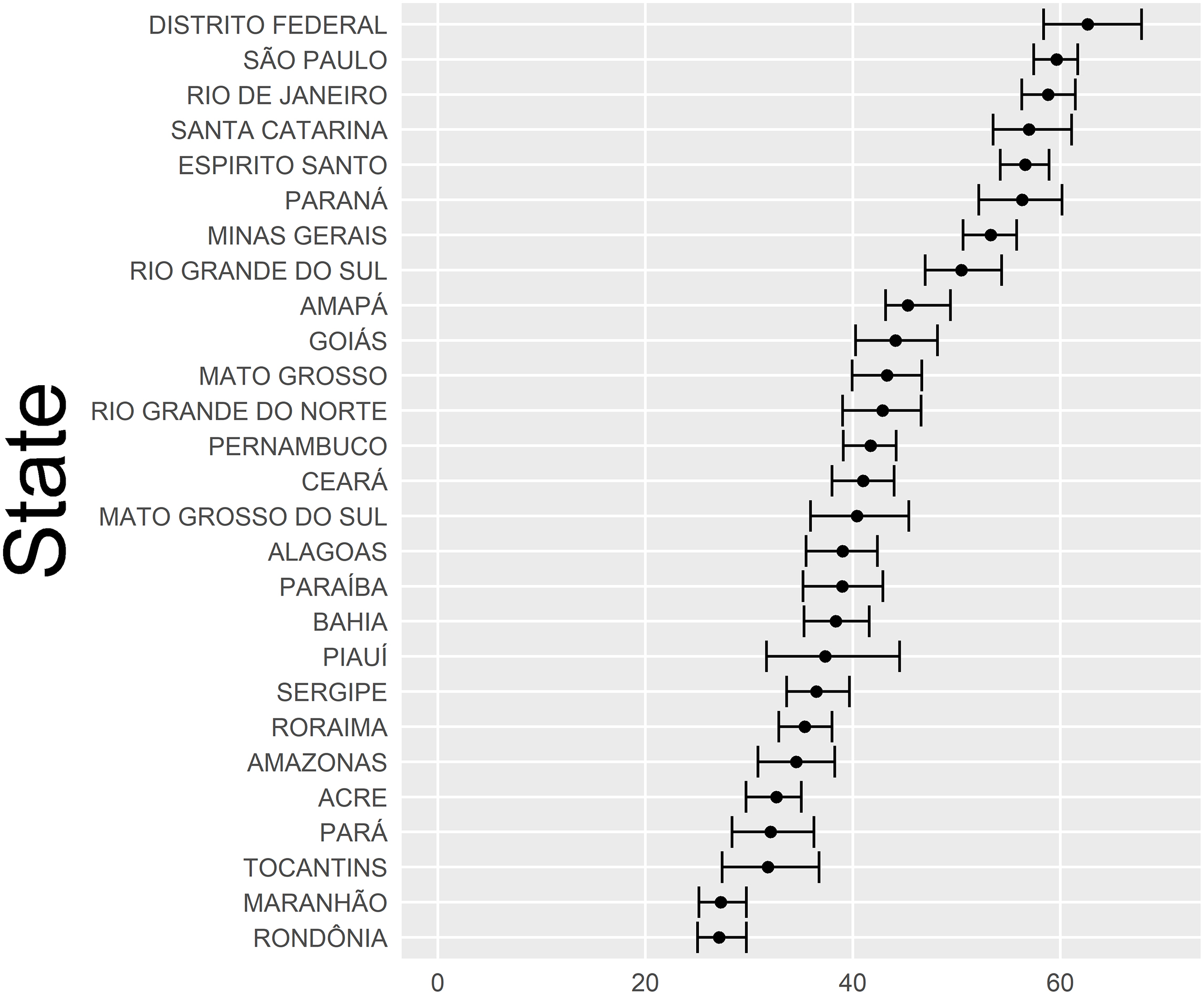
Figure 4.
State-level pooled sample composite estimates and 95% confidence limits for Internet indicator.
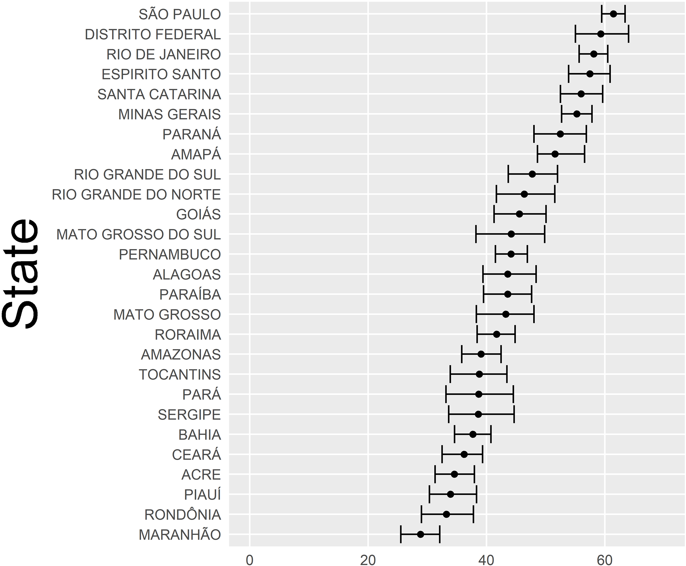
Figure 5.
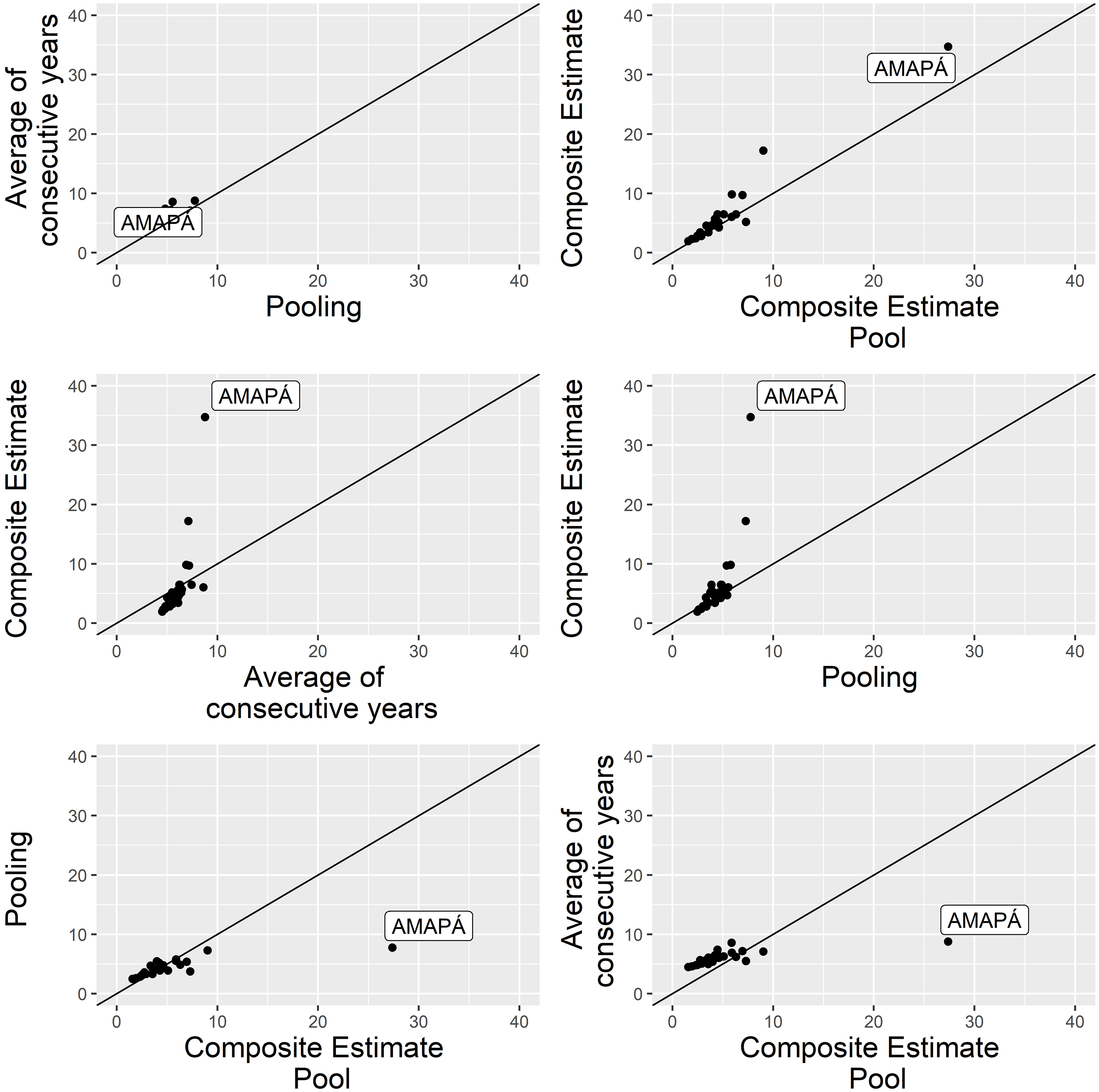
Comparison of root-MSE of SAE estimates for computer indicator.
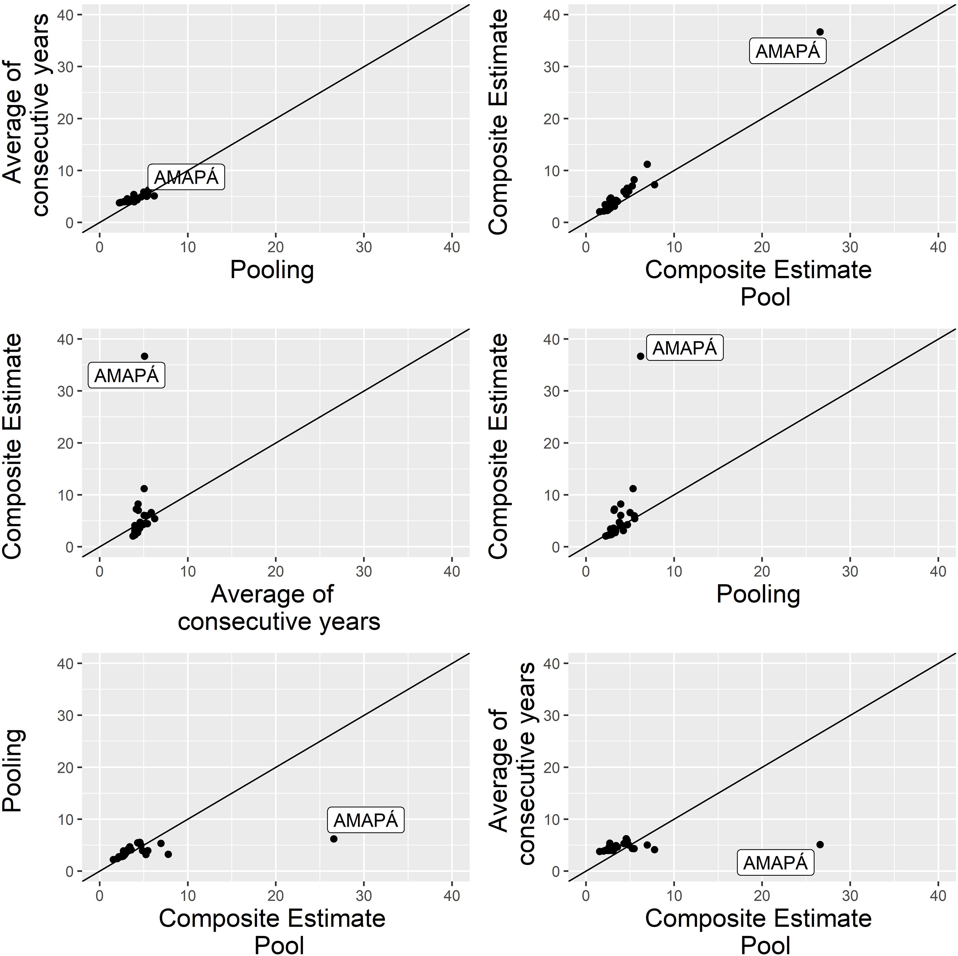
Figure 6.
Comparison of root-MSE of SAE estimates for Internet indicator.
Regarding the computer availability estimates, for most regions (except the Northeast) the differences fall within margins of error. The ICT Households survey gives larger estimates for households with Internet access, because it considers the possibility of having Internet access in a household even if it is not accessed by a microcomputer (as is the case for PNAD). In order to evaluate if the differences exceed the margins of error, we included in Table 4 a ‘comparable’ estimate – it is marked with * – for the ICT Households 2015 Internet indicator in which we consider that there is Internet access just for households in which there is at least one computer. Considering this ‘comparable indicator’, the differences do not exceed the margins of error for all regions. This ‘comparable indicator’ is not used in the rest of the work, because ICT Households Survey adheres to the international recommendation (see [2]).
In contrast, the direct estimates by states are quite different, mostly for Brazilian states in the North and Northeast regions where the ICT Households survey sample is small due to the high cost of collecting data. The sample sizes are in Tables 1 and 2 and the estimates are in Tables 3 and 4.
Table 6 shows the ICT Households survey CVs of the direct state-level estimates and the R-indicators [13]. For some states the ICT Households available samples yielded small R-indicators, indicating that the direct estimates for these states are derived from imbalanced samples, something which is not captured when considering simple standard error or CV estimates. On the other hand, for some states the CVs for the direct estimates are high, leading to wide margins of error and large uncertainty in the estimates. CVs range from 3% to 31%, and R-indicators from 0.53 to 0.94. The smallest R-indicator was observed for the state of Amapá in the North region of Brazil, suggesting that the sample available for this state is not sufficiently representative.
These contrasting quality indicators (CV
The direct estimates have smaller MSE estimates, but these did not include a bias component, which in many cases would be needed, given that the corresponding state R-indicators suggest that there are important differences between the available sample and the population. Hence, the composite of pooled samples method performed best among the approaches considered, when the direct estimator is left out.
In addition, we plotted the state-level estimates for the chosen method and the direct estimates against PNAD’s estimates to evaluate the patterns (see Figs 1 and 2). We clearly see the large difference for Amapá state. The composite of pooled samples estimate is in line with PNAD, whereas the direct estimate for this state is quite far off.
The pooled-sample composite state-level estimates plus their empirical 95% confidence intervals for the proportion of households with computers and for the proportion of households with Internet are shown in Figs 3 and 4 respectively. Margins of error are small (less than 5%) or modest (5 to 10%) for most states, and generally smaller for the proportion of households with computer. Survey analysts consider such estimates adequate for public dissemination.
Table 9
Correlation between state-level estimates from ICT HH and PNAD by indicator and by method
| Method | Computer | Internet |
|---|---|---|
| Direct | 0.572 | 0.446 |
| Average of two consecutive years | 0.782 | 0.713 |
| Pooled samples | 0.789 | 0.728 |
| Composite of single year | 0.766 | 0.672 |
| Composite of pooled sample | 0.887 | 0.864 |
5.Conclusion
According to the R-indicator, six state samples from the ICT Households survey appear to represent poorly the corresponding state populations (see Table 6). Apparently, our pooled-sample composite estimation reduced the representativeness problem, but at the cost of modestly increased root-MSE (Figs 5 and 6). However, our root-MSE estimates for the direct estimator include rather naïve estimates for its bias, and hence, we consider the pooled-sample composite estimator root-MSE estimates as more reliable.
Pooling samples and averaging data for consecutive years increases the sample sizes at the cost of adding a time-trend bias. Our choice is to disseminate the estimates as regarding a two-year period, in a similar way as is done by the American Community Survey, for example. Also, for some states this did not compensate the representativeness problem. On the other hand, composite estimation includes a bias originating from the synthetic ‘regional’ estimator.
The pooled-sample composite estimator borrows strength across both time and space. The gains in precision and in the comparison with the point estimates from PNAD with this estimator are sufficient to enable dissemination of state-level estimates. Analyzing Figs 1 and 2, we see that the estimates from pooled-sample composite method are closer to the PNAD estimates for all states in comparison to all other approaches, including for Amapá state, which was the state with lowest R-indicator (Table 6). This can be confirmed in Table 9, which shows the correlation between state-level PNAD and ICT Households survey estimates obtained by all estimation methods considered. The correlation between direct ICT Households and PNAD estimates is equal to 0.572 for computer and 0.447 for Internet. For the pooled-sample composite and PNAD estimates the correlations are 0.887 and 0.864 respectively.
Hence, the pooled-sample composite estimator will be adopted to calculate the state-level estimates for the various indicators from the ICT Households survey, that will be disseminated to the public. Since NIC.br/Cetic.br data users have requested regular publication of state-level estimates for ICT indicators, we suggested the adoption of a sample-design that enables faster accumulation of sampled PSUs to obtain more reliable state-level estimates using the proposed estimation approach. As an extension of this work, we will study the possibility of producing estimates for states, following this methodology, but benchmarking to the estimates for regions averaged over two consecutive years.
References
[1] | Brazilian Network Information Center (NIC.br). Survey on the use of information and communication technologies in Brazilian households: ICT Households 2015. Brazilian Internet Steering Committee, (2016) . [cited 2020 March 10]. Available from: http://cetic.br/arquivos/domicilios/2015/domicilios/. |
[2] | International Telecommunications Union. Manual for measuring ICT access and use by households and individuals 2014. ITU, (2014) . [cited 2020 March 10]. https://www.itu.int/dms_pub/itu-d/opb/ind/D-IND-ITCMEAS-2014-PDF-E.pdf. |
[3] | Thomas S, Wannell B. Combining cycles of the Canadian community health survey. Health Reports, 20: (1) ((2009) ): 53. |
[4] | Rao JNK. Small area estimation. John Wiley & Sons, (2003) . |
[5] | Brazilian Institute of Geography and Statistics (IBGE). National Household Sample Survey. IBGE, (2016) . [cited 2020 March 10]. Available from: http://downloads.ibge.gov.br/downloads_estatisticas.htm. |
[6] | Brazilian Institute of Geography and Statistics. Continuous National Household Sample Survey. IBGE, (2018) . [cited 2020 March 10]. Available from: https://www.ibge.gov.br/en/statistics/social/housing/18083-annual-dissemination-pnadc3.html?=&t=o-que-e. |
[7] | Särndal C, Swensson B, Wretman J. Model assisted survey sampling. New York: Springer Verlag, (1992) . |
[8] | Schouten B, Cobben F, Bethlehem J. Indicators for the representativeness of survey response. Survey Methodology, 35: (1) ((2009) ): 101-113. |
[9] | Kish L. Cumulating/combining population surveys. Survey Methodology (Statistics Canada, Catalogue 12-001), 25: (2) ((1999) ): 129-38. |
[10] | U.S. Census Bureau. American Community Survey Design and Methodology (January 2014). [cited (2020) March 10]. Available from: https://www2.census.gov/programs-surveys/acs/methodology/design_and_methodology/acs_design_methodology_report_2014.pdf. |
[11] | Lumley, Thomas. Complex Surveys: A Guide to Analysis Using R. Hoboken: John Wiley & Sons, (2010) . 276. |
[12] | Mecatti F. Bootstrapping unequal probability samples. Statistica Applicata, 12: (1) ((2000) ): 67-77. |
[13] | Santos MPR dos, Pitta MT, Silva DBN. Indicators of representativeness in survey on the use of information and communication technologies in Brazilian households. Statistical Journal of the IAOS, 1: ((2020) ): 1-10. doi: 10.3233/SJI190509. |
[14] | Brazilian Institute of Geography and Statistics (IBGE). Pesquisa nacional por amostra de domicílios: síntese de indicadores 2015. Coordenação de Trabalho e Rendimento, Diretoria de Pesquisas, (2016) . |


