When adjusting for the bias due to linkage errors: A sensitivity analysis

2.1The probabilistic record linkage

The fundamental theory of probabilistic record linkage is given by Fellegi and Sunter [5]. Given two lists, say L1 and L2, of size N1 and N2, let Ω={(a,b),a∈L1 and b∈L2} be the set of all possible pairs, whose size is |Ω|=N1×N2. The process of linking lists L1 and L2 can be seen as a classification problem where the pairs in Ω have to be assigned to two independent and mutually exclusive subsets M and U, such that:

M is the link set (a=b)

U is the non-link set (a≠b).

In order to assign pairs to the sets M or U, a number, say K, of common identifiers, called the linking variables, are selected and, for each pair of records, a comparison vector γ={γ1,γ2,…,γK} is obtained. The ratio r between the conditional probability of γ given that the pair belongs to the set M and the conditional probability of γ given that the pair belongs to the set U

is used for classifying the pairs. The two probabilities m and u can be estimated, for instance as proposed by Jaro [6], assuming the true link status is a latent variable and using the EM algorithm. The pairs for which r is greater than an upper threshold Tm are assigned to the set of linked pairs, M*; the pairs for which r is smaller than a lower threshold Tu are assigned to the set of unlinked pairs U*; when the ratio r falls within the range (Tu,Tm), no decision is made and the pair is resolved by a clerical revision.

The thresholds Tu,Tm are chosen to minimize the false link probability, η, and the false non-link probability, 1-α, defined as follows:

The described linkage model also allows for the evaluation of the probability that a link is correct given that the link is assigned, the so-called true match rate:

The parameter λ in Eq. (3) plays a fundamental role in the adjustment for linkage errors, as shown in the following section. However, the role of the probability of missing a link α is very relevant, as the results show in Section 4.3.

4.1Adjusted estimators for linkage errors in regression models

Let y be the target variable and X be the matrix of auxiliary variables observed on the same units, assuming a linear relationship between the target variable and the covariates y=X⁢β+ε, where β is the vector of regression coefficients and ε is the vector of i.i.d. random variables with E⁢(ε)= 0 and 𝑉𝑎𝑟⁢(ε)=σ2.

Due to linkage, the observed target variable is y∗ instead of true unobserved y. Then, the standard estimator of the regression coefficient applied to the linked data is:

Chambers [11] defines an exchangeable linkage errors model by assuming that the probability of correct linkage is the same for all records, or at least the probability is the same in groups partitioning the whole observations.

Chambers [11] models the relationship between the probabilistically linked data and the true data: y∗=A⁢y, where A is an unknown random permutation matrix, under the following assumptions:

As mentioned in Section 3.1, Scheuren and Winkler [8] propose a biased corrected OLS estimator of β, formulated by Chambers [11] as:

where the matrix E is the expected value of the matrix A.

Alternatively, modeling the relationship between the linked data and the covariates, under the assumption of homoscedasticity, Lahiri and Larsen [10] propose the following estimator:

To take also into account the heterogeneity, Chambers [11] proposes a Best Linear Unbiased Estimator (BLUE) of β:

where Σ=σ2⁢I+V is the variance matrix of y∗, and V is the variance 𝑉𝑎𝑟⁢(A⁢X⁢β).

For the linear logistic model, logit⁢(p)=X⁢θ, where p is the expected value of a binary variable y, a GEE approach is applied in Chambers [11]; the bias corrected form of the estimating functions is

where f⁢(θ)=EX⁢(y) and G⁢(θ) is a function of θ and X.

Under perfect linkage, the logistic model is fitted via ML with G⁢(θ)=XT then Eq. (8) can be specified as:

Alternatively, the function G⁢(θ)=XT⁢ET corresponding in the linear case to the Lahiri and Larsen estimator in Eq. (6), leads to:

and G⁢(θ)=XT⁢D⁢(θ)⁢ET⁢Σ-1⁢(θ), corresponding in the linear case to the BLUE of Eq. (7), leads to:

In the following, we denote the estimators from Eqs (9)–(11) as M, LL and C respectively.

4.2Experimental data

For the sensitivity analysis, the fictitious population generated by the data from the ESSnet DI [22] is used; the ESSnet DI was a European project on data integration (Record Linkage, Statistical Matching, Micro integration Processing) run from 2009 to 2011. The data are freely available online at http://web.archive.org/web/20150930225743/http://www.cros-portal.eu/sites/default/files//Transfer%20to%20Istat.zip (accessed 31 January 2018). The ESSnet DI provides a number of fictitious data sources, which are supposed to have captured details of persons at the same reference time. In these data sets, which comprise over 26000 records each, linking variables (names, dates of birth, addresses) for individual identification may be distorted by missing values and typos, to imitate real-life situations. These synthetic data reproduce the real data and the actual observed errors that make the linkage procedure complex. This is a key point of this study, where for the first time regression model adjustments for linkage errors are analysed under realistic linkage procedures. In this simulation set-up the true match status is known and hence the linkage results can be benchmarked to evaluate the true linkage errors.

The ESSnet DI datasets are augmented with an explanatory and dependent variables. For the linear regression model, the variables are generated according to the following model as in Chambers [11]:

For the logistic model, the variable X is independently generated for each record assuming values {1, 2} with probabilities pX= {0.75, 0.25}. The variable Y= {1, 2} is generated from the multinomial distribution with parameter (0.7, 0.05, 0.2, 0.05), i.e. p(Y|X=1)= {0.93, 0.07} and p(Y|X=2)= {0.8, 0.2}.

For this analysis, 100 samples of size 1000 are generated, sampling the data independently and randomly without replacement. Then from each sample, two different lists are generated mimicking the undercoverage of register data and the presence of errors in identifiers. The coverage rates of the two lists, say L1 and L2, are 0.93 and 0.92 respectively. The auxiliary variable and the target variable are separately assigned in list L1 and L2 respectively.

Three different linkage scenarios are proposed. In the first scenario, the Gold scenario, the variables with the highest identifying power are used as linking variables (Name, Surname, Complete date of birth). A second scenario, the Silver scenario, is considered applying the linkage with less variables (Complete date of birth, i.e., Day, Month and Year of Birth). Finally, the third scenario, the Bronze scenario, uses variables with the least identifying power, being more affected by errors than the others are (Surname, Day and Month of Birth).

The probabilistic record linkage is performed, according to the Fellegi and Sunter theory [5] as implemented in the RELAIS software [22].

Table 1 summaries the results of the linkage procedures, averaging on the 100 replicas, the table reports the number of the true matches, the number of declared links by the procedure, the percentage of false match rate (1-λ), the percentage of missing matches rate (1-α).

The Gold scenario gives almost no false matches but only missing matches. On the other hand, the Silver and Bronze scenarios result in both false matches and missing matches, with different error rates.

As the true matching status is known, the true error rates (1-λ) and (1-α) can be evaluated comparing the true matches and the realised links:

The quantity (1-λ) is defined as the ratio between the false links declared by the linkage procedure and the overall number of declared links and the quantity (1-α) is defined as the ratio between true matches missed by the linkage procedure and the overall number of true matches.

Figure 1.

Linkage errors in the three Scenarios.

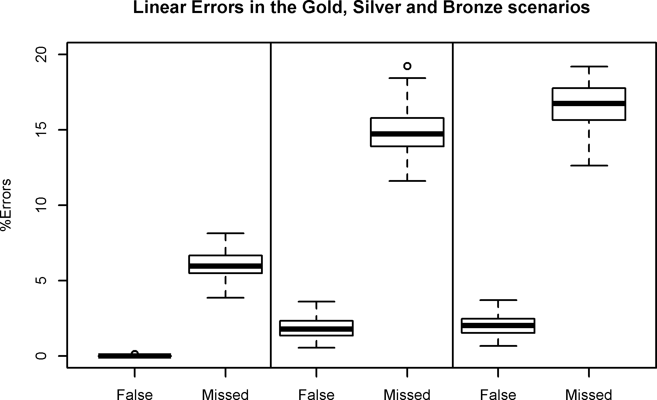
The error (1-λ) plays an important role in the adjustments. The use of the true values for (1-λ) and (1-α) instead of estimating them (e.g. via Eqs (2.1) and (3)) allows the comparison of the adjusted regression estimators against the naïve estimator without the effect of the linkage errors estimation. The distribution of the False Match Rate and the Missing Match Rate over the 100 replicates is represented in Fig. 1.

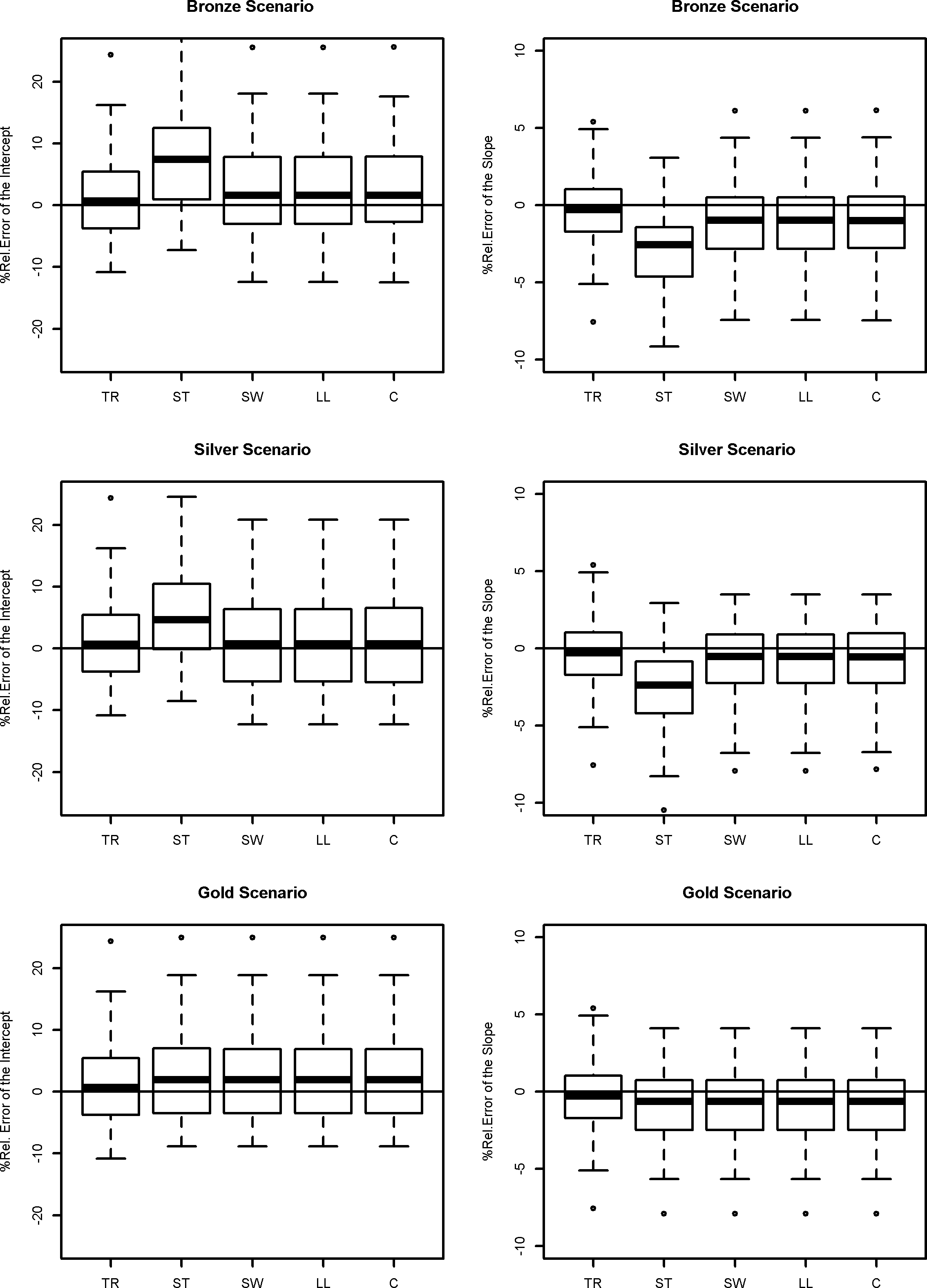
Figure 2.

Percentage of relative errors for true values, standard estimators and adjusted estimators in linear regression model.

The three scenarios produce increasing values of false and missing match rates. Primarily, the false match rate is under control, as in real practical applications where a conservative linkage strategy is often preferred; indeed, in our worst scenario the values of the false match rate are less than 5%. On the other hand, the control of the false match rate results in an increase of the missing match rate, which takes up to 20% in the Bronze Scenario.

However, under the standard assumption of ignorability of the missing linkage mechanism, one expects that the presence of missing matches does not introduce bias in the estimates even if it has an impact on their variability.

4.3Results

The following tables show the results of the previous estimators Eqs (4)–(7) for the linear model as well as of the standard estimator and the derived estimators from Eqs (9)–(11) for the logistic model.

As already mentioned in Section 3, the assumptions of the methods proposed in Chambers [11] are far to be met in practical situations. In our simulation, although different real contexts are reproduced, the exchangeability is assumed for the application of the adjusted estimators. Even if the assumption of exchangeability of linkage errors is not met even in sub-groups, only one block is considered and an overall value of the probability of correct match λ is applied for correcting the bias.

Table 2 reports the values of the linear regression model parameters and their relative standard errors for the naïve (4) and the adjusted estimators, SW (5), LL (6) and C (7), as well as the true values calculated on the whole population of 26450 records and the estimates obtained with the sample under perfect linkage.

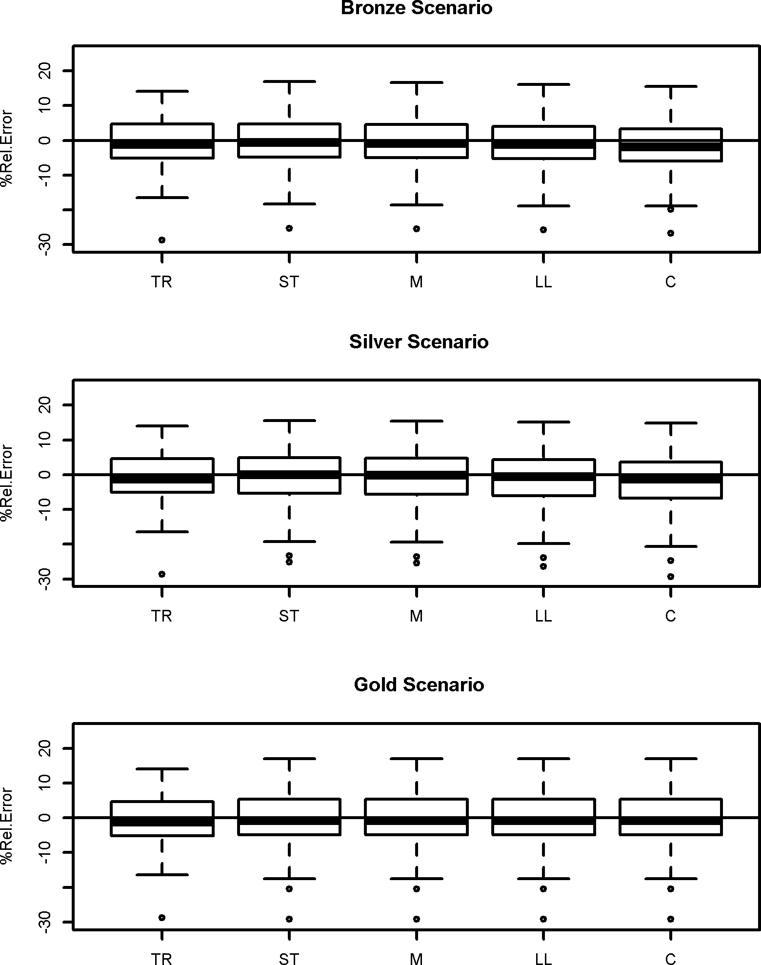
Figure 3.

Percentage of relative errors for true values, standard estimators and adjusted estimators in logistic regression model.

In Fig. 2, the percentage relative errors of the estimates under perfect linkage (TR), the naïve estimates in case of linkage errors (N) and the adjusted estimates in linear regression model are plotted.

As expected, the presence of false matches weakens the correlation between x and y in the linear regression model. Hence, the naïve estimator of the slope is increasingly biased towards 0, as the false linkage rate increases. On the contrary, the estimator of the intercept is biased in the opposite direction (if the mean value of the observed y, y* does not change). Even if the exchangeability assumption is not valid, the adjusted estimators provide bias reduction when the false match rate is not negligible with a limited increase in the variance compared to the naïve estimator.

The results of the logistic regression model are summarised in Table 3, where the parameter estimates and their relative standard errors are reported, averaging on 100 replicas. The table also shows the number of time the confidence intervals of the obtained estimates contains the true parameter value, i.e. the coverage of the nominal 95% CIs.

In Fig. 3 the distributions of relative errors of parameter estimates are plotted.

For categorical data, the false match error has less impact because of the nature of the response variable: the values of y and y* can be the same even when there is a linkage error and the conditional distribution (y*|x) may not differ appreciably from the conditional distribution (y|x). The results show that the bias of the naïve estimator of β does not increase noticeably from the Gold to the Bronze scenario. In this case, the correction does not reduce the bias of the standard estimator.

The results of the coverage evaluation show that the standard error evaluation might be severely affected by underestimation.

These results suggest that the missing matches should also be taken into account to completely remove the bias. Indeed, in the Gold scenario, where the false matches are close to zero, the naïve and the adjusted estimators are still biased due to a not-ignorable missing mechanism. The bias effect of the missing matches is also shown in the other scenarios, where the adjustments for false matches reduce the bias but do not eliminate it. In any case, the correction for the bias is more effective in the linear than in the logistic model: in linear regression, we achieve a bias reduction of about 10% for the Bronze scenario and a little smaller in the Silver one. However, more work is needed for the estimation of the logistic regression, where the naïve estimator is slightly closer to the benchmark value than the adjusted ones, but about 15% of the replicas produces values out of the nominal 95% CI.

As expected, the comparison of the standard errors of the estimator under perfect linkage and the naïve estimator shows that the occurrence of missed matches also produces an increase in variance due to the reduction of the observed sample size, similarly to a missing value mechanism.

References

[1] | Groves RM, Fowler FJ, Couper MP, Lepkowski JM, Singer E, Tourangeau R. Survey Methodology, 2nd Edition, Wiley (2004) . |
[2] | Bakker B. Micro-integration: State of the Art. Paper for the 2010 Joint UNECE/Eurostat Expert Group Meeting on Register-Based Censuses, The Hague, The Netherlands. |
[3] | Zhang L-C. Topics of statistical theory for register-based statistics and data integration. Statistica Neerlandica (2012) ; 66. |
[4] | Biemer P. Total survey error design, implementation, and evaluation. Public Opinion Quarterly (2010) ; 74: (5): 817-848. |
[5] | Fellegi IP, Sunter AB. A Theory for record linkage. Journal of the American Statistical Association (1969) ; 64: : 1183-1210. |
[6] | Jaro M. Advances in record linkage methodology as applied to matching the 1985 test census of Tampa, Florida. Journal of American Statistical Association (1989) ; 84: : 414-420. |
[7] | Neter J, Maynes ES, Ramanathan R. The effect of mismatching on the measurement of response error. Journal of the American Statistical Association (1965) ; 60: : 1005-1027. |
[8] | Scheuren F, Winkler WE. Regression analysis of data files that are computer matched – part I. Survey Methodology (1993) ; 19: : 39-58. |
[9] | Scheuren F, Winkler WE. Regression analysis of data files that are computer matched – part II. Survey Methodology (1997) ; 23: : 157-165. |
[10] | Lahiri P, Larsen M. Regression analysis with linked data. Journal of the American Statistical Association (2005) ; 100: : 222-230. |
[11] | Chambers R. Regression Analysis Of Probability-Linked Data. Official Statistics Research Series (2009) ; 4. |
[12] | Chambers R, Chipperfield J, Davis W, Kovacevic M. Inference Based on Estimating Equations and Probability-Linked Data. Centre for Statistical and Survey Methodology, University of Wollongong, Working Paper 18-09, (2009) . http://ro.uow.edu.au/cssmwp/38. |
[13] | Kim G, Chambers R. Regression analysis under incomplete linkage. Centre for Statistical and Survey Methodology, University of Wollongong, Working Paper 17-2009. |
[14] | Samart K. Analysis of probabilistically linked data. Doctor of Philosophy Thesis, School of Mathematics and Applied Statistics, University of Wollongong, (2011) . http://ro.uow.edu.au/theses/3513. |
[15] | Di Consiglio L, Tuoto T. Small Area Estimation in the Presence of Linkage Errors. In: Ferraro M. et al. (eds) Soft Methods for Data Science, Advances in Intelligent Systems and Computing Springer, Cham (2017) ; 456: . |
[16] | Briscolini D, Di Consiglio L, Liseo B, Tancredi A, Tuoto T. New methods for small area estimation with linkage uncertainty. International Journal of Approximate Reasoning (2018) ; 94: : 30-42. |
[17] | Chipperfield JO, Bishop GR, Campbell P. Maximum likelihood estimation for contingency tables and logistic regression with incorrectly linked data. Survey Methodology (2011) ; 37: (1): 13-24. |
[18] | Fortini M, Liseo B, Nuccitelli A, Scanu M. On Bayesian Record Linkage. Research in Official Statistics (2001) ; 1: : 185-198. |
[19] | Tancredi A, Liseo B. Some advances on Bayesian record linkage and inference for linked data, workshop Essnet DI, Madrid, November 2011. |
[20] | Steorts R, Hall R, Fienberg SE. A Bayesian approach to graphical record linkage and de-duplication. Journal of the American Statistical Association (2015) . URL: http://arxiv.org/abs/1312.4645. |
[21] | Winkler WE. Quality and analysis of national files – computational methods for censuses and surveys. Presentation, January 9, 2014. |
[22] | Essnet DI, McLeod P, Heasman D, Forbes I. Simulated data for the on the job training, (2011) . https://ec.europa.eu/eurostat/cros/content/job-training_en. |
[23] | RELAIS. User’s guide version 3.0, (2015) , available at https://joinup.ec.europa.eu/release/relais-30-0. |
[24] | Belin TR, Rubin DB. A method for calibrating false-match rates in record linkage. Journal of the American Statistical Association (1995) ; 90: : 694-707. |
[25] | Tuoto T. New proposal for linkage error estimation. Statistical Journal of the IAOS (2015) ; 32: (2). |