
Divide-and-Conquer solutions for estimating large consistent table sets1
Abstract
When several frequency tables need to be produced from multiple data sources, there is a risk of numerically inconsistent results. This means that different estimates are produced for the same cells or marginal totals in multiple tables. As inconsistencies of this kind are often not tolerated, there is a clear need for compilation methods for achieving numerically consistent output. Statistics Netherlands developed a Repeated Weighing (RW) method for this purpose. The scope of applicability of this method is however limited by several known estimation problems. This paper presents two new Divide-and-Conquer (D&C) methods, based on quadratic programming (QP) that avoid many of the problems experienced with RW.
1.Introduction
Statistical outputs are often interconnected. Different tables may share common cells or marginal totals. In such cases numerically consistency is often required, i.e. that the same values are published for common outputs. However, due to different data sources and compilation methods, numerically consistency is often not automatically achieved. Hence, there is a clear need for methods for achieving numerically consistent output.
An important example of a multiple table statistical output in the Netherlands is the Dutch Population and Housing Census. For the census, dozens of detailed contingency tables need to be produced with many overlapping variables. Numerically consistent results are required by the European Census acts and a number of implementing regulations [1]. In a traditional census, based on a complete enumeration of the population, consistency is automatically present. Statistics Netherlands belongs to a minority of countries that conducts a virtual census. In a virtual census estimates are produced from already available data that are not primary collected for the census. The Dutch virtual census is for a large part based on integral information from administrative sources. For a few variables not covered by integral data sources, supplemental sample survey information is used. Because of incomplete data, census compilation relies on estimation. Due to the different data sources that are used numerically inconsistent results would be inevitable if standard estimation techniques were applied [2, 3].
To prevent inconsistency, Statistics Netherlands developed a method called “Repeated Weighting” (RW), see e.g. [4, 5, 6, 7], a method that was applied to the 2001 and 2011 Censuses. In RW the problem of consistently estimating a number of contingency tables with overlapping variables is simplified by splitting the problem into dependent sub problems. In each of these sub problems a single table is estimated. Thus, a sequential estimation process is obtained.
The implementation of RW is however not without its problems (see [6, 8] and Subsection 2.4 below). In particular, there are problems that are directly related to the sequential approach. Most importantly, RW does not always succeed in estimating a consistent table set, even when it is clear that such a table set exists. After a certain number of tables have been estimated, it may become impossible to estimate a new one consistently with all previously estimated ones. This problem seriously limits future application possibilities of repeated weighting. For the Dutch 2011 Census several ad-hoc solutions were applied, designed after long trial-and-error. For any future application, it is however not guaranteed that numerically consistent estimates can be produced. Therefore, there is a clear need for extending methodology.
This paper presents two new ‘Divide-and-Conquer algorithms’ based on Quadratic Programming (QP). The algorithms break down the problem of consistent estimation of a set of contingency tables into sub problems that can be independently estimated, rather than the dependent parts that are obtained in RW. Thus, the estimation problems, as experienced with RW, are avoided.
In Section 2, we describe the RW method. Section 3 presents an alternative quadratic programming (QP) formulation for this problem. Section 4 gives a simultaneous weighting approach, which is the basis for the two new Divide-and-Conquer methods that are introduced in Section 5. Results of a practical application are given in Section 6 and finally Section 7 concludes this paper with a discussion.
2.Repeated weighting
In this section we explain the RW method. Subsection 2.1 describes prerequisites. The main properties of the method are given in Subsection 2.2. A more technical description follows in Subsection 2.3 and Subsection 2.4 presents known complications of the method.
2.1Prerequisites
Although RW can be applied to contingency and continuous data, this paper deals with contingency tables only.
I assume that multiple prescribed tables need to be produced with overlapping variables. If there were no overlapping variables, it would not be any challenge to produce numerically consistent estimates.
Further, it is assumed that the target populations are the same for each table. This means for example that all tables necessarily have to add up to the same grand-total.
All data sources relate to the same target population. There is no under- or overcoverage: the target population of the data sources coincides with the target population of the tables to be produced.
Further, for each target table a predetermined data set has to be available from which that table is compiled.
Two types of data sets will be distinguished: data sets that cover the entire target population and data sets that cover a subset of that population. As the first type is often obtained from (administrative) registers and the latter type from statistical sample surveys, these data sets will be called registers and sample surveys from now on.
It is assumed that all register-based data sets are already consistent at the beginning of RW. That means that all common units in different data sets have the same values for common variables. Subsection 2.2 explains why this assumption is important. In practise, this assumption often means that a so-called micro integration process has to be applied prior to repeated weighting [9].
For sample survey data sets it is required that weights are available for each unit that are meant to be used to draw inferences for a population. To obtain weights for sample surveys, one usually starts with the sample weight, i.e. the inverse of the probability of selecting a unit in the sample. Often, these sample weights are adjusted to take selectivity or non-response into account. Resulting weights will be called starting weights, as these are weights that are available at the beginning of repeated weighting.
2.2Non-technical description
The compilation method of a single table depends on the type of the underlying data set.
Tables that are derived from a register are simply produced by counting from that register. This means that for each cell in the table, it is counted how much the corresponding categories occur (e.g. 28 year old males). There is no estimation involved, because registers are supposed to cover the entire target population. The fact that register-based data are not adjusted explains why registers need to be already consistent at the beginning.
Below we focus on tables that are derived from a sample survey. These tables have to be consistently estimated. This basically means two things: common marginal totals in different tables have to be identically estimated and all marginal totals for which known register values exist have to be estimated consistently with those register values.
In the RW-approach consistent estimation of a table set is simplified by estimating tables in sequence. The main idea is that each table is estimated consistently with all previously estimated tables. When estimating a new table, it is determined first which marginal totals the table has in common with all registers and previously estimated tables. Then, the table is estimated, such that:
1) Marginal totals that have already been estimated before are kept fixed to their previously estimated values;
2) Marginal totals that are known from a register are fixed to their known value.
To illustrate this idea, we consider an example in which two tables are estimated:
Table 1: age
Table 1
Marginal total 1
| Citizenship | Education | Count |
|---|---|---|
| Oceania | Low | 1 |
| Oceania | High | 9 |
Table 2
Marginal total 2
| Industry | Education | Count |
|---|---|---|
| Mining | Low | 49 |
| Mining | High | 2 |
A register is available that contains age, sex and geographic area. Educational attainment is available from a sample survey. Because educational attainment appears in Tables 1 and 2, both tables need to be estimated from that sample survey. To achieve consistency, Table 1 has to be estimated, such that its marginal totals age
Each table is estimated by means of the generalised regression estimator (GREG) [10], an estimator that belongs to the class of calibration estimators [11]. Thus, repeated weighting comes down to a repeated application of the GREG-estimator.
2.3Technical description
In this subsection, repeated weighting is described in a more formal way. Below we will explain how a single table is estimated from a sample survey.
Aim of the repeated weighting estimator (RW-estimator) is to estimate the
A simple population estimator is given by
where
The so-called initial table estimate
There is a relationship between the cells of a table and its marginal totals: a marginal total is a collapsed table that is obtained by summing along one or more dimensions. Each cell contributes to a specific marginal total or it does not. The relation between the
A table estimate
(1)
Usually, initial estimates
Therefore, our aim is to find a table estimate
(2)
such that:
where
Despite that several alternative methods can be applied as well, e.g. [11, 12], the Generalised Least Squares (GLS) problem in Eq. (2) has a long and solid tradition in official statistics.
A closed-form expression for the solution of the problem in Eq. (2) can be obtained by the Lagrange Multiplier method (see e.g. [13]). This expression is given by
(3)
The GREG-estimator is obtained as special case of Eq. (3) in which
(4)
In writing Eq. (4), it is assumed that the inverse of square matrix
As an alternative to minimizing adjustment at cell level, the RW solution can also be obtained by minimal adjustment of underlying weights. In [11] it is shown that a set of adjusted weights
(5)
For data sets that underlie estimates for multiple tables, adjusted weights are usually different for each table.
From the expression for the RW-estimator in Eq. (4), it follows that initial cell estimates of zero remain zero, since the relevant rows in
Besides reconciled table estimates, RW also provides means to estimate precision of these estimates. Variances of table estimates can be estimated, see [6] for mathematical expressions.
2.4Problems with repeated weighting
Below we summarise complications of RW. Problems that are inherent to the sequential way of estimation are described first, then other complications are given.
2.4.1Problem 1. Impossibility of consistent estimation
A first problem of RW is that, after a number of tables have been estimated, it may become impossible to estimate a new one. Earlier estimated tables impose certain consistency constraints on a new table, which reduces the degree of freedom for the estimation of that new table. When a number of tables have already been estimated it may become impossible to satisfy all consistency constraints at the same time. The problem is also known in literature [15], for the estimation of multi-dimensional tables with known marginal totals.
Example
Suppose one wants to estimate the table country of citizenship
By combining both tables it can be seen that the combination Oceania & mining industry can occur three times at most; there cannot be more than two highly educated people and one lowly educated person. This contradicts results from the register that states that there are four “mining” persons from Oceania. The problem occurs because the known population counts for the combination of citizenship and industry are not taken into account in the previously estimated tables.
2.4.2Problem 2. Suboptimal solution
In the RW-approach the problem of estimating a set of coherent tables is split into a number of sub problems, in each of which one table is estimated. Because of the sequential approach, a suboptimal solution may be obtained that deviates more from the data sources than necessary.
2.4.3Problem 3. Order dependency
The order of estimation of the different tables matters for the outcomes. Besides that ambiguous results are not desirable as such, it can be expected that there is a relationship between the quality of the RW-estimates and the order of estimation, as tables that are estimated at the beginning of the process do not have to satisfy as many consistency constraints as tables that are estimated later in the process.
In addition to the aforementioned problems, there are also some other problems that are not directly caused by sequential estimation.
A first problem is that although RW achieves consistency between estimates for the same variable in different tables, the method does not support consistency rules between different variables (so-called ‘edit rules’). An example of such a rule is that the number of people who have never resided abroad cannot exceed the number of people born in the country concerned.
A second complication is that RW may yield negative cell estimates. In many practical applications, such as the Dutch Census, negative values are however not allowed.
A third complication is the previously mentioned empty cell problem. As mentioned in Subsection 2.3, this problem occurs when estimates have to be made without underlying data. It is caused by sampling effects, i.e. characteristics that are known to exist in the population that are not covered by a sample survey used for estimation. The empty cell problem can be tackled by the epsilon method: a technical solution [16] based on the pseudo-Bayes estimator [17] for log-linear analysis. The epsilon method means that zero-valued estimates in an initial table are replaced by small, artificial, non-zero “ghost” values, which were set to one for all empty cells in the 2011 Census tables. In other words, it was assumed a priori that each empty cell is populated by one fictitious person.
3.Repeated weighting as a QP problem
This section demonstrates that the consistent estimation problem can alternatively be solved by available techniques from Operations Research (OR). The repeated weighting estimator in Eq. (4) can be obtained as a solution of the following quadratic programming problem (QP).
(6)
such that:
The objective function minimizes squared differences between reconciled and initial estimates. The constraints are the same as in RW. The last mentioned type of constraint ensures that zero-valued estimates are not adjusted.
The main advantage of the QP-approach is its computational efficiency. Unlike the closed-form expression of the RW estimator Eq. (4), Operations Research methods do not rely on matrix inversion. Therefore, very efficient solution methods are available (e.g. [18]). Operations Research methods are available in efficient software implementations (‘solvers’), that are able to deal with large problems. Examples of well-known commercial solvers are Xpress, Gurobi and Cplex [19, 20, 21]. In the Netherlands, mathematical optimization methods are applied for National Accounts balancing [22]; an application that requires solving a quadratic optimization problem of approximately 500,000 variables.
A second advantage of the QP-approach is that it can still be used in case of redundant constraints. Contrary to the WLS-approach, there is no need to remove redundant constraints, or to apply sophisticated techniques like generalised inverses.
A third advantage is that QP can be more easily generalised than WLS to include additional requirements. Inequality constraints can be included in the model to take account of non-negativity requirements and edit rules (see Subsection 2.4). The empty cell problem can be dealt with by the following slight modification of the objective function
(7)
such that:
where
Disadvantages of the QP-approach are that the method does not provide means to derive corrected weights and to estimate variances of reconciled tables. However, because of the equivalence of the QP and the WLS formulation of the problem, it follows that, although corrected weights are not obtained in a solution of a QP-problem, these weights do exist from a theoretical point of view.
4.Simultaneous approach
In this section we argue that the three problems mentioned in Subsection 2.4 (“Impossibility of consistent estimation”, “Suboptimal solution” and “Order dependency”) that are inherent to the sequential way of estimation can be circumvented in an approach in which all tables are estimated simultaneously. The QP-model in Eq. (6) can be easily generalized for the consistent estimation of a table set. That is, a consistent table set can be obtained as a solution to the following problem
(8)
such that:
In this formulation
The objective function minimises a weighted sum of squared differences between initial and reconciled cell estimates for all tables. The constraints impose marginal totals of estimated tables to be consistent with known population totals from registers and estimated tables to be mutually consistent. The former means that for each table all marginal totals with known register totals are consistently estimated with those register totals. The latter means that for each pair of two distinct tables all common marginal totals have the same estimated counts. These constraints impose a sum of cells in one table to be equal to a sum of cells in another table, where the value of that sum is not known in advance. For comparison, in RW, marginal totals of one table need to have the same value as known marginal totals from earlier estimated tables. Analogous to the RW-model in Eq. (6), the SW-model in Eq. (8) can be easily extended to take account of additional requirements, like non-negativity of estimated cell values, edit rules and the empty cell problem.
It can be easily seen that Problems 1, 2 and 3 in Subsection 2.4 do not occur if all tables are estimated simultaneously. Furthermore, from a practical point it is more attractive to solve one problem rather than several problems.
A SW-approach may however not always be computationally feasible. A large estimation problem needs to be solved consisting of many variables and constraints. The capability of solving such large problems may still be limited by computer memory size, even for modern computers. We therefore focus on ways of splitting the problem up into a number of smaller sub problems that can be preferably independently solved.
5.Divide-and-Conquer algorithms
In this section two so-called Divide-and-Conquer (D&C) algorithms are presented for estimating a set of coherent frequency tables. These algorithms recursively break down a problem into sub problems that can each be more easily solved than the original problem. The solution of the original problem is obtained by combining the sub problem solutions.
5.1Splitting by common variables
The main idea of our first algorithm is that an estimation problem, with one or more common register variable(s) can be split into a number of independent sub problems, based on the categories of these register variable(s). For example, if sex were included in all tables of a table set, a table set can be split into two independent sets: one for men and one for women.
In practice, it is often not the case that a table set has one or more common register variables in each table. Common variables can however always be created by adding variables to tables, provided that a data source is available from which the resulting, extended tables can be estimated. In our previous example, all tables that do not include sex can be extended by adding this variable to the table. In this way, the level of detail increases, meaning that more cells need to be estimated as in the original problem, which may come along with a loss of precision at the required level of publication. However, at the same time, the possibility is created of splitting a problem into independent sub problems. Since all ‘added’ variables are used to split the problem, one can easily understand that the number of cells in each of these sub problems cannot exceed the total number of cells of the original problem.
For any practical application the question arises which variable(s) should be chosen as “splitting” variable(s). Preferably, this/these should be variable(s) that appear in most tables, e.g. sex and age in the Dutch 2011 Census, as this choice leads to the smallest total number of cells to be estimated.
The approach is especially useful for a table set with many common variables, because in that case the number of added cells remains relatively limited.
The proposed algorithm has the advantage over Repeated Weighting that the sub problems that are created can be solved independently. For this reason there are no problems with “impossibility of estimation” (Problem 1 in Subsection 2.4) and “order-dependency of estimation” (Problem 3 in Subsection 2.4). Problem 2 “suboptimal solution” is not necessarily solved. This depends on the need of adding additional variables to create common variables. If a table set contains common register variables in each table and the estimation problem is split using these common variables, an optimal solution is obtained. However, if common variables are created by adding variables to tables, extended tables are obtained, for which the optimal estimates do not necessarily comply with the optimal estimates for the original tables.
5.2Aggregation and disaggregation
A second divide-and-conquer algorithm consists of creating sub problems by aggregation of one or multiple variable categories. In the first stage, categories are aggregated (e.g. estimating ‘educational attainment’ according to two categories rather than the required eight). In a second stage, table estimates that include the aggregation variable(s) are further specified according to the required definition of categories.
Since the disaggregation into required categories can be carried out independently for each aggregated category, a set of independent estimation problems is obtained in the second stage.
For example, suppose that we need to estimate educational attainment, according to 8 categories: 1,
In the previous example one variable was aggregated, educational attainment. It is however also possible to aggregate multiple variables. In that case a multi-step method is obtained, in which in each stage after Stage 1, one of the variables is disaggregated.
Because of these dependencies of the estimation processes in different stages, it cannot be excluded that the three problems of Section 2.5 occur. However, the problems are likely to have a lower impact than in RW. This is because of a lower degree of dependency: in RW each estimated table may be dependent on all earlier estimated tables, whereas in the proposed D&C approach, estimation of a certain sub problem only depends on one previously solved problem.
6.Application to Dutch 2011 Census
In this section we present results of a practical application of the proposed Divide-and-conquer (D&C) methods to the Dutch 2011 Census tables. Our aim is to test the feasibility of the methods, as well as to compare results with the officially published results that are largely based on RW. Subsection 6.1 describes backgrounds of the Dutch Census. Subsection 6.2 explains the setup of the tests and Subsection 6.3 discusses results.
6.1Dutch 2011 Census
According to the European Census implementing regulations, Statistics Netherlands was required to compile sixty high-dimensional tables for the Dutch 2011 Census, for example, the frequency distribution of the Dutch population by age, sex, marital status, occupation, country of birth and nationality. Since the sixty tables contain many common variables ‘standard weighting’ does not lead to consistent results.
Several data sources are used for the Census, but after micro-integration, two combined data sources are obtained: one based on a combination of registers and the other one is a combination of sample surveys [23]. From now on, when we refer to a Census data source, a combined data source is meant after micro-integration. The ‘register’ data cover the full population (in 2011 over 16.6 million persons) and include all relevant Census variables except ‘educational attainment’ and ‘occupation’. For the ‘sample survey’ data it is the other way around, these data cover all relevant Census variables, but it is available for a subset of 331,968 persons only.
For the 2011 Census 42 tables needed to be estimated that include ‘educational attainment’ and/or ‘occupation’. The target population of these tables consists of the registered Dutch population, with the exception of people younger than 15 years. Young children are excluded because the two sample survey variables ‘educational attainment’ and ‘occupation’ are not relevant for these people.
The total number of cells in the 42 tables amounts to 1,047,584, the number of cells within each table ranges from 2,688 to 69,984.
6.2Setup
Below we explain how the two D&C algorithms were applied to the 2011 Dutch Census.
6.2.1Setup 1 – Splitting by common variables
In this setup, the original table set is split into 48 independently estimated table sets, by using geographic area (12 categories), sex (2 categories), and employment status (2 categories) as splitting variables. Each of the 48 table sets contains a subset of the 42 Census tables, determined by the categories of the splitting variables.
The three splitting variables are however not present in all 42 Census tables. In 13 tables geographic area is missing and in one table sex is absent. Tables that do not include the three splitting variables were extended by incorporating missing variables. As a result, the total number of cells in the 42 tables was increased from 1,047,584 to 4,556,544.
6.2.2Setup 2 – Aggregation and disaggregation
In this setup educational attainment (8 categories) and occupation (12 categories) were selected for aggregation of categories. Initially, both variables are aggregated into two main categories, that each contain half of the categories of the original variables. Thereafter, results were obtained for the required categories for the two aggregation variables.
Five optimization problems are defined in this procedure. In the first problem a table set is estimated based on aggregated categories for educational attainment and occupation. In each of the following stages either one of the two aggregated categories for educational attainment or occupation is disaggregated into required categories. Since less sub problems are defined, it follows that average problem size is larger than for Setup 1.
6.3Results
In this subsection we compare results of the two D&C methods with the RW-based method as applied to the official 2011 Census. All practical tests were conducted on a 2.8 GHZ computer with 3.00 GB of RAM. Xpress was used as solver [19].
A simultaneous estimation of the required 42 Census tables, as described in Section 4, turned out to be infeasible, due to memory problems of the computer.
The two D&C approaches were however successfully applied; there were no problems from a technical perspective and the estimation problems as experienced with RW were avoided.
Thus, we arrive at our main conclusion that the D&C approaches have broader applicability than RW.
We now continue with a comparison of the reconciliation adjustments. The criterion used to compare degree of reconciliation adjustment is based on the QP objective function in Eq. (7), a sum of weighted squared differences between initial and reconciled estimates, given by
(9)
where
Table 3 compares total adjustment, as defined according to Eq. (9), based on all cells in all 42 estimated tables.
Table 3
Total adjustment; three methods
| Method | Total adjustment (*10 | |
|---|---|---|
| All cells | Cells with initial estimate | |
| larger than zero | ||
| Dutch 2011 Census | 109.64 | 12.68 |
| Splitting by common variables | 88.35 | 12.37 |
| Aggregation and disaggregation | 69.56 | 12.47 |
Figure 1.
Boxplots of adjustments to all cells of 42 Census tables. The right panel zooms in on the lower part of the left panel.
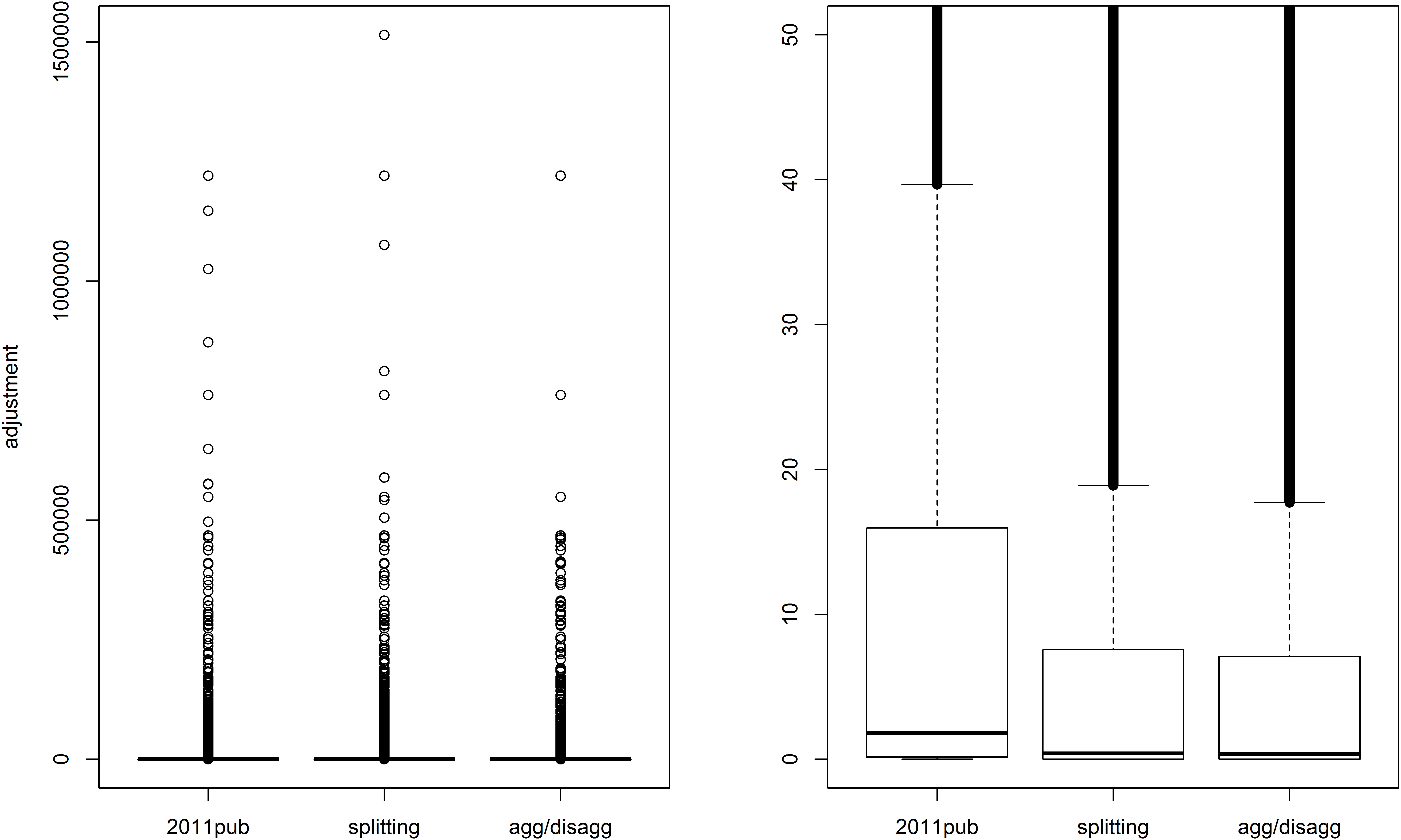
The two newly developed D&C methods lead to smaller total adjustment than RW.
The result that “Aggregation and Disaggregation” method gives rise to a better solution than “Splitting by common variables” can be explained by the lower amount of sub-problems that are defined in the chosen setups.
However, if we only compare cells with larger than zero initial estimates, differences between three methods become very small. This shows that the way how original estimates of zero are processed is more important than the way how the estimation problem is broken down into sub problems.
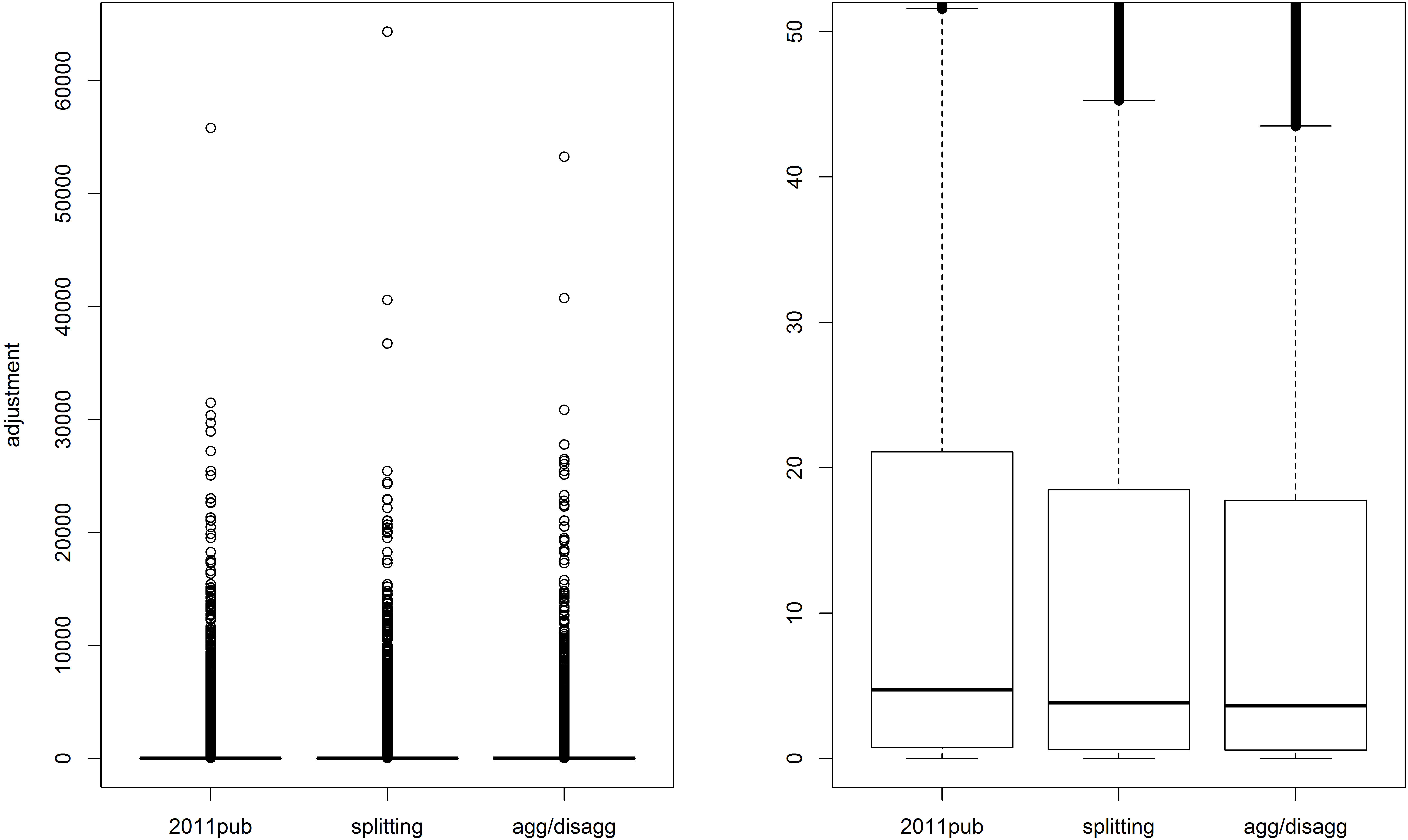
The boxplots in Figs 1 and 2 compare adjustment at the level of individual cells. It can be seen that the amount of relatively small corrections is larger for the two D&C methods than for the RW-based method used for officially published Census tables. Differences in results are however smaller again, if zero initial estimates are not taken into account.
Figure 2.
Boxplots of adjustments to all cells with nonzero initial estimates. The right panel zooms in on the lower part of the left panel.
7.Discussion
When several frequency tables need to be produced from multiple data sources, the problem may arise that results are numerically inconsistent. That is, that different results are obtained for the same marginal totals in different tables. To solve this problem, Statistics Netherlands developed a Repeated Weighting (RW) method. This method was applied to the 2001 and 2011 Dutch censuses. However, the scope of applicability of this method is limited by several known estimation problems. In particular, the sequential way of estimation causes problems. As a result of these problems, estimation of the 2011 Census was troublesome. A suitable order of estimation was found after long trial and error.
This paper presented two alternative Divide and Conquer (D&C) methods that break down the estimation problem as much as possible into independently estimated parts, rather than the dependent parts that are distinguished in RW. One of the two newly developed methods partitions a given table set according to common categories of variables that are contained in each table. The other method is based on aggregation and disaggregation of categories.
As a result of independent estimation, many of the estimation problems of RW can be prevented. This greatly enhances the practicability of the method. Another advantage is that the reduced order-dependency of results leads to less ambiguity. A final advantage is that the new approaches can be more easily extended to incorporate additional requirements, like non-negativity of estimates and solutions for the empty cell problem.
An application to 2011 Census tables showed that estimation problems were actually avoided. Reconciliation adjustments were observed to be smaller than in RW. Hence, it can be argued that a better solution can be obtained that deviates less from the data sources. The smaller adjustments can be mainly attributed to the solution applied to the empty cell problem; a solution that could not be implemented in the original RW approach.
Hence, the key message of this paper is when estimating a consistent set of tables, there can be smarter ways of breaking down the problem than estimating single tables in sequence.
For problems in which a simultaneous estimation of all tables is computationally feasible, such an approach is to be preferred. Most importantly, because a full simultaneous approach avoids the estimation problems that are experienced with RW. Moreover, an optimal solution is obtained with minimal adjustment from the data sources. Finally, from a practical point of view solving one (or few) optimization problem(s) is much easier than solving many problems.
Acknowledgments
This author is grateful for the funding by the European Union that made this project possible. The author thanks Ton de Waal, Tommaso di Fonzo, Nino Mushkudiani, Eric Schulte Nordholt, Frank Linder, Arnout van Delden and Reinier Bikker for useful suggestions.
References
[1] | European Commission. Regulation (EC) No 763/2008 of the European Parliament and of the Council of 9 July 2008 on population and housing censuses. Official Journal of the European Union. (2008) ; L218: : 14-20. |
[2] | De Waal T. General Approaches for Consistent Estimation based on Administrative Data and Surveys [Internet]. The Hague: Statistics Netherlands; 2015; [cited 2017 Mar 24]. Available from: https//www.cbs.nl/-/media/imported/documents/2015/37/2015-general-approaches-to-combining-administrative-data-and-surveys.pdf. |
[3] | Waal T. Obtaining numerically consistent estimates from a mix of administrative data and surveys. Statistical Journal of the IAOS. (2016) ; 32: : 231-43. doi: 103233/SJI-150950. |
[4] | Renssen RH, Nieuwenbroek NJ. Aligning Estimates for Common Variables in two or more Sample Surveys. Journal of the American Statistical Association. (1997) ; 90: : 368-74. |
[5] | Nieuwenbroek NJ, Renssen RH, Hofman L. Towards a generalized weighting system. In: Proceedings, Second International Conference on Establishment Surveys, Alexandria VA: American Statistical Association; (2000) . p. 667-76. |
[6] | Houbiers M, Knottnerus P, Kroese AH, Renssen RH, Snijders V. Estimating Consistent Table Sets: Position Paper on Repeated Weighting. The Hague: Statistics Netherlands; (2003) ; [cited 2017 Mar 24]. Available from: https//www.cbs.nl/-/media/imported/documents/2003/31/discussion-paper-03005.pdf. |
[7] | Knottnerus P, Duin van C. Variances in Repeated Weighting with an Application to the Dutch Labour Force Survey. Journal of Official Statistics. (2006) ; 22: : 565--84. |
[8] | Daalmans J. Estimating Detailed Frequency Tables from Registers and Sample Surveys. The Hague: Statistics Netherlands; (2015) ; [cited 2017 Mar 24]. Available from: https//www.cbs.nl/-/media/imported/documents/2015/07/201503dp-estimating-detailed-frequency-tables-from-registers-and-sample-surveys.pdf. |
[9] | Bakker BFM, Rooijen van J, Toor van L. The system of social statistical datasets of Statistics Netherlands: an integral approach to the production of register-based social statistics. Statistical journal of the IAOS. (2014) ; 30: : 411-24. doi: 103233./SJI-140803. |
[10] | Särndal CE, Swensson B, Wretman J. Model assisted survey sampling, New York: Springer Verlag; (1992) . |
[11] | Deville JC, Särndal CE. Calibration Estimators in Survey Sampling. Journal of the American Statistical Association. (1992) ; 87: : 376-82. |
[12] | Little RJA, Wu M. Models for Contingency Tables with known margins when Target and Sampled Populations Differ. Journal of the American Statistical Association. (1991) ; 86: : 87-95. |
[13] | Mushkudiani N, Daalmans J and Pannekoek J. Reconciliation of labour market statistics using macro-integration. Statistical Journal of the IAOS. (2015) ; 31: : 257-62. |
[14] | Ben-Israel A, Greville TNE. Generalized inverses Theory and applications. 2 |
[15] | Cox LH. On properties of multi-dimensional statistical tables. Journal of Statistical Planning and Inference. (2003) ; 117: : 251-73. |
[16] | Houbiers M. Towards a Social Statistical Database and Unified Estimates at Statistics Netherlands. Journal of Official Statistics. (2004) ; 20: : 55-75. |
[17] | Bishop Y, Fienberg S, Holland P. Discrete Multivariate Analysis: Theory and Practice. Cambridge: MIT Press; (1975) . |
[18] | Nocedal J, Wright SJ. Numerical Optimization, 2 |
[19] | Dash Optimization, Xpress-Optimizer Reference manual, Warwickshire: Dash Optimization; (2017) . |
[20] | IBM, ILOG CPLEX V 126. User’s Manual for CPLEX. IBM Corp.; (2015) . |
[21] | Gurobi, Gurobi Optimizer Reference Manual, Houston: Gurobi Optimization Inc; (2016) . |
[22] | Bikker RP, Daalmans J, Mushkudiani N. Benchmarking Large Accounting Frameworks: A Generalised Multivariate Model Economic. Systems Research (2013) ; 25: ; 390-408. doi: 101080/09535314.2013.801010. |
[23] | Schulte Nordholt E, Zeijl van J, Hoeksma L. The Dutch Census 2011: analysis and methodology, The Hague: Statistics Netherlands; (2014) [cited 2017 Mar 24]. Available from https//www.cbs.nl/NR/rdonlyres/5FDCE1B4-0654-45DA-8D7E-807A0213DE66/0/2014b57pub.pdf. |


