
The value added and operating surplus deflators for industries: The right price indicators that should be used to calculate the real interest rates
Abstract
After the global financial crisis of 2008–2009, many advanced economies are suffering from a dearth of domestic investment opportunities. It has been said that lowering real interest rate is the best policy to boost the capital investment. The problem is what inflation rate they have in their mind when the entrepreneurs make investment decisions. Not only the output prices, but also the composition of inputs differ from one industry to another. Therefore, the value added deflator or even the operating surplus deflator for each industry are better alternative to calculate the real interest rate. In the first half of the paper, we examine the theoretical meaning of the value added deflators using a highly simplified symmetric input output table. In the latter half, we will use so-called SNA-IO, the input-output table published as a part of Japanese SNA, to experimentally estimate both value added and operating surplus deflators. The study reveals that if lowering interest rate depreciate the local currency, it will depress value added deflators, and in turn, will discourage capital investments. In this sense, lowering interest rate is a double-edged sword; the governments and central banks should think twice before taking such a policy.
1.Introduction
With slowly growing or declining workforces, as well as high capital-labor ratios, many advanced econ-omies face an apparent dearth of domestic investment opportunities, while the ageing society calls for more savings (i.e. future consumption) to prepare for the retirement (Bernanke [1]). Traditionally, it was thought that if you wanted to boost the capital investment, the central bank would reduce interest rates. Wicksell [2] (Chapters VIII and IX) defined natural rate of interest (natürliche Kapitalzins) as the physical rate of return on capital investment at the time. If the market rate of interest on loans (Darlehnszins) is below the natural rate, entrepreneurs will borrow funds and make profit by investing in capital goods. On the contrary, if the market rate is above the natural rate, the entrepreneurs will be hesitant to borrow so that capital investment will stagnate. However, Wicksell also asserted that, even in such a situation, the entrepreneurs are willing to invest if they face an inflation because it will increase the monetary return. Therefore, he concluded that capital investment will increase as the real rate of interest, which is market rate of interest less the rate of inflation, declines. The problem is what inflation rate they have in their mind when the entrepreneurs make investment decisions.
A price index is a measure of the proportionate, or percentage, changes in a set of prices over time; usually it consists of per-unit transaction value of specific product (prices) and some indicator of the proportionate composition of the products (share weight) among the group of products in question. For example, a consumer price index (CPI) measures changes in the prices of goods and services that households consume (ILO [3]). In an analogy, so called producer price index (PPI) measures changes in the prices of goods and services that domestic producers produce. However, as IMF [4] asserts, the producers are at the same time purchasers of goods and services because they consume other producers’ outputs as intermediate inputs – materials, components, fuels, etc. The value added deflator is a price indicator that takes this two-sidedness of the producers; it is defined as the proportion of the nominal value added to the real value added, which is obtainable by dividing both the output and the intermediate inputs in nominal terms by the appropriate price indices.11 The remaining problem is that the value added deflator does not take the wage rate and other production factor cost into consideration; in this context, it is desirable to obtain the operating surplus deflator rather than the value added deflator. This paper discusses the issues concerning the measurement of the deflators for both value added and operating surplus for each industry.
After the tradition of the SNA 1968 (paragraphs 8.44 through 8.47) and 1993 (15.162 through 15.164), the SNA 2008 discusses value added deflator in paragraphs 14.153 through 14.157; it is defined using double deflation method22 in the framework of the supply and use tables. The proportion of the domestic total of nominal value added to that of real value added is casually referred to as GDP deflator (SNA 2008, 15.235); not a few statistical authorities publish it as a part of GDP statistics. Simple mathematics tells us that, as shown in Eq. (2.2) below, the GDP deflator is the weighted harmonic mean of the value added deflators. However, the meaning of the value added deflator for each industry is far more complicated because the weight for one particular item involves the prices of other items.
Table 1
Symmetric use table at current prices
| Industries (production activities) | Domestic | Exports | Imports | Total domestic output | ||||||
| 1 |
|
|
|
| final uses | |||||
| Products | 1 |
|
|
|
|
|
|
|
|
|
|
|
|
|
|
|
|
|
|
|
| |
|
|
|
|
|
|
|
|
|
|
| |
|
|
|
|
|
|
|
|
|
|
| |
|
|
|
|
|
|
|
|
|
|
| |
| Value | Added |
|
|
|
|
| ||||
| Total | Output |
|
|
|
|
| ||||
Table 2
Symmetric use table presented in constant prices
| Industries (production activities) | Domestic | Exports | Imports | Total | ||||||
| 1 |
|
|
|
| final uses | domestic output | ||||
| Products | 1 |
|
|
|
|
|
|
|
|
|
|
|
|
|
|
|
|
|
|
|
| |
|
|
|
|
|
|
|
|
|
|
| |
|
|
|
|
|
|
|
|
|
|
| |
|
|
|
|
|
|
|
|
|
|
| |
| Value | Added |
|
|
|
|
| ||||
| Total | Output |
|
|
|
|
| ||||
In addition to the value added deflator, the SNA 2008 mentions the operating surplus deflator in 14.157. In the framework of the generation of income account, the value added consists of three major components: compensation of employees, taxes/subsidies on production and imports, and gross operating surplus/mixed income. As paragraph 14.155 asserts, calculating compensation of employees in volume terms is possible if enough information is available on wage rates and numbers employed by category of worker. If it is possible, it is an easy task to obtain the deflator for compensation of employees. However, it seems far more difficult to know the taxes less subsidies on production in volume terms. To obtain the deflator for gross operating surplus, we have to overcome this critical problem. Despite all the difficulties, we tentatively obtained the deflator for gross operating surplus / mixed income for the Japanese industries to find out further problems we may encounter in practice.
2.Value added deflator
2.1Definitions
Before going into the empirical evidence, we examine the theoretical meaning of the value added deflators using a highly simplified use table in which one industry produces only one product so that the table reduces to a symmetric input output table as shown in Table 1 in current values (i.e. VAT inclusive). Note that paragraph 5.2 of SNA 2008 basically defines industry as a group of establishments engaged in the same production activity. Let subscripts
Let
(1)
where
(2)
The balance at constant price is as follows:
(3)
The above assumption tells us that the domestic and imported products are supplied to the domestic users at a price, which is the quantity-weighted average of the domestic and import prices:
(4)
Therefore
(5)
and
(6)
The input deflator for product
(7)
Likewise, the input deflator for all domestic products as a composite commodity is obtainable:
(8)
The output deflator for product
(9)
Furthermore, by assuming
(10)
As we have described already, in this model, gross value added for product
(11)
By summing up the above equation over
(12)
The above equation proves that GDP is equivalent to the sum of domestic final uses and exports less imports so that GDP can be obtained either in the production approach by summing up value added or in the expenditure approach using the latter relations. We further define real value added for product
(13)
By summing up the above equation over
(14)
According to the traditional double deflation method, as described in Paragraph 15.162 of the SNA 1993, the value added deflator for product
(15)
Likewise, we define GDP deflator as the ratio of nominal GDP to real GDP:
(16)
Therefore, in most cases, the expenditure approach is a more convenient way to get real GDP and the GDP deflator.
2.2Decompositions
The value added deflator for product
(17)
The last line of the above equation shows that the value added deflator for product
(18)
so that output price is a weighted average of the input prices and the value added deflator. Alternatively, we can decompose the value added deflator for product
(19)
The last line of the above equation tells us that the value added deflator for product
(20)
we can safely conclude that the effects of import prices on the value added deflator is negative.
Likewise, the GDP deflator (for all the domestic products as a composite commodity) could be decomposed in the following manner from Eq. (16) by substituting Eq. (4):
(21)
In other words, the GDP deflator consists of two portions: (i) that depends on the domestic factors, and (ii) that depends on the import prices. It should be noted that, since
(22)
the effects of import prices are inevitably negative.
Alternatively, we can decompose the GDP deflator into consisting products:
(23)
It means that the GDP deflator is a constant-price value-added weighted average of the value added deflator of each product. The problem of the above equation is that
(24)
In other words, the GDP deflator is simply regarded as a weighted harmonic mean of the value added deflators.
3.Operating surplus deflator
According to paragraphs 1.17 and 7.5 through 7.9 of SNA 2008, there are two main types of charges that producers have to meet out of gross value added: compensation of employees payable to workers employed and any taxes payable less subsidies receivable in the production process. Compensation of employees is defined as the total remuneration payable by an enterprise to an employee in return for work done by the latter. Taxes less subsidies on production consist of taxes payable or subsidies receivable (if negative) on goods or services produced as outputs, and other taxes or subsidies (if negative) on production. After deducting compensation of employees and taxes, less subsidies, on production from value added, the balancing item is obtained. The balancing item is described as gross operating surplus except for unincorporated enterprises owned by households in which the owner or members of the same household may contribute unpaid labor inputs of a similar kind to those that could be provided by paid employees. In the latter case, the balancing item is described as mixed income because it implicitly contains an element of remuneration for work done by the owner, or other members of the household, that cannot be separately identified from the return to the owner as entrepreneur.
As we have mentioned above, operating surplus
(25)
As paragraph 14.155 of SNA 2008 asserts, calculating compensation of employees in volume terms is possible if enough information is available on wage rates. Let us assume for simplicity that we can observe the wage rate for each industry
(26)
As United Nations [11] remarks, there are two types of taxes on production: ad valorem and non ad valorem; the former is levied as a percentage of the value of goods or services, but the latter is not.44 Since, in many countries, value-added type tax accounts most of the taxes on products, it must be plausible to define the price of it in reference to the real value added as follows because the VAT payable is the product of the value added before tax and the VAT rate:
(27)
We assume here, as a first approximation, that the other taxes on production relate to the output rather than the value added so that we tentatively define its price as:
(28)
We will normalize
(29)
We further define operating surplus at constant prices in the following manner:
(30)
The operating surplus deflator is defined as follows in analogy to the value added deflator:
(31)
4.Estimation of the deflators using Japanese SNA data
4.1Value added and operating surplus deflators
We will use so-called SNA-IO,55 the input-output table published as a part of Japanese SNA, to experimentally estimate both value added and operating
Table 3
Correlation coefficients between value added and related deflators (2001–2013)
| Correlation coefficients between | Correlation coefficients between | ||
| total output and value added deflators | input and value added deflators | ||
| 1 | Agriculture, forestry and fishing | 0.5939 | |
| 2 | Mining | 0.9181 | 0.3655 |
| 3 | Foods and beverages | 0.8310 | 0.3621 |
| 4 | Textiles | 0.8764 | 0.5018 |
| 5 | Pulp and paper products | 0.9705 | 0.7739 |
| 6 | Chemical products | 0.9651 | 0.9202 |
| 7 | Petroleum and coal products | 0.6595 | 0.5507 |
| 8 | Quarrying and pottery | ||
| 9 | Primary metals | 0.9558 | 0.9283 |
| 10 | Fabricated metal products | ||
| 11 | General machinery | 0.6308 | |
| 12 | Electric machinery and equipment | 0.9697 | 0.9021 |
| 13 | Transportation equipment | 0.6220 | |
| 14 | Precision equipment | 0.8122 | 0.5431 |
| 15 | Miscellaneous manufacturing | 0.3616 | |
| 16 | Construction | 0.8851 | 0.6215 |
| 17 | Electricity, gas and water supply | ||
| 18 | Wholesale and retail trade | 0.9729 | 0.4988 |
| 19 | Finance and insurance | 0.9991 | 0.9138 |
| 20 | Real estate | 0.9940 | 0.8572 |
| 21 | Transportation and communication | 0.9777 | 0.0428 |
| 22 | Services | 0.9451 | |
| 23 | Services provided by Government | 0.9899 | 0.2509 |
| 24 | Services provided by NPISH | 0.9966 | 0.5343 |
| Total | 0.4549 |
surplus deflators. The SNA-IO is an input-output table that consists of the same number of products and corresponding industries.66 Note that the Input-Output Table for Japan, on which SNA-IO is constructed, is based on the concept of cost accounting so that each column represents the production activity of the corresponding product except for the case of joint production such as oil refinery. Although more detailed table that consists of 87 products is also available, the SNA-IO table we use is a smaller version that consists of 24 products; there is no jointly produced products at this level of aggregation. They also publish the output deflator for each product. Since import prices are not available in the framework, we used the price indices published by the Bank of Japan. We adjusted the import price indices using the international comparative price level data published by OECD77 so that the domestic price of the product at the base year is unity. Since import price index is not available for services, we simply used the exchange rate as a proxy. In the SNA-IO, the gross value added consists of three portions: compensation of employees, taxes of production
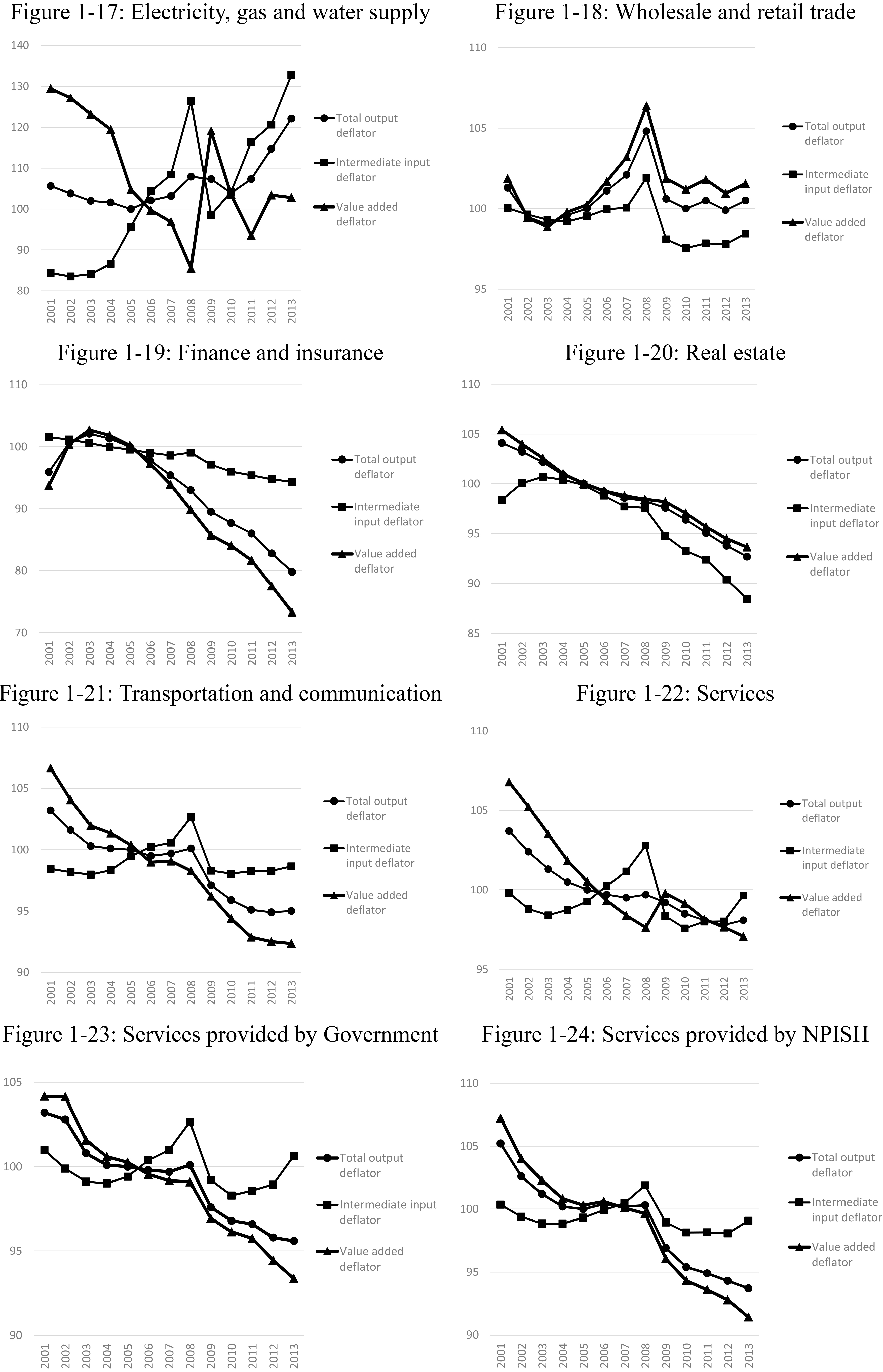
Figure 1.
The fluctuations in the deflators for total outputs, intermediate inputs and value added.
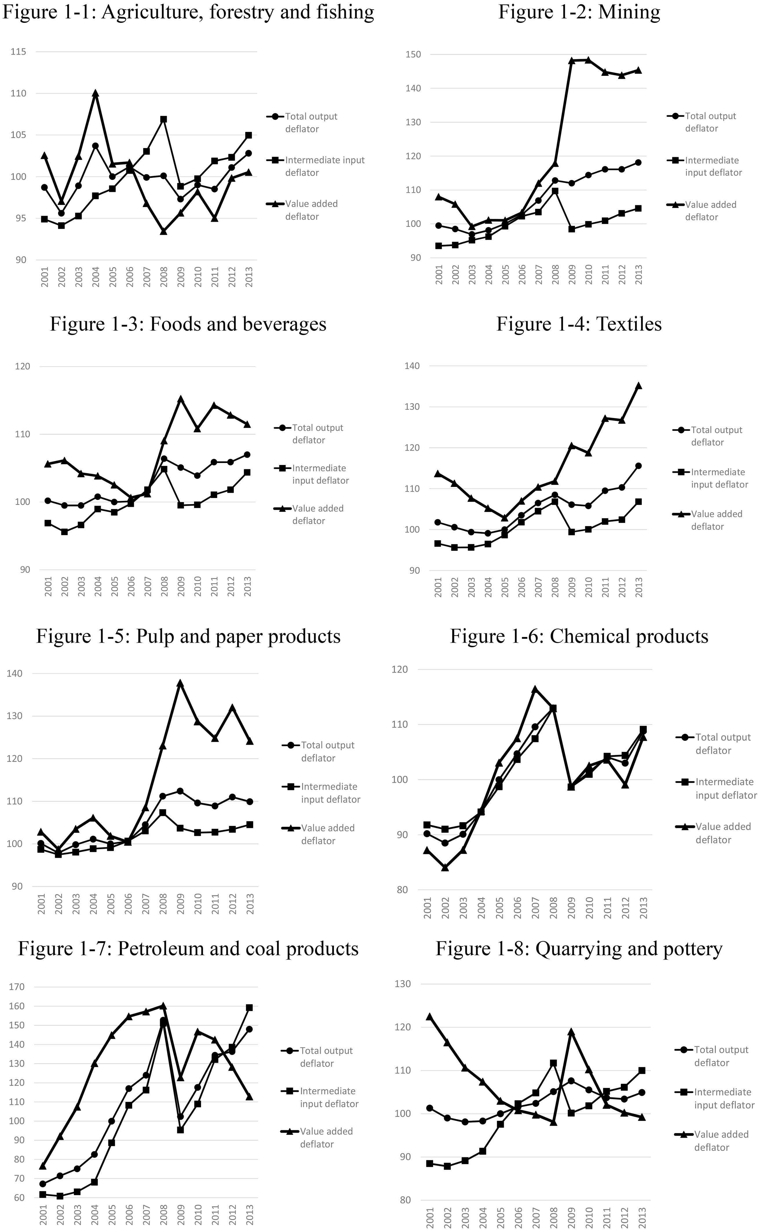
Figure 1.
continued.

Figure 1.
continued.
(less subsidiaries), and the operating surplus (and mixed income). Since wage deflators are unavailable in the SNA, we used the data published by the Research Institute for Advancement of Living Standards, which is the only Paasche wage index available in Japan. We made the deflator for taxes on production in the procedure described in the previous section. Since the original data of taxes on production included both taxes on products and other taxes on production, we divided it proportionally using the data published for the total economy. The observation period is from 2001 to 2013 calendar year.
Figures 1-1 through 1-24 depict the fluctuations in the deflators for total outputs, intermediate inputs, and value added for each industry. The correlation coefficients between the deflators are listed in Table 3. The main findings from the figures and the table can be summarized as follows:
(i) As shown in Eq. (2.2) above, output price is a weighted average of the input prices and the value added deflator:
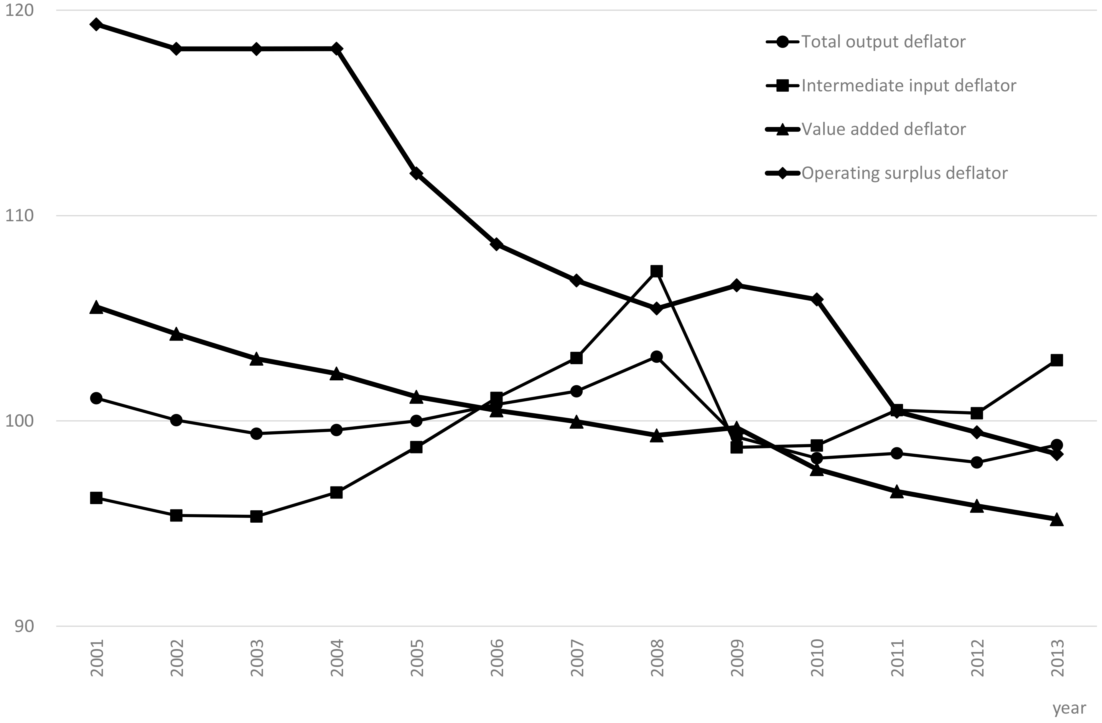
Figure 2.
The fluctuations in the deflators for value added, total outputs, intermediate inputs and operating surplus across all the industries.
(ii) The fluctuation patterns of the three deflators vary in one industry from another; there is no general trend. The observation tells us that industry specific value added deflators should be used to calculate real interest rates, which is supposed to be used for the investment decisions.
(iii) It is apparent that the deflators for the value added are more volatile than that for outputs and inputs because the former are the combination of the latter.
(iv) The value added deflators have higher correlation with output deflators rather than with input deflators. The correlation coefficients with output deflators are statistically significant at 5 percent level in 20 out of 24 industries and all of them are positive as expected. In contrast to this, the correlation coefficients with input deflators are statistically significant only in 9 industries, among which only two are negative as expected.
If you take look at the ‘electrical machinery and equipment’ (Figure 1-12), one of the dominant export industry of Japan, you will find a steep decline in the value added deflator during the first decade of the century because output price declined faster than the input prices. (See (i) above.) There is no wonder that the industry was reluctant to invest in new plants or equipment; gross capital formation of the sector at 2005 constant price declined by 31 percent between 2000 and 2013. This must be the reason why they lost their international competitiveness because new technologies are often embodied in the production facilities. It is a vicious circle because the lack of competitiveness depresses the value added deflator even further. In contrast to this, the value added deflator for ‘wholesale and retail trade’ (Fig. 1-18), a typical domestic industry, was more or less stable during the observation period. Gross capital formation of the industry at constant price rose 49 percent between 2000 and 2013, however, the value added of the industry at constant price increased merely 3 percent because of the sluggish economy.
Figure 3.
The fluctuations in the deflators for operating surplus, wage rate and the taxes across all the industries.
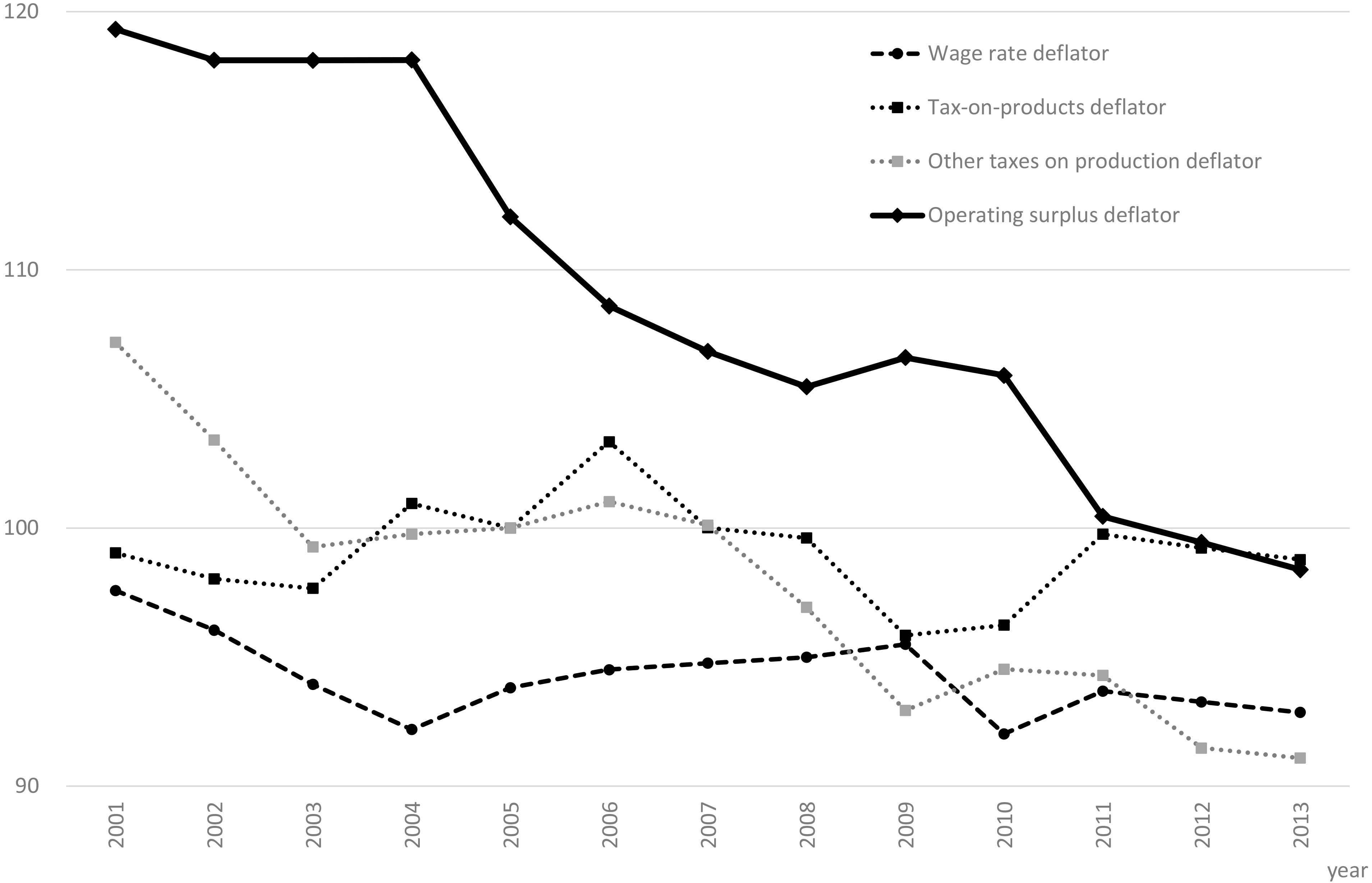
Figure 2 illustrates the fluctuations in the deflators for GDP, total outputs, intermediate inputs and operating surplus across all the industries. While output and input deflators peaked at 2008, the GDP deflator gradually declined throughout the observation period. It should be noted that, while the correlation coefficient between GDP and total output deflators is positive but not statistically significant, that between GDP and input deflators is not only negative as expected but also statistically significant at 5 percent level.88
The correlation coefficients between the operating surplus deflators and the value added and other related deflators are listed in Table 4. The main findings from the table are summarized as follows:
(v) Even though the levels are different, the value added and operating surplus deflators are highly correlated in most of the industries. The correlation coefficients are positive and statistically significant at 5 percent level in 17 out of 24 industries; the coefficients exceed 0.9 in nine industries.
(vi) The two tax deflators are positively correlated in 21 out of 24 industries; among which, the correlation coefficients are statistically significant at 5 percent level in 15 industries.
(vii) The operating surplus deflators tend to have relatively higher correlations with output and input deflators rather than with wage rates and the tax deflators.
Table 4
Correlation coefficients between operating surplus and related deflators (2000–2013)
| Correlation | Total output | Input and | Value added | Wage rate and | Taxes-on- | Other-taxes-on- | Taxes-on-products | |
|---|---|---|---|---|---|---|---|---|
| coefficients | and operating | operating | and operating | operating | products and | production and | and other-taxes-on- | |
| between | surplus | surplus | surplus | surplus | operating surplus | operating surplus | production | |
| deflators | deflators | deflators | deflators | deflators | deflators | deflators | ||
| 1 | Agriculture, forestry and fishing | 0.2258 | 0.7675 | 0.0978 | 0.9838 | |||
| 2 | Mining | 0.8721 | ||||||
| 3 | Foods and beverages | 0.8329 | 0.4219 | 0.9542 | 0.1322 | 0.4888 | ||
| 4 | Textiles | 0.3480 | 0.1561 | 0.8076 | ||||
| 5 | Pulp and paper products | 0.9345 | 0.7777 | 0.9542 | 0.5569 | 0.1552 | 0.6345 | |
| 6 | Chemical products | 0.9803 | 0.9538 | 0.9797 | 0.6813 | |||
| 7 | Petroleum and coal products | 0.1533 | 0.0022 | 0.4457 | ||||
| 8 | Quarrying and pottery | 0.9613 | 0.5862 | 0.0445 | 0.4432 | |||
| 9 | Primary metals | 0.5801 | 0.5396 | 0.7447 | 0.1412 | 0.4399 | ||
| 10 | Fabricated metal products | 0.4405 | 0.4292 | 0.3023 | 0.1694 | 0.5757 | ||
| 11 | General machinery | 0.5101 | 0.8063 | 0.4333 | 0.3470 | |||
| 12 | Electric machinery and equipment | 0.2824 | 0.2345 | 0.2373 | 0.1014 | 0.7112 | ||
| 13 | Transportation equipment | 0.5000 | 0.9653 | 0.7966 | ||||
| 14 | Precision equipment | 0.8454 | 0.6295 | 0.9394 | 0.3341 | |||
| 15 | Miscellaneous manufacturing | 0.0361 | 0.1571 | 0.1756 | 0.8602 | |||
| 16 | Construction | 0.3557 | 0.9283 | |||||
| 17 | Electricity, gas and water supply | 0.0581 | 0.9463 | 0.3124 | 0.5272 | |||
| 18 | Wholesale and retail trade | 0.4101 | 0.5904 | 0.5857 | 0.2214 | 0.6599 | ||
| 19 | Finance and insurance | 0.9879 | 0.8840 | 0.9909 | 0.0316 | 0.0439 | 0.9989 | |
| 20 | Real estate | 0.9855 | 0.8316 | 0.9960 | 0.7673 | 0.8615 | 0.7259 | 0.8795 |
| 21 | Transportation and communication | 0.9642 | 0.0681 | 0.9810 | 0.7982 | 0.7265 | 0.8882 | 0.9205 |
| 22 | Services | 0.8528 | 0.8529 | 0.5013 | 0.2289 | 0.8658 | ||
| 23 | Services provided by Government | 0.8967 | 0.0700 | 0.9277 | 0.6743 | 0.9071 | ||
| 24 | Services provided by NPISH | 0.8756 | 0.4750 | 0.8781 | 0.1610 | 0.8824 | ||
| Total | 0.3059 | 0.9665 | 0.4036 | 0.0222 | 0.8445 | 0.3228 |
Figure 3 illustrates the fluctuations in the deflators for operating surplus, wage rate and the tax deflators, taxes on products and other taxes on production, across all the industries. While other three indicators are somewhat fluctuating during the observation period, the operating surplus deflator declined significantly. There is a high correlation between the value added and operating surplus deflators; the correlation coefficient is as high as 0.966. There is a negative and significant correlation between the input and operating surplus deflators. Although the operating surplus deflator is significantly correlated neither with the wage rate nor taxes-on-products deflator, we do not know why, but we found a significant positive correlation with the other-taxes-on-production deflator.
4.2Decomposition of the value added deflators
Figure 4 depicts the decomposition of the value added deflator for each industry for 2013 in terms of Eq. (2.2) above. The line that lies above zero suggests that the output price effect surpasses the input price effect in any of the 24 industries listed there. Although, the import prices forms the larger part of the input price effect in ‘petroleum and coal products’ and ‘electricity, gas and water supply’ industries, the domestic prices account for more than half in most of the industries. The ratio of the output price effects to the input price effects is larger in the service industries comparing to the other industries. The ratio is smaller in the industries that heavily depend on imports.
Figure 4.
Decomposition of the value added deflator for each industry (2013).
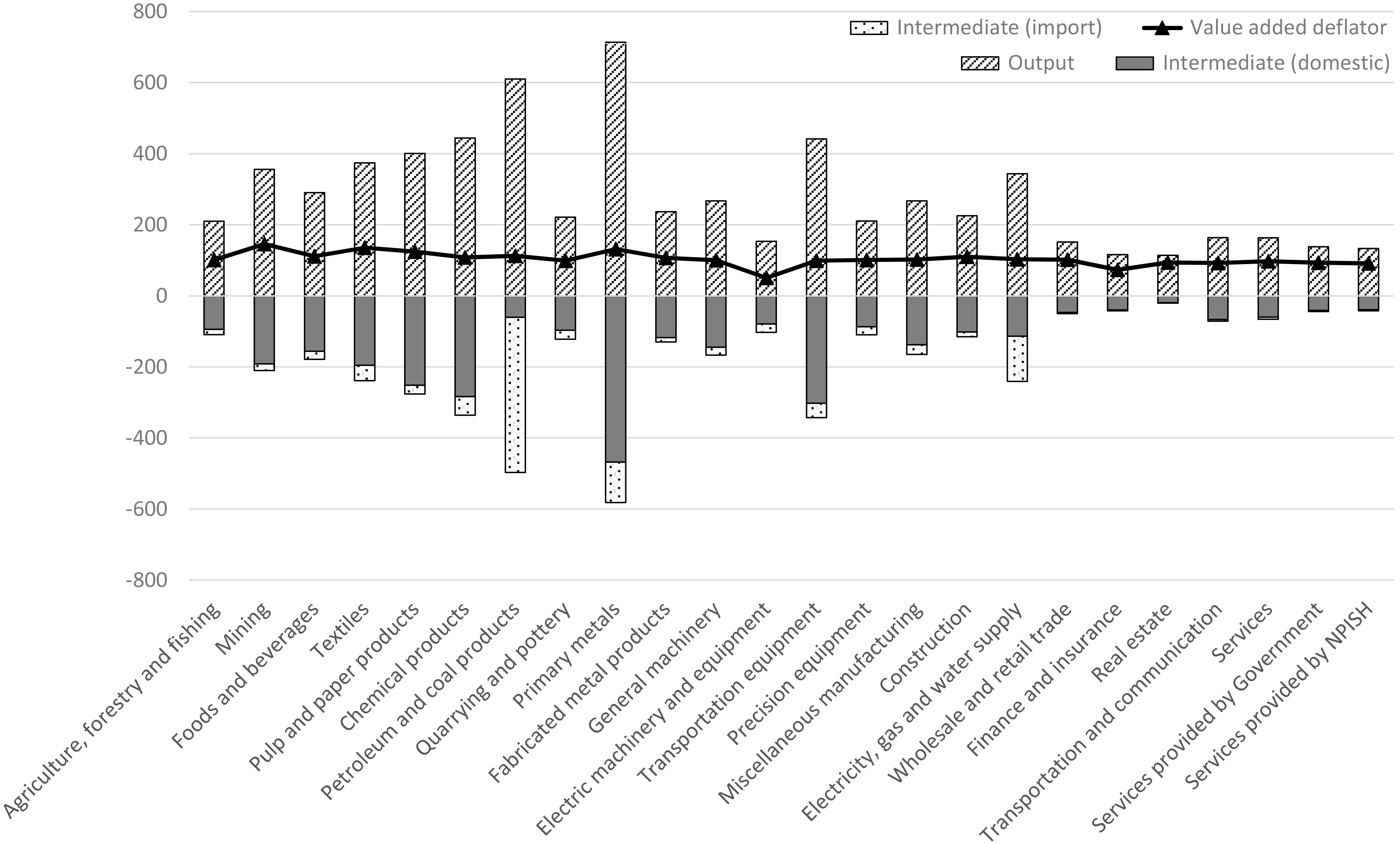
Figure 5.
Decomposition of the GDP deflator.
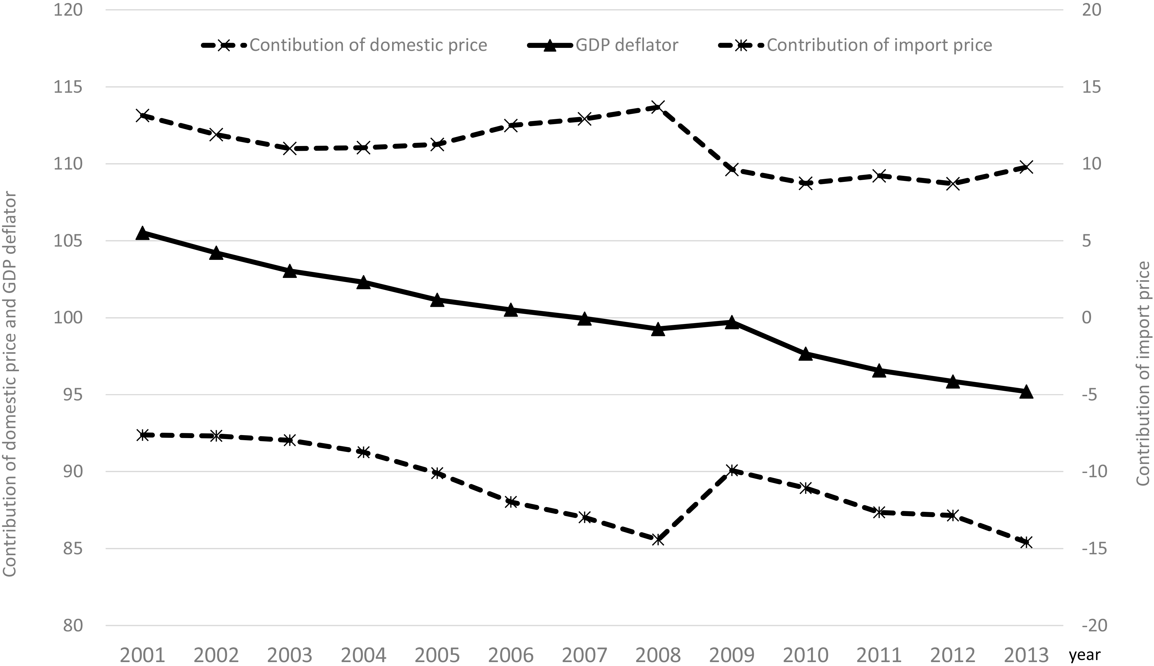
As shown in Fig. 5, the GDP deflator gradually declined during the observation period. The figure also depicts the decomposition of GDP deflator into domestic and import deflator effects. As Eq. (2.2) suggests, while domestic output deflator affects positively on the GDP deflator, import prices give negative effects on the deflator. Figure 5 clearly illustrates that the decline in Japanese GDP deflator during the observation period originated in the increase in the import prices. The decomposition of Eq. (2.2), which is illustrated in Fig. 6, tells us that only ‘transportation and communication’ significantly affected positively on the deflator. It should be noted however, this is not because the value added deflator of the industry rose, but because the production share of the industry increased considerably as the information technology and IT commerce rapidly advanced. In contrast to this, although the value added deflators for ‘mining’, ‘foods and beverages’ and ‘textiles’ increased as shown in Fig. 1, these industries affected negatively on the overall GDP deflator because of the decline in the production share. Summarizing Fig. 6, we can tell that the price drops in the domestic industries that supplies non-tradable goods and services were the direct cause of the decline in the GDP deflator. ‘Construction’ also negatively contributed to the GDP deflator despite its deflator hike because the real value-added share of the industry declined significantly during the observation period; ‘wholesale and retail trade’ also lost its share.
Figure 6.
Decomposition of the changes in the GDP deflator (2001–2013).
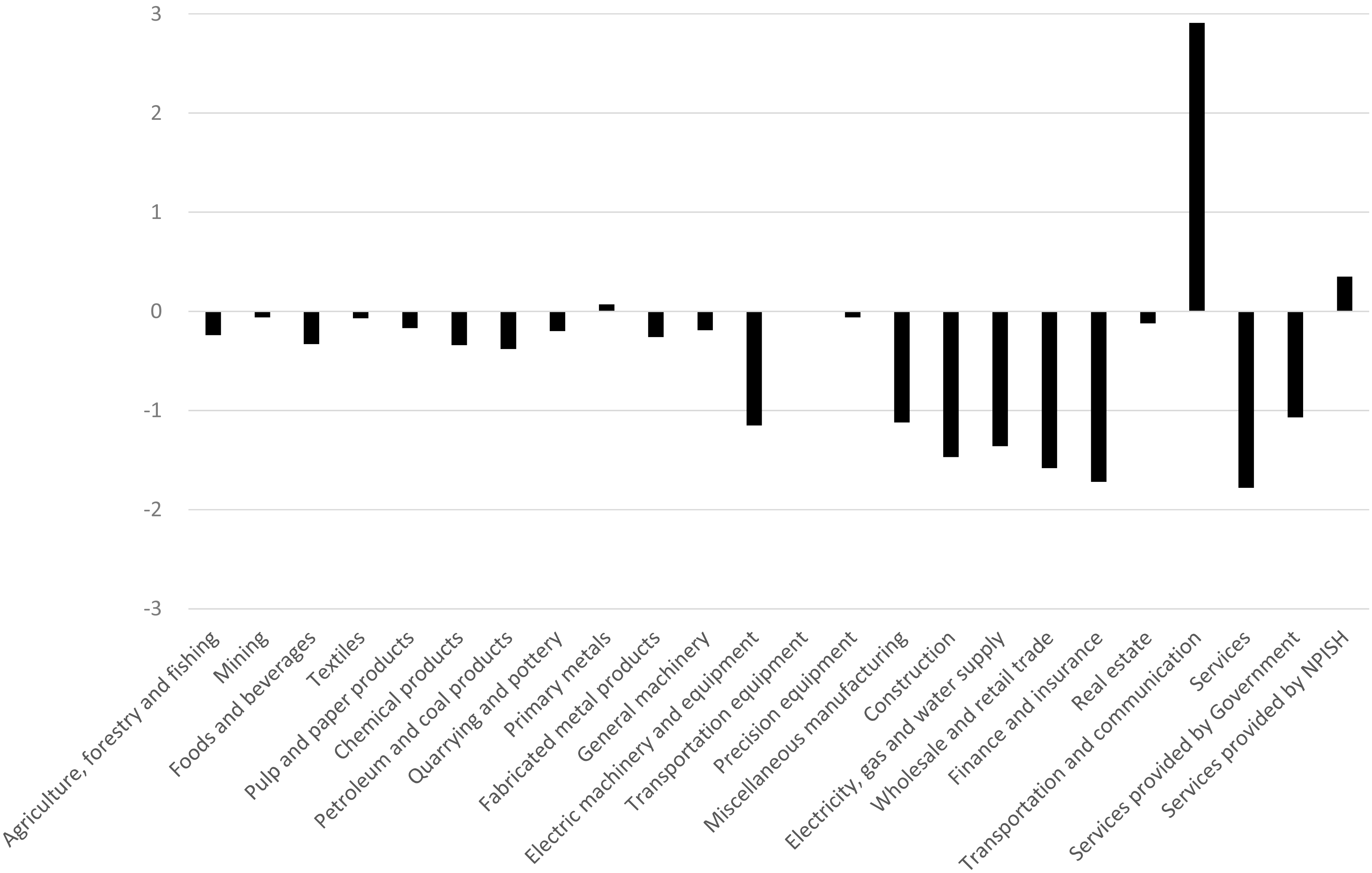
Figure 7.
Decomposition of the annual changes in the GDP deflator.
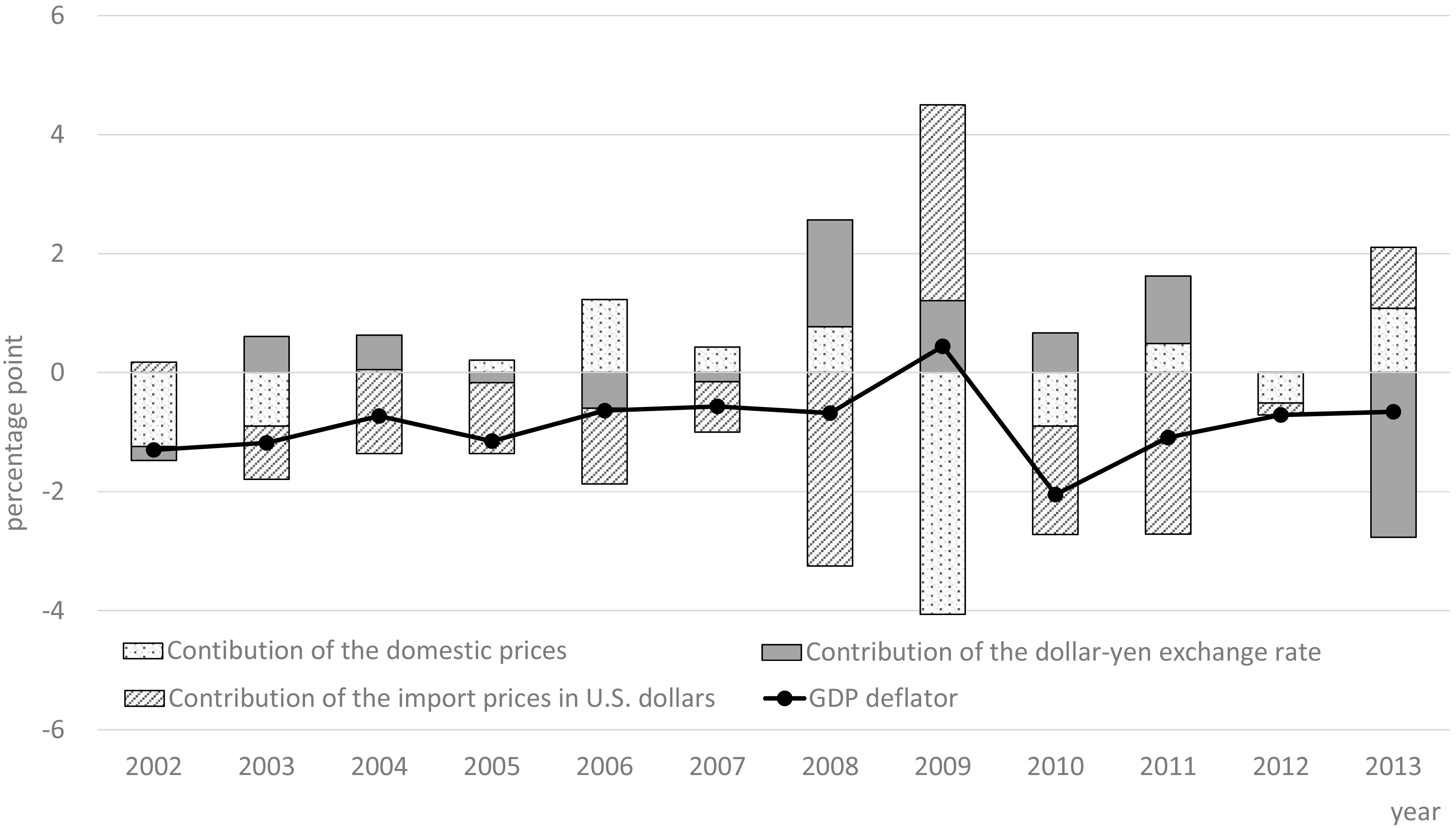
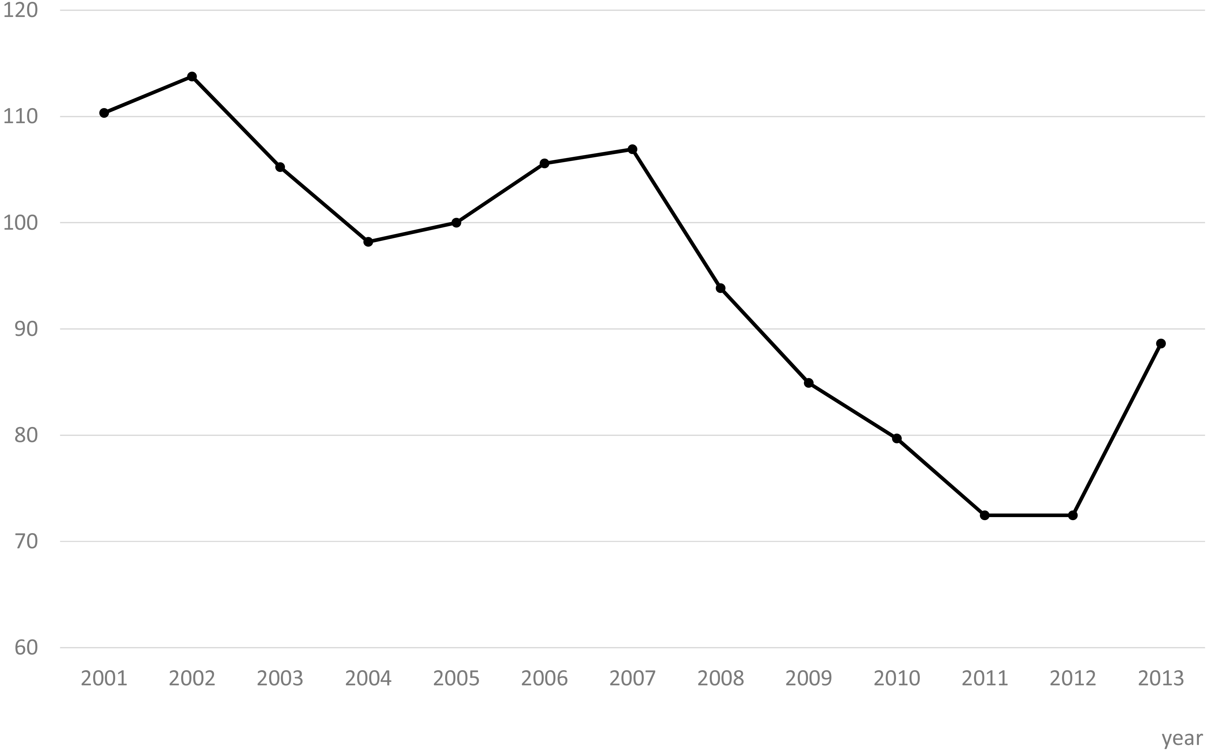
Figure 8.
The value of one U.S. dollar in Japanese yen (normalized to the 2005 exchange rate).
A great portion of the changes in the import prices is due to the fluctuations in the exchange rate because most of the Japanese imports are originally denominated in U.S. dollars. Thus, we decompose the import prices in Japanese yen as:
(32)
where
(33)
We can decompose the changes in the GDP deflator from year
(34)
The last two members of the last line of the above equation are the arithmetic mean of the Laspeyres and Paasche indices. While the second member of the line shows the effect of the changes in the dollar-yen exchange rate on Japanese GDP deflator, the last member indicates that of the dollar denominated prices. The results of the decomposition is depicted in Fig. 7. As displayed in Fig. 8, the value of Japanese yen peaked in 2004 and then declined toward 2007. After the U.S. subprime mortgage crisis, the yen was appreciated against U.S. dollar between 2008 and 2012 before plunging in 2013. Although the rise in the dollar-denominated import prices is the most conspicuous factor, the fluctuations in the exchange rate is also a dominant factor to determine the GDP deflator throughout the observation period. The yen’s appreciation after the U.S. subprime mortgage crisis in 2008 played an important role to keep the GDP deflator from declining, however, the depreciation of yen in 2013 had a significant effect to pull down the deflator only canceled by a hike in the dollar-denominated import prices and a surge in the domestic factors.
5.Concluding remarks
After the global financial crisis of 2008-2009, public debt in advanced economies has increased substantially. High levels of public debt in mature economies are a relatively new global concern after decades of attention on debt levels in developing and emerging countries. With slowly growing or declining workforces, as well as high capital-labor ratios, many advanced economies face a dearth of domestic investment opportunities, while the ageing society calls for more savings to prepare for the retirement. The governments are piling up deficits to close the saving-investment gap in the private sector. It is apparent however that the governments cannot accumulate deficits endlessly so that they must urgently promote the investments in the private industries. According to the Wicksell’s framework, it is obvious that lowering the market rate of interest is one of the best policies to boost the capital investment. But until recently there was a limit, what economists called the ‘zero lower bound’; it was long believed that when it comes to interest rates, zero is as low as you can go. More recently it has been breached; there is probably a limit to how much further we can go in that direction, but at the very least the latest developments show the zero lower bound is not as rigid as it was widely thought to be.
In 2009, Sweden’s Riksbank was the first central bank to utilize negative interest rates as a policy tool, with the European Central Bank (ECB), Danish National Bank, Swiss National Bank and, outside Europe, the Bank of Japan, all following suit. The lower and negative interest rates discourage the non-residents from buying the local currency so that it will be devaluated promoting exports and hindering imports; this can be another incentive to lower the interest rates. However, this paper reveals that the policy has some side effects. Figure 5, which is the GDP deflator decomposition based on Eq. (2.2), asserts that import price hike would inevitably depress the GDP deflator, the general indicator of the value added deflators. Equation (2.2) also confirms that the increase in import prices will adversely affect the value added deflators. It means that if lowering interest rate depreciates the local currency, it will depress value added deflators, and in turn, will discourage capital investments. In this sense, lowering interest rate is a double-edged sword; the governments and central banks should think twice before taking such a policy.
Notes
1 According to the definition of IMF [4], PPI includes not only output PPI but also input PPI and value-added PPI.
4 The decomposition procedure for taxes and subsidies on production is discussed in detail in paragraphs 9.1 through 9.11 of United Nations [11].
5 All the entries in the SNA-IO are VAT inclusive; the exceptions are exports and capital formation. We assumed zero-rating VAT for exports in our model as in Eq. (1) above, however, we did not make any adjustment for the capital formation in the present model because only a part of the VAT is deductible. VAT is generally known as ‘consumption tax’ in Japan.
6 Unlike in other countries, in Japan, the use table is made using the SNA-IO and the supply table using the procedure detailed in paragraph 3.83 of SNA 1968 manual, i.e.
7 OECD, Price Level Indices (indicator). doi: 10.1787/c0266784-en (Accessed on 25 June 2016). The OECD data gives the ratio of the domestic prices to the OECD average. Since both domestic and import price indices published by the BOJ is normalized to 2005, we used the OECD data for 2005 to normalize the import prices to 2005 domestic prices.
8 There is an apparent contradiction between the micro and macroscopic findings; this comes from the difference in the industrial composition between the nominal input and output.
9 The value of one U.S. dollar in Japanese yen normalized to the 2005 exchange rate.
Acknowledgments
The authors wish to thank Dr. Kirsten West, the editor in chief, and the anonymous referees for their constructive comments and useful suggestions. The authors are also grateful to Prof. Makoto Saito (Hitotsubashi University) and Prof. Kozo Miyagawa (Rissho University) for their discussions on the earlier version of the paper. This paper is funded in part by a Senshu University research grant.
References
[1] | Bernanke BS. Global Saving Glut and the U.S. Current Accounts Deficit. Remarks made at the Homer Jones Lecture, St. Louis, MO, (2005) April 14. |
[2] | Wicksell K.. Geldzins und Güterpreise: eine Studie über die den Tauschwert des Geldes bestimmenden Ursachen. Jena: Gustav Fischer; 1898 [translated by Richard Ferdinand Kahn. Interest and Prices: a Study of the Causes Regulating the Value of Money]. London: Macmillan; (1936) . |
[3] | International Labour Organization et al. Consumer Price Index Manual: Theory and Practice; (2004) . |
[4] | International Monetary Fund Statistics Department. Producer Price Index Manual: Theory and Practice; (2004) . |
[5] | Fabricant S. The Output of Manufacturing Industries, 1899–1937. New York: National Bureau of Economic Research; (1940) . |
[6] | Stone Richard. Quantity and Price Indexes in National Accounts, Paris: Organisation for European Economic Co-operation; (1956) . |
[7] | Moses LN. The Stability of Interregional Trading Patterns and Input-Output Analysis. American Economic Review. (1955) ; 45: (4): pp. 803-826. |
[8] | Chenery HB and Clark PG. Interindustry Economics. New York: John Wiley & Sons; (1959) . |
[9] | Diewert WE and Nakamura AO. Bias Due to Input Source Substitutions: Can It Be Measured? in Susan Houseman and Kenneth Ryder (eds.). Measurement Issues Arising from the Growth of Globalization. Washington D.C.: National Academy of Public Administration; (2010) . pp. 237-265. |
[10] | Reinsdorf Ml and Yuskavage Robert. Offshoring, Sourcing Substitution Bias and Measurement of U.S. Import Prices, GDP and Productivity. UTokyo Price Project Working Paper Series 41; (2014) . |
[11] | United Nations. Manual on National Accounts at Constant Prices. Series M, Number 64; (1979) . |
[12] | Watanabe G. The Features and Applications of the SNA Input-Output Account [in Japanese]. National Accounts Quarterly. 128; (2002) . |


