
Publishing public transport data on the Web with the Linked Connections framework
Abstract
Publishing transport data on the Web for consumption by others poses several challenges for data publishers. In addition to planned schedules, access to live schedule updates (e.g. delays or cancellations) and historical data is fundamental to enable reliable applications and to support machine learning use cases. However publishing such dynamic data further increases the computational burden for data publishers, resulting in often unavailable historical data and live schedule updates for most public transport networks. In this paper we apply and extend the current Linked Connections approach for static data to also support cost-efficient live and historical public transport data publishing on the Web. Our contributions include (i) a reference specification and system architecture to support cost-efficient publishing of dynamic public transport schedules and historical data; (ii) empirical evaluations on route planning query performance based on data fragmentation size, publishing costs and a comparison with a traditional route planning engine such as OpenTripPlanner; (iii) an analysis of potential correlations of query performance with particular public transport network characteristics such as size, average degree, density, clustering coefficient and average connection duration. Results confirm that fragmentation size influences route planning query performance and converges on an optimal fragment size per network. Size (stops), density and connection duration also show correlation with route planning query performance. Our approach proves to be more cost-efficient and in some cases outperforms OpenTripPlanner when supporting the earliest arrival time route planning use case. Moreover, the cost of publishing live and historical schedules remains in the same order of magnitude for server-side resources compared to publishing planned schedules only. Yet, further optimizations are needed for larger networks (>1000 stops) to be useful in practice. Additional dataset fragmentation strategies (e.g. geospatial) may be studied for designing more scalable and performant Web apis that adapt to particular use cases, not only limited to the public transport domain.
1.Introduction
Since it first broke onto the global stage more than 10 years ago, enabling unrestricted access to the raw data about a certain topic has been one of the guiding principles of open data.11 This way, data can be freely used by anyone to address particular challenges and provide novel services [18]. Public transportation (pt) stands among the most successful domains to embrace the principles set by the open data community [16], displaying important social and economic impact [34]. Millions of people22 around the world rely every day on open data-powered route planning applications (e.g., Google Maps, CityMapper, etc).
By definition, open data is free to be accessed and reused, but it is not free to publish open data [2]. Data publishers often impose access limitations over their public apis to cope with associated maintenance and scalability costs, which ultimately translates in lower data reuse and service innovation. For instance in the pt domain, a third party may be discouraged from developing new services supported on the public apis of a pt provider due to existing request limitations.
For the pt domain, open data have been traditionally shared through either data dumps or more complex Web apis, both with their own merits and disadvantages in terms of cost. On the one hand, raw data dumps constitute a low cost data publishing strategy for data publishers, but they impose high data management costs on reusers, who need to fetch, integrate and maintain up to date each dataset over which they want to offer a service. Additionally, data dumps become outdated at the moment of their creation, as they are not able to reflect any new changes on the data. On the other hand, more expressive Web apis (usually origin–destination http query interfaces) provide a low cost alternative for data reusers but might limit data accessibility by imposing request limitations due to high maintenance and scalability costs [1]. Moreover, they are often designed to serve specific purposes that cannot be adjusted by client applications. Data reusers are constrained to the query capabilities and the use case(s) supported by the api. For example, an api that calculates only the fastest routes in a pt network, may not be useful when trying to find routes that are wheelchair-friendly, or for different purposes than route planning.
These computational cost trade-offs between clients and servers (e.g, in terms of computational power, bandwidth, recency, etc) are captured by the Linked Data Fragments conceptual framework [56] and were considered for defining the Linked Connections (lc) specification [17]. lc puts forward one possible in between approach compared to data dumps and purpose-specific apis, designed to model and publish pt planned schedules. By organizing departure-arrival pairs (Connections) into chronologically ordered and semantically enriched data documents (fragments), client applications can autonomously traverse them to for example, evaluate route planning queries [15]. In this way data publishers need only to maintain a cacheable [17] and low-cost data interface, while reusers get full flexibility over up-to-date data without the cost of maintaining the dataset.
Next to planned schedules, access to live schedule updates (e.g. delays or cancellations) and historical data is fundamental for building reliable user-oriented applications and supporting other use cases based on pt data, such as smart city digital twin dashboards [36] or machine learning-based applications [33]. These are possible only if access to live and historical data is available. However, publishing these types of data further increases the computational burden of data publishers, resulting in often unavailable historical data and live schedule updates for most pt networks.
In this paper we apply and extend the Linked Connections approach to support cost-efficient live and historical public transport data publishing on the Web. We measure the impact in terms of server-side processing costs of publishing live and historical schedules compared to publishing just the planned schedules. We also study how api design aspects and pt network intrinsic characteristics may influence the performance of query evaluation for the most basic route planning problem, namely the Earliest Arrival Time (eat) problem. This is motivated by the fact that other, more complex types of route planning problems are normally addressed as extensions of eat. Therefore, optimizing performance of eat queries would consequently improve performance over related route planning scenarios. Additionally, we perform a comparison of the processing costs and performance (in terms of response time) of our lc-based approach vs the traditional and widely used route planning engine OpenTripPlanner.33
Concretely, our main contributions include: (i) a reference specification and system architecture that foresees efficient publishing of live schedule updates and allows to perform historical queries with access to precise granular data through http time-based content negotiation; (ii) empirical studies of publishing costs and route planning query performance over 22 different pt networks from around the world, considering different data fragmentation sizes and comparing to a traditional, non-semantic solution; and (iii) a cross-correlation of the performance results with each network’s particular size, average degree, density, clustering coefficient and average connection duration aiming on understanding how network characteristics may influence route planning query performance in practical implementations.
Results confirm that fragmentation size influences route planning query performance and converges on an optimal fragment size per network. Route planning query evaluation performance is shown to be highly correlated to network size (in terms of stops and connections) and to a lesser extent, to its density and average connection duration. Additionally, we show how knowledge of potential queries can drive a better design of data interfaces. Our approach also demonstrates superior scalability and in some cases better query performance (response time) for supporting efficient eat route planning query solving over smaller pt networks (<1000 stops). Yet, for larger networks further optimizations are needed to be useful in practice. Publishing live and historical schedules with our approach does not cause significant increase of server-side resources when compared to publishing planned schedules only. However response time of historical data fragments are significantly larger than current data fragments.
Insights on the factors that influence the performance of route planning query evaluation on lc-based applications provide a valuable asset for designing usable solutions that are fit for practical real world scenarios. For example, they can drive further geospatial fragmentation on top of pt networks, with the purpose of obtaining sub-networks that render higher performance for route calculations than performing the querying process over the networks as a whole. Clients could then interpret the semantically annotated hypermedia controls of such sub-networks to discover and download the right fragments of data to solve individual queries. This work stands as a contribution for the pt domain by demonstrating the feasibility of a cost-efficient approach for data sharing, and opening the door for new and innovative services and applications. It also shows how Semantic Web technologies can be applied not only to describe domain specific data, but also the interfaces that enable applications to consume it. The principles of meaningful data fragmentation and semantic annotation of interface hypermedia controls, applied on this work to a pt domain use case, could be reused on other domains and use cases. Thus building foundations for more generic, domain-independent and autonomous data applications.
The remainder of this paper is organized as follows. Section 2 presents an overview of related work around pt data modeling and sharing, route planning and live and historical data handling on the Web. Section 3 describes the proposed lc reference architecture. Section 4 describes the 22 different pt data sources considered for this work. Section 5 presents the details of the performed empirical studies on server-side cost-efficiency and route planning performance. Section 6 shows the obtained results. In Section 7 we discuss the results and the potential correlations of query performance with pt network intrinsic characteristics. Finally on Section 8 we present our conclusions and vision for future work.
2.Related work
The field of open data has been devoted to evolving the technologies that enable to share and reuse datasets, resulting in an ecosystem of data models, standards and tools. The Linked Data principles [8] are an example of this. Semantic Web and Linked Data technologies provide a common environment where data is given a well-defined meaning, allowing machines to interpret heterogeneous datasets by using common data models and reasoning [7,32].
Next to the Linked Data principles for aligning datasets, we also consider the computational cost of sharing data. Different trade-offs can be observed between publishing a data dump, or providing a querying api, as described by the Linked Data Fragments conceptual framework [55]. Regarding data models and apis for the pt domain, progress has been made as part of Mobility-as-a-Service (MaaS) ecosystems, aiming to provide integrated services for unified travel experiences in terms of transportation modes and payment [39].
In this section we present an overview of the main data sharing innovation efforts carried out in the pt domain, with route planning as its most prominent use case and an overview of such planning algorithms. Finally, we present related work regarding apis to publish live and historical data on the Web.
2.1.Public transport data models
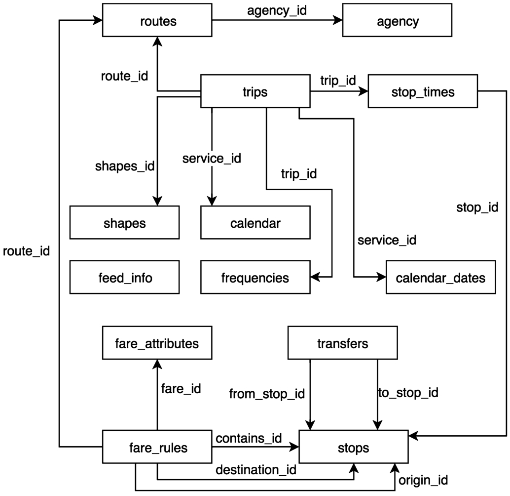
TriMet (Portland, Oregon) became the first pt operator to integrate its schedules into Google Maps in 2005. This collaboration fostered the creation of the General Transit Feed Specification44 (gtfs), which at the time of writing, is regarded as the de facto standard for sharing pt data. gtfs defines the headers of 17 types of CSV files and a set of rules that describe how they relate to each other (see Fig. 1). The most important files within gtfs can be listed as follows:
– stops.txt: Individual locations where vehicles pick up or drop off passengers.
– routes.txt: A route is a group of trips that are displayed to riders as a single service.
– trips.txt: An instantiation of a route. A trip is a sequence of two or more stops that occurs at specific time.
– calendar.txt: Dates for service IDs using a weekly schedule. Specify when service starts and ends, as well as days of the week where service is available.
– stop_times.txt: Times that a vehicle arrives at and departs from individual stops for each trip.
Fig. 1.
The gtfs data model and its primary relations.
The European Committee for Standardization created the Transmodel55 standard and its implementation NeTEx,66 to provide a description of conceptual models that facilitate exchanging pt network infrastructure topology and timetable data, among others. NeTEx was selected by the European Union, for the provision of an EU-wide multimodal travel information service, where every member state will publish their pt-related datasets through a National Access Point (nap). The official list of naps can be found online,77 however to this date only a few member states shared their data in NeTEx format, which could be attributed to the difficulty for pt operators to express their networks information in a new format and data model. Recent work by Scrocca et al. [46] relies on semantic web technologies to ease the transition of EU operators towards NeTEx.
Efforts to semantically describe the different concepts, properties and relations defined by the aforementioned data models, were made for the case of gtfs with the Linked GTFS vocabulary88 and for Transmodel with the Transmodel Ontology [11]. A comprehensive survey on semantic data models and vocabularies for the transport domain was performed by Katsumi et al. [37]. This survey does not focus only on pt but also includes other related aspects such parking and road traffic. The existence of so many different pt data models, sheds light on the lack of interoperability of the pt domain, but it also shows the efforts being made both from industry and public authorities to converge on well defined standards. Given it is mainly focused on modeling the concepts around pt planned schedules and that most pt data is available as such, we reuse Linked GTFS terminology in our approach to semantically describe pt important concepts such as stops, trips and routes. However, we take a different approach to model the granular behavior of individual trips. We pair together departure and arrival events into connections, in contrast to Linked GTFS that describes these events individually as a gtfs:StopTime. The reason for this is to facilitate the interpretation of these events to clients when evaluating route planning queries. Further details of our modeling approach are shown in Section 3.
2.2.Public transport Web interfaces
Public transport data are often found on the Web as data dumps or through apis. Static data dumps contain extensive planned schedules, which scale proportionally to the size and complexity of the transport network [27]. Most currently available dumps on the Web follow the gtfs model.99
Public transport apis on the other hand, can be found online spanning a wide spectrum in terms of openness, features and data structures. From the paid Google Directions1010 and CityMapper1111 apis, going over the freemium Navitia.io1212 api, to the completely free and open source routing engine OpenTripPlanner.1313 pt data interfaces in the wild are mostly available for route planning use cases, each with their own set of features and ad-hoc data structures. Some undergoing efforts from MaaS communities are trying to define standard api interfaces (e.g. MaaS Global1414 or TOMP1515 APIs) to harmonize data access when building MaaS applications. However, despite their heterogeneity in terms of data structures and semantics, a common pattern on their architecture design can be seen across all available apis: the servers of api providers are responsible for handling all the computational processing burden when evaluating queries, leading in practice to feature and access-restricted apis. We propose an alternative approach where servers only are responsible of publishing self-descriptive and departure time-sorted fragments of planned schedules, through a uniform interface and data model. This approach delegates the processing of queries to the client, in a more computational load-balanced architectural setup, that ultimately lowers the costs for data publishers and brings more flexibility over the data to client applications.
2.3.Formal representation of public transport networks
Beyond the standards and interfaces used to describe and share pt data, is also important to consider the different formal representations that have been proposed to analyze and understand pt networks. Traditionally, pt networks have been defined through formalisms from graph theory and complex network science [9], with different levels of abstraction that include among others, undirected graphs [30,54], weighted and directed graphs [13,50], time-expanded graphs [28], and time-varying graphs [29]. Across formalisms, vertexes normally represent physical stations in the network, and edges may represent different things depending on what is intended by the topology analysis [38]. When starting from timetable (i.e., planned schedule) data, edges are usually defined to represent connections among stops. In other words, an edge is present when there is at least one vehicle that stops consecutively in two stations, when following a predetermined route [22,47,48,57].
Different metrics have been proposed to analyze and obtain insights of pt networks. General graph theory-based metrics such as average degree [26], graph density [54], clustering coefficient [50], and also pt domain-specific metrics such as average connection duration [28] or directness of service [23] have been used to derive conclusions on the behavior of pt networks. For example, higher degree networks are typically associated with higher levels of network reliability [54], and higher clustering coefficients reflect higher accessibility among stations [40]. Hong et al. [35] present a compilation of studies that apply complex network metrics over different pt networks. However, even though graph metrics have been correlated to process performance in different application domains, for example to assess data quality change on dynamic knowledge graphs [31], to the best of our knowledge there are no studies that investigate potential relations of network graph characteristics and route planning query performance. We perform an evaluation in this direction and analyze how specific pt network graphs characteristics may influence route planning performance.
2.4.Route planning algorithms
From a traveler’s perspective, route planning is the most popular use case over pt data and thus has been extensively studied throughout the years. Bast et al. [3] and Pajor [42] present a comparative analysis of multiple route planning algorithms over pt networks, road networks and combination thereof. Most pt algorithms are defined as extensions of Dijkstra’s algorithm [25] using graph-based formalizations such as time-dependent [10] and time-expanded [43] graphs to model networks. Other alternative approaches such as raptor [19], csa [24], Transfer Patterns [4] and Trip-based routing [58] exploit the basic elements of pt networks to calculate routes directly on the planned schedules.
A pt route planning query can be further specified into more concrete problems depending on the concrete use case. The literature defines different types of route planning query problems, usually defined in terms of Pareto-optimizations, that require specific algorithm implementations with varying levels of complexity [20,24]. The simplest and most common one is the Earliest Arrival Time problem, where given an origin, destination and a departure time τ, an algorithm should render a journey departing no earlier than τ and arriving as soon as possible. Other common problems include the Profile problem variants, to calculate the set of possible journeys within a time range or the Multi-Criteria problem for considering additional optimization criteria over the resulting Pareto set (e.g., maximum number of transfers or transport modes).
Each algorithm requires specific data structures and indexes in order to find possible routes over pt schedules. The time-based sorted structure of our publishing approach fits the requirements for executing route planning algorithms based on the Connection Scan Algorithm (csa). In our evaluation, we take an implementation of csa to a client-side application and use it to evaluate Earliest Arrival Time queries.
2.5.Live and historical data on the Web
Live data is critical for supporting practical use cases that are useful in real scenarios. It is particularly important for pt route planning given that in practice, schedules change due to unforeseen delays and cancellations, which could render calculated routes unfeasible. gtfs-realtime1616 and siri,1717 are among the main reference standards for live schedule updates and vehicle positions. Both define protocols to exchange live updates for planned schedules, modeled using gtfs and Transmodel standards respectively. Most currently available pt live data on the Web use the gtfs-realtime standard [1].
In the same way, historical data is fundamental for some use cases in the pt domain. Machine learning-based algorithms require training data that closely reflect reality to make predictions on a certain scenario [33]. pt operators require to perform statistical analyses based on accurate data of past events to asses the performance of their networks [5]. Such data may already exist within operators information systems, but unfortunately is not commonly made public for third party reuse. The unavailability of public historical data may be motivated by operators strategic business choices or simply by the inherent costs of maintaining a dedicated public API for this purpose. Either way limiting the development of novel use cases. An example of public historical information can be found by accessing the Belgian trains delays and disruptions site1818 through the wayback machine service of the Internet Archive initiative. However besides not being machine readable data, this does not constitute a reliable source as snapshots are not consistently archived.
In an effort to standardize the way historical information is accessed on the Web the ietf published the RFC 7089,1919 also known as the Memento framework [51]. Memento defines a protocol over http to perform time-based content negotiation of Web resources among clients and servers. The latest version of a resource is defined as the original resource uri-r. Previous versions of uri-r are defined as Mementos uri-mi with
The idea of accessing and querying historical versions of data through time-based content negotiation, has been already explored by Taelman et al. for the case of time-annotated knowledge graphs [53]. In our approach we apply this principle to provide access to the history of changes of pt network schedules, which are also represented as knowledge graphs in the form of rdf. In this way we bring together both (versions of) planned and live update data, which can be queried in a cost efficient way. Design and implementation details are presented in the next section.
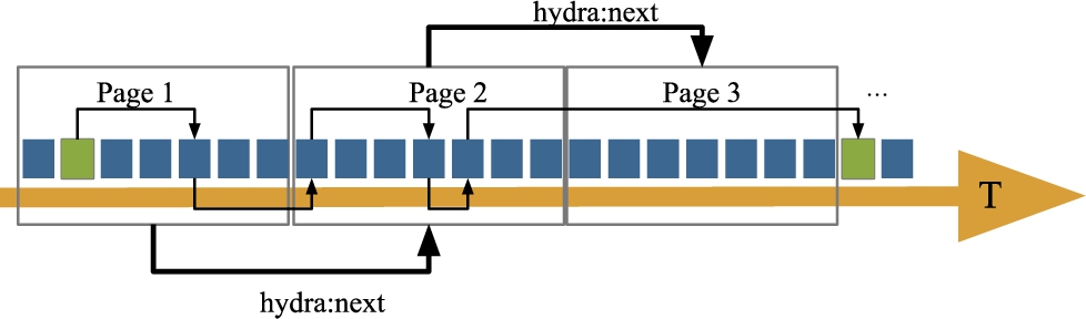
Fig. 2.
Depiction of chronologically ordered linked data documents containing lc (represented by the blue blocks). Each document contains links (hydra:next labeled links) to the previous and next document in the collection, that can be traversed by clients to found routes across the pt network. The green blocks represent the departure and arrival connections of an hypothetical route planning query and the thinner links comprise the route solution that will be computed by scanning the collection.
3.The Linked Connections framework
In previous work we introduced Linked Connections (lc)2020 as a light-weight linked open data interface for publishing pt planned schedules. It allows applications to evaluate route planning queries on the client [15,17]. lc models pt planned schedules through departure-arrival pairs called Connections, which are ordered by departure time, fragmented into semantically enriched data documents and published on the Web over http (see Fig. 2). Despite being designed mainly to optimize the implementation of route planning use cases, other use cases requiring different types of querying, could still be supported by the lc approach, even though other alternatives may be more efficient for specific cases. A lc interface publishes the unmodified raw data of transport schedules which for example, could allow an operator interested in finding the busiest stations during peak hours in the last month, to implement an application that traverses the lc collection to find an answer to this query, without having to implement dedicated interfaces on the server-side.
Our previous work on lc mainly focused on demonstrating the feasibility of this approach and its benefits in terms of cost-efficiency for publishing pt planned schedules on the Web. We showed that lc achieves a better cost-efficiency by consuming considerably less computational resources on the server-side, when compared to traditional route planning origin-destination query interfaces. The price of this decreased server load is paid by an increased implementation complexity of client-side applications and a higher bandwidth requirement, which is three orders of magnitude bigger. This increased cost for application developers could be mitigated by setting the lc consumer as part of their server infrastructure, which in turn could expose traditional origin-destination apis [17]. In our previous work however, we did not study how live pt data could be managed and accessed efficiently, nor how historical data could be archived and queried. We started exploring an approach to handle live and historical data and proved its feasibility through a preliminary demonstrator [45]. Yet, a general overview of a lc-based system and a more detailed description of how its individual components could be implemented were still missing. To summarize, in previous work we:
In this paper we build on these previous works and provide the following contributions:
– A generalized architecture to publish planned, live and historical pt schedules.
– An study of the factors that influence route planning query performance over a lc interface.
– A comparative study of the cost-efficiency and performance of our approach, against the traditional non-semantic solution OpenTripPlanner and an assesment of the added costs of publishing live and historical schedules.
Next, in this section we (i) describe the semantic specification of lc data, showing the requirements that shape the lc model; (ii) define a reference modular architecture for implementing lc-based solutions and (iii) describe in detail how we manage and provide efficient access to live and historical pt data.
3.1.Linked Connections specification
We created a specification that describes the different requirements to implement a lc data publishing interface and a set of considerations for client applications implementing route planning solutions.
lc uses Connections as the fundamental building block of pt data. A connection describes a departure-arrival event between given two stops, that occurs at a certain point in time and without intermediary halts. In other words, a connection must contain the definition of at least a departure stop, an arrival stop, departure time and an arrival time. Additionally, a connection is related to a specific trip. This is important for client applications to interpret sets of connections as part of independent trips during route plan calculations.
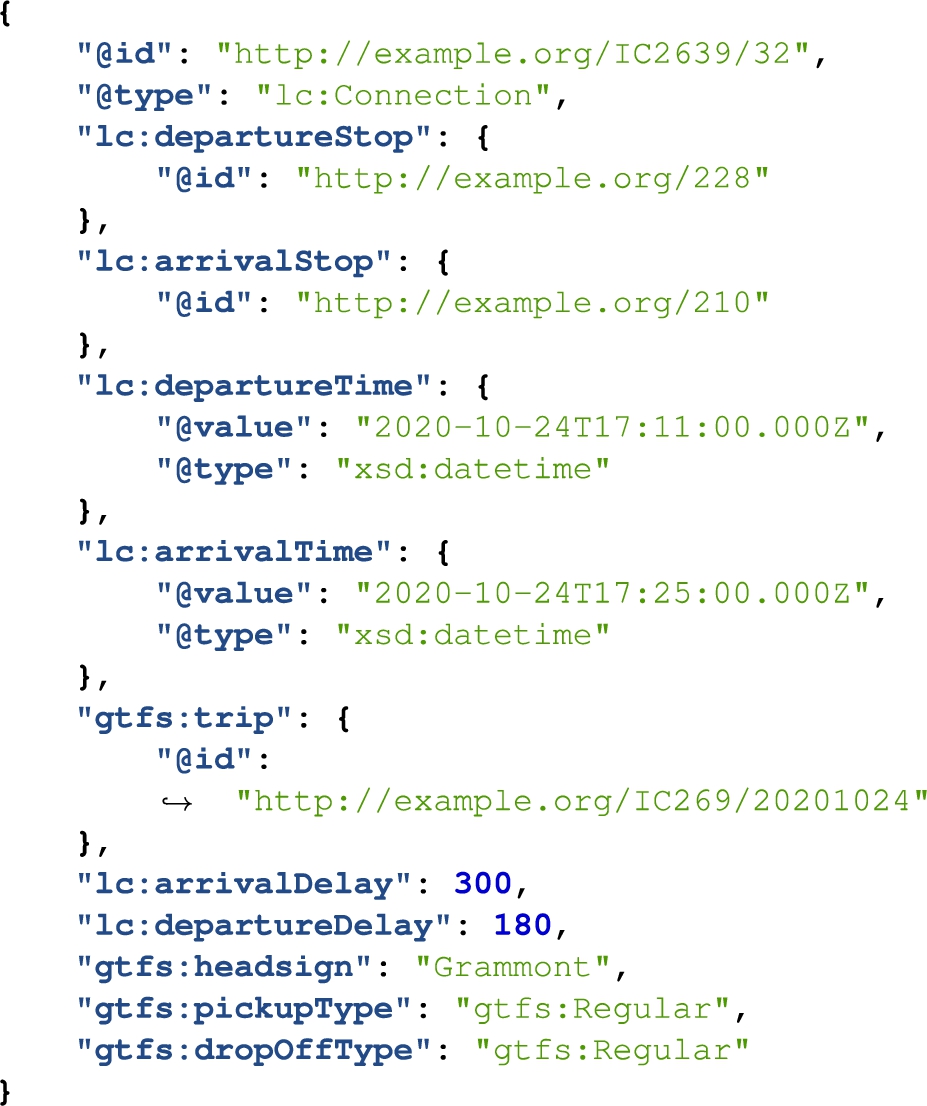
We define connections as rdf graphs, following the Linked Data principles. lc data interfaces should therefore publish data, in at least one of the rdf compliant serializations (e.g., turtle, JSON-LD, N-Triples, etc). Connections are described by means of the linked connections ontology and also with terms from the Linked GTFS vocabulary. The main concepts to semantically model and represent connections are the lc:Connection rdf class, together with the predicates that reference departing and arrival stops and times. Table 1 describes these terms and Listing 1 shows an example of a lc using the JSON-LD serialization.
Table 1
Main terms used to model and semantically define lc. The prefixes lc and gtfs stand for http://semweb.mmlab.be/ns/linkedconnections# and http://vocab.gtfs.org/gtfs.ttl# respectively
| Term | Description |
| lc:Connection | Describes a departure at a certain stop and an arrival at a different stop. |
| lc:CancelledConnection | Represents a previously scheduled departure and arrival that won’t take place anymore. |
| lc:arrivalTime | The time of arrival at a certain stop. When a delay is announced, it will show that actual time of arrival. |
| lc:arrivalStop | A vehicle will stop here on arrival. |
| lc:departureTime | The time of departure at a certain stop. When a delay is announced, it will show that actual time of departure. |
| lc:departureStop | A vehicle will depart here. |
| lc:arrivalDelay | The time (in seconds) in which the lc:arrivalTime differs from the scheduled arrival time. |
| lc:departureDelay | The time (in seconds) in which the lc:departureTime differs from the scheduled departure time. |
| gtfs:trip | Indicates the specific trip to which a connection belongs to. |
| gtfs:pickupType | Indicates if passengers may board the vehicle at the departure stop. |
| gtfs:dropOffType | Indicates if passengers may get off the vehicle at the arrival stop. |
| gtfs:headsign | Contains the text that appears on a sign that identifies the trip’s destination to passengers. |
Listing 1.
LC formatted in JSON-LD. The properties departureDelay and arrivalDelay indicate that live data is available for this Connection
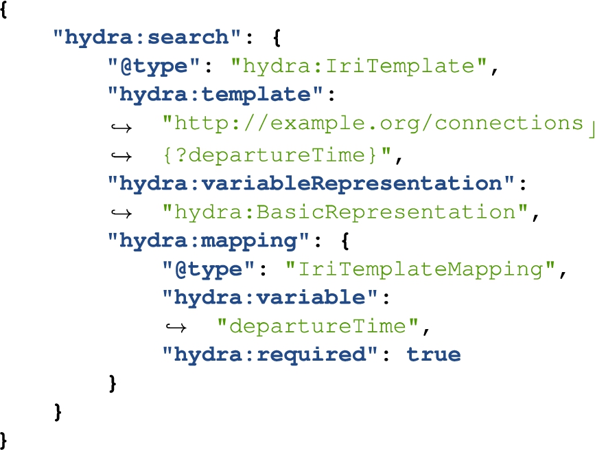
Listing 2.
Hydra search form defining a uri template for accessing lc documents with connections departing no earlier than the requested time. It explicitly defines how clients can request specific documents and the variables they are allowed to use. In this case the only variable is the departureTime
A lc data interface publishes pt network schedules as a chronologically ordered paged collection of connections over http. This particular design is motivated to support the execution of csa-based algorithm implementations on the client side. The reason for choosing csa as the main supported route planning algorithm is related to the relative simplicity of publishing csa’s required data structure, namely a chronologically ordered collection of lc:Connections, compared to more complex structures and set of indexes required by other state of the art route planning algorithms. The semantic definitions provided by Linked Connections could still be reused to publish the same data, organized in different structures, to enable clients performing other algorithms. For example, by exposing the ordered set of lc:Connection’s per gtfs:Trip, a client could independently implement the raptor algorithm.
Each lc document should be served with the appropriate headers to enable both server and client-side caching. High cacheability of data is one of the biggest advantages of the lc approach, in terms of cost-efficiency and scalability for data publishing interfaces. Document responses require also to enable cors (Cross-Origin Resource Sharing), given that data will be accessed by clients from multiple origins. Furthermore, lc defines semantically annotated hypermedia controls as part of every document’s metadata. The purpose is to allow clients to discover and automatically navigate the pt schedules. The hypermedia controls are defined using the Hydra vocabulary,2121 including the following terms:
– hydra:next: Indicates the uri of the next lc document in the collection.
– hydra:previous: Indicates the uri previous lc document in the collection.
– hydra:search: Defines a uri template indicating how clients can query for a document in the collection, containing connections starting from a specific time (see Listing 2).
Fig. 3.
Reference architecture for lc-based systems.
3.2.Linked Connections reference architecture
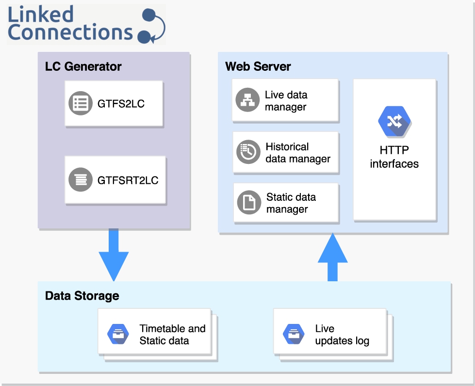
A lc system’s main purpose is to publish pt schedules as a chronologically ordered collection of vehicle departures over http, while taking into account live updates to the original schedules and keeping historical data available for later querying. To this end we define a reference architecture (see Fig. 3) with three main modules that generate, store and serve lc. We also provide a complete and open-source reference implementation of this architecture as a Node.js application.2222
LC Generator This module is responsible for creating lc. It takes gtfs (planned schedules) and gtfs-realtime (live updates) data sources as input, given that most pt data is available in these formats. We provide implementations for both modules through the gtfs2lc2323 and gtfsrt2lc2424 Node.js libraries. However, thanks to the modular nature of the architecture, it is possible to replace these modules with any other interfaces capable of creating lc from different data sources (e.g., Transmodel, apis, etc). One of the most important aspects that need to be considered when creating lc is the provision of a stable identification (uri) strategy that remains valid across versions of the data sources. We make possible to define such strategy using uri templates as defined by the RFC 6570 specification.2525
Data Storage The output of LC Generator is received by this module, which proceeds to fragment and store the data according to a given fragment size. Static lc (i.e. data coming from a planned schedules) are stored as individual files that correspond to the documents of the time-ordered lc collection. Additionally, files containing the set of stops and routes of the pt network are kept to be served as static documents too, since they are usually needed by route planning applications. Live updates are also stored as files following a log-like approach, where delays, ahead of time and cancellation reports for every single connection are written down. Files in both cases are named using the first departure datetime they contain to facilitate later connection lookups.
Web Server This module defines the interfaces through which lc and other related pt data may be accessed by client applications. The http interfaces supported by the lc Web server are as follows:
– /connections: This interface provides access to the lc documents. It receives a departure time query parameter, as seen in Listing 2, used to obtain the document with connections departing on a specific time. If not provided it will resolve to the current time document.
– /stops: This interface returns the complete set of stops defined for the pt network as a static document. Stops are described with terms from the Linked GTFS vocabulary.
– /routes: This interface returns the complete set of routes available in the pt network as a static document. It includes information like route number/name, color or type of vehicle (e.g. metro, tram, bus, etc) which are also described with the Linked GTFS vocabulary. Route data are useful for displaying route plan results in user applications.
– /catalog: This interface provides a catalog definition given using the dcat vocabulary. It describes the different data sources published on the server, including their access URLs, supported media type formats, last issued date, license information, among other metadata. Its main purpose is to increase discoverability of the data.
The Web Server module also contains submodules responsible for resolving lc documents requests in an efficient way. Particularly the architecture defines three specific submodules for supporting requests that include live data, historical data and also static data. The live data manager submodule takes care of serving lc documents that include the latest connection updates. A detailed reference implementation of this submodule is presented later in Section 3.3. In the same way, the historical data manager handles serving previous versions of lc documents through http time-based content negotiation using the Memento protocol. A reference implementation is detailed in Section 3.4. Lastly, the static data manager handles requests for static resources, namely stops, routes and the server’s dcat metadata.
3.3.Serving live Linked Connections
Managing and serving live schedules updates, without sacrificing the cost-efficiency of the data publishing interface, constitutes one of our main contributions in this paper. In previous work we studied pushing (server-sent events) and polling (http) interfaces to exchange live pt data with client applications and keep route planning results updated in a cost-efficient way. We found that a polling approach consumes less resources on the data publishing side and clients only experience a slightly higher bandwidth consumption, compared to a pushing approach [44]. However, our implementation for serving live lc was done in a naive way. We merged scheduled lc documents with their latest updates on request time, with significant negative impact on response times.
We introduce a more elaborated approach to reduce response times of lc document requests without compromising cost-efficiency. The set of departure time-sorted Linked Connections
Fig. 4.
Depiction of the lc AVL tree reacting to a schedule update. In this example,
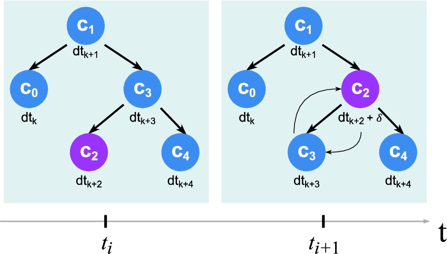
The AVL tree is initially generated by scanning over the scheduled lc, kept by the Data Storage module on server boot time. Once created, the live update logs are constantly monitored and trigger tree reorganizations when new reports are received.
3.4.Serving historical Linked Connections
Another important contribution of this paper, is providing the ability for serving historical lc data. We allow querying not only for past planned schedules but also for historical live data reports. This means it is possible to obtain the actual vehicle departures as they were reported at different points in time. For example, we could request for the departures of yesterday at 08:00 h as they were expected to be yesterday at 07:00 h and also later at 07:50 h, seeing possibly that a connection that was on time at 07:00 h was later reported to be delayed at 07:50 h. In this way is possible to reproduce the stream of events of a pt network at a granularity given by the frequency of live update reports. Access to this data could support analytical studies to better understand the behavior of pt networks and also other use cases that rely on historical information of trips to provide recommendations to travelers [12].
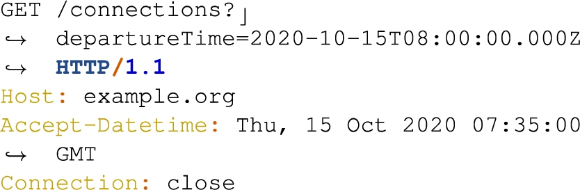
We make this possible through the http Memento protocol. Given the document-based nature of lc, it is possible to request past versions of a specific document, as it was at a certain point in time. Memento defines different patterns to perform time-based content negotiation. We implemented pattern 1.1 where uri-r = uri-g and 302-style negotiation is performed. This means that the original resource acts as its own time gate and clients receive a 302 http response containing a Location header with the uri of the Memento. An example get request is shown in Listing 3, asking for connections departing from 08:00 h as they were reported at 07:35 h. The specific version time is given through the Accept-Datetime header, as defined by the Memento protocol.
Performing these kind of queries is possible thanks to the way lc are stored in the Data Storage module, as separate sets for both scheduled and live update data. When a Memento request is received, the system gets first the lc fragment containing the originally scheduled connections. This first step may seem trivial but is necessary to consider that there may be multiple versions of overlapping planned schedules. Therefore, the system needs to select the version issued closest to the specified Accept-Datetime date, before integrating live reports. Then the system goes over the live update logs for this specific lc document, retrieving and merging all the updates received up until the Accept-Datetime date. As mentioned in Section 3.3 this could be considered as a naive approach which may increase response times of individual lc fragments. However we part from the assumption that historical data queries are not as performance-critical as live data queries for route planning purposes, and can still be resolved within reasonable time following this approach.
Listing 3.
Hydra uri template for accessing lc documents containing connections with departure times equal or bigger than the requested time
3.5.Linked Connections client
The chronological ordered collection of connections defined by a lc system, is a fitting data structure to perform the Connection Scan Algorithm (csa), proposed by Dibbelt et al. [24]. Given a departure stop, arrival stop and departure time, csa will go over the collection of connections, progressively building a minimum spanning tree of reachable destinations. The algorithm performs this process until it reaches the desired arrival stop, rendering in this way, the earliest arrival journey possible (if any). This provides a solution for the Earliest Arrival Time problem. In the case of lc, a client performing the csa algorithm can scan through the collection of connections by downloading lc documents and following the defined hypermedia controls to traverse it. We provide an implementation of csa on the Planner.js JavaScript library,2626 which can be used both on server (Node.js) and client-side applications.
4.Datasets and metrics
For testing our proposed approach we conducted a set of evaluations (see details in Section 5) considering data from 22 real-world pt networks. Aiming on getting generalizable results, we selected a representative set of heterogeneous pt networks in terms of modes of transport and geographical coverage (urban, regional, national and international). In this section we describe these pt networks, our modeling approach to represent them and a set of measured graph topological characteristics.
We rely on the definitions of network topology introduced by Kurant and Thiran [38]. In particular, we use graph topologies in space-of-stops, to reflect the traffic flow of the pt transport networks. Considering that these type topologies are inherently time-dependent, we opted to model them as Time-Varying Graphs (
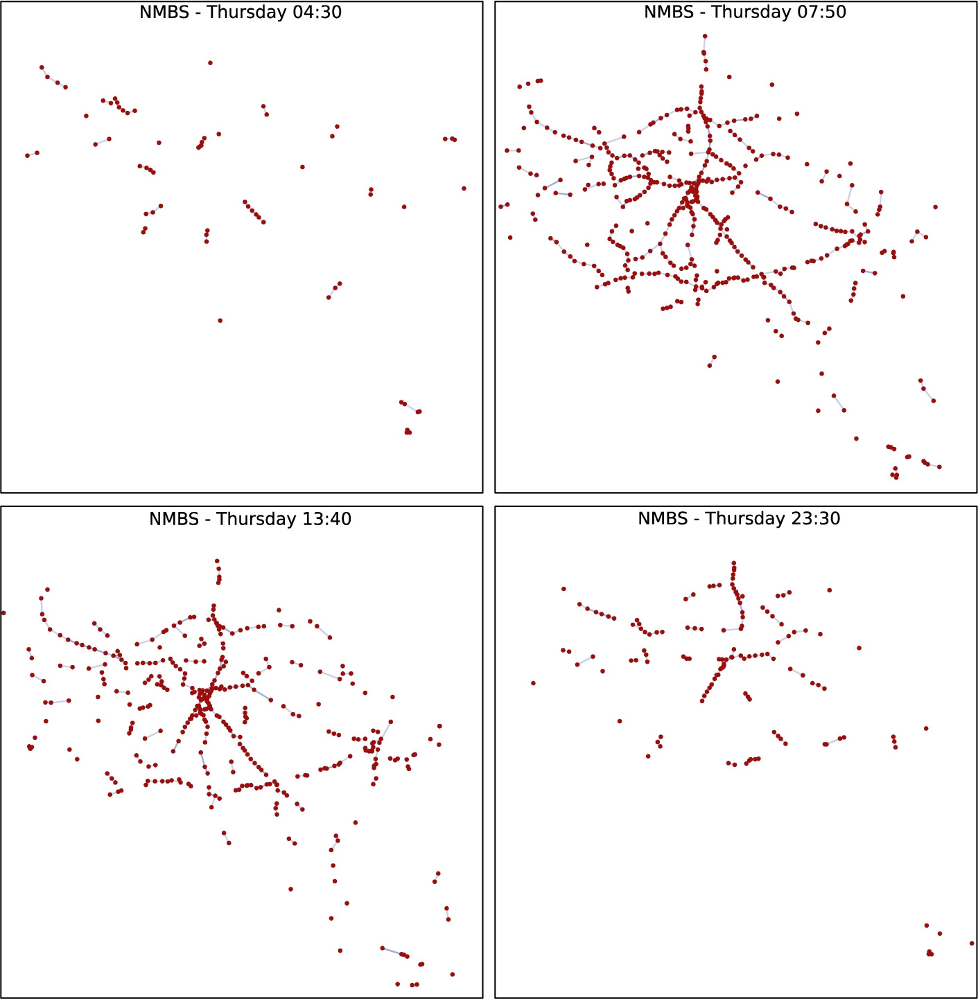
Fig. 5.
Network graph snapshots of the Belgian train pt operator NMBS, taken over the busiest day of their timetable. It can be observed how the topological structure of the network varies throughout the day, in particular showing a higher amount of connections between stops during peak hours.
TVGs are typically defined by an ordered-set of T snapshot graphs
Based on related work about analytical frameworks to study pt networks [13,29,30,50,54], but mainly aiming to reflect their dynamic behavior and topological changes over time, we decided to observe the following graph properties of each network:
– Size: Size is a basic graph property, in this case interpreted as the total number of stops
– Average Degree: Degree k is measured on a vertex as the sum of its incoming and outgoing edges, interpreted in this case as departing and arriving connections. For every graph snapshot
The average degree of a network shows how connected is each vertex in the network [35].– Density: Graph Density D is an indicator aimed at measuring how close is the network structure to a complete graph. It is defined as the ratio of existing edges and the total number of possible edges in the network. We calculated the total Density of the
An increased density is usually an indication of reduced time travelling in pt networks [54].– Clustering Coefficient: Clustering Coefficient C is a measurement of how well connected are the neighbors of a given vertex. Is defined as the ratio of existing edges and total possible edges among neighbors of a vertex, which is averaged for all the vertexes in the network. We measured the total C of the
where e is the number of edges present among neighbors of vertex v and n is the total number of neighbors of v. A highly clustered network is usually a reflection of a better connected and accessible network [40].– Average Connection Duration: This metric is a particular measure of time-dependent networks, which indicates in this case, how long are the trips that occur on the network [28]. From a lc system perspective is interesting to see how longer or shorter trips in pt network may influence route planning performance, considering the time-based nature of lc data interfaces. We calculate Average Connection Duration over the lc collection as the average difference of arrival and departure times for every connection
Table 2
Set of evaluated pt networks and their metric values. The networks are organized from the smallest to the biggest with respect to the number of active stops during their busiest day (i.e. the day with the highest number of connections). Number of trips and connections correspond to the total amount that took place during the busiest day of the schedule. K is the average degree, D is the density (shown as a factor of 1000 to facilitate readability), C is the clustering coefficient,
| pt network | Trips | Connections | Smallest fragment | K | C | |||
| Kobe-Subway | 27 | 617 | 6,086 | 16 | 6.59 | 84.55 | 0 | 2.57 |
| Netherlands-Waterbus | 44 | 515 | 936 | 7 | 1.17 | 9.14 | 0 | 11.08 |
| San Francisco-BART | 50 | 754 | 7,755 | 15 | 9.28 | 63.14 | 0.19 | 4.53 |
| Thailand-Greenbus | 112 | 137 | 1,024 | 16 | 3.20 | 9.62 | 0.97 | 83.81 |
| Auckland-Waiheke | 125 | 243 | 6,020 | 5 | 0.15 | 0.41 | 0 | 1.60 |
| Sydney-Trainlink | 361 | 103 | 891 | 7 | 0.19 | 0.17 | 0.01 | 51.24 |
| London-Tube | 379 | 15,356 | 321,952 | 376 | 1,056.55 | 931.70 | 6.77 | 2.51 |
| Germany-DB | 433 | 677 | 7,680 | 21 | 4.47 | 3.45 | 6.58 | 33.05 |
| Belgium-NMBS | 606 | 4,556 | 57,950 | 94 | 35.36 | 19.48 | 0.54 | 5.66 |
| Spain-RENFE | 714 | 997 | 6,159 | 27 | 3.48 | 1.62 | 2.69 | 32.97 |
| Amsterdam-GVB | 1,356 | 11,367 | 180,695 | 71 | 0.68 | 0.24 | 0.001 | 2.11 |
| EU-Flixbus | 1,744 | 8,726 | 51,636 | 386 | 162.01 | 30.98 | 27.14 | 133.05 |
| New Zealand-Bus | 2,259 | 4,678 | 153,690 | 59 | 0.50 | 0.07 | 0.03 | 2.01 |
| Brussels-STIB | 2,316 | 19,557 | 350,038 | 189 | 2.47 | 0.35 | 0.13 | 1.76 |
| Nairobi-SACCO | 2,787 | 264 | 5,855 | 259 | 6.71 | 0.80 | 1.26 | 4.69 |
| New York-MTABC | 3,590 | 11,028 | 343,582 | 130 | 1.19 | 0.11 | 0.59 | 4.19 |
| France-SNCF | 4,646 | 10,541 | 79,796 | 180 | 20.19 | 1.44 | 2.57 | 16.52 |
| Madrid-CRTM | 5,192 | 27,538 | 706,642 | 247 | 3.93 | 0.25 | 2.61 | 5.49 |
| Helsinki-HSL | 8,155 | 25,887 | 689,834 | 877 | 130.76 | 5.34 | 3.78 | 1.62 |
| Chicago-CTA | 11,042 | 20,058 | 1,128,828 | 164 | 2.20 | 0.06 | 0.33 | 1.37 |
| Flanders-De Lijn | 29,905 | 33,959 | 826,572 | 1861 | 117.11 | 1.30 | 1.62 | 1.56 |
| Wallonia-TEC | 31,131 | 21,062 | 623,808 | 1207 | 36.02 | 0.38 | 3.99 | 1.55 |
We measured the aforementioned metrics on each of the 22 considered pt networks. Table 2 presents a condensed view of the measured metric values. We observe high heterogeneity in the different measured metrics. For the total number of stops (
We can see that more stops does not necessarily means more connections. Sydney-Trainlink (least connections) has 13 times more stops than Kobe-Subway (least stops). In the same way, Chicago-CTA (most connections) has less than half the stops of Wallonia-TEC (most stops). Having the least connections is a reflection of also having the least trips in the case of Sydney-Trainlink. However, Flanders-De Lijn (most trips) has 5.6 times more trips but 30% less connections than Chicago-CTA (most connections). Such difference is explained by Chicago-CTA’s trips being larger in terms of visited stops, which translates into higher number of connections.
The smallest fragment size, which is given in number of connections, has Auckland-Waiheke as the network with the smallest fragment possible: 5 connections per fragment. Flanders-De Lijn has the biggest among all networks with a minimum possible fragment of 1.8k connections. This metric reflects how many simultaneous connections take place at the busiest moment of the schedule.
Looking at the average degree K, Auckland-Waiheke shows again the lowest value with 0.15 and london-tube presents the highest with 1056.55, showing a significant difference compared to the rest of the networks. This indicates that throughout the day, most of London-Tube’s stops are constantly active, which is evident by the high number of connections compared to the low total number of stops showed by this network. For density D, we observe that values range from 0.00006 for chicago-cta to 0.93 for London-Tube. We also see that networks with high K and relatively lower number of stops show the highest values of D, as is the case of Kobe-Subway, San Francisco-BART and London-Tube.
For clustering coefficient C, we can see that three of the networks, namely Auckland-Waiheke, Netherlands-Waterbus and Kobe-Subway have
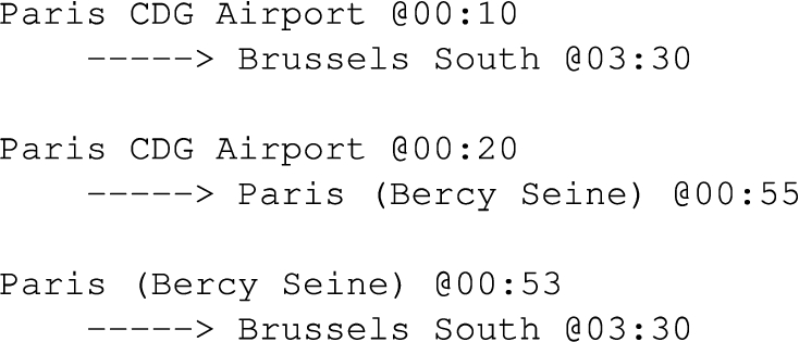
Listing 4.
Example of a cluster in EU-Flixbus. Given the long duration of the two connections departing from France to Brussels South, when the connection between the two french stops takes place, the other two connections are still happening, therefore a cluster (triangle) can be formed in the graph
Lastly, we see that the values for average connection duration range from 1.37 minutes of Chicago-CTA to 133.05 minutes of EU-Flixbus. This is expected, since urban networks normally have shorter connection durations compared to nation-wide or international networks such as Thailand-Greenbus and EU-Flixbus.
5.Evaluation
To support efficient pt data publishing and real-world practical use cases such as route planning, it is fundamental to achieve high performance for query processing. Performance in this case refers to the query response time (i.e. the time elapsed since a client sends a query request until it obtains a response). Therefore, we need to understand the factors that influence performance and the api design aspects that could be adjusted to optimize them. One of the aspects that can be controlled on lc systems, is the lc data fragment (document) size, in terms of the maximum number of connections they can contain. In previous work [17], we established arbitrary time window ranges (e.g. 10 minutes) per document, aiming to have lc documents of reasonable size to be transmitted to clients over http. However in practice, this resulted in a wide range of lc document sizes, which in turn translated to unpredictable query evaluation performance. This is due to pt networks normally exhibiting significantly higher amount of connections during peak hours, which also increase proportionally to the number of trips that take place on the network. For this reason we opted for establishing a (configurable) fixed size for lc documents, given by a maximum number of connections allowed per document. This results in more stable document response times over http and thus more predictable route planning performance. Determining the size of lc documents takes us to our first research question and hypothesis:
– RQ1: Is there an optimal data fragment size for maximizing route planning query performance of a pt network modeled and published as Linked Connections?
– H1: There is an optimal lc data fragment size for pt networks that renders the highest route planning evaluation performance.
This hypothesis comes from considering that bigger fragments will increase response times and processing effort for individual requests, and smaller fragments will require more http request-response cycles, both cases resulting in poorer overall query evaluation performance. Therefore, finding the optimal lc document size (max number of connections per document) of individual pt networks is an important design aspect for lc systems, but it does not provide a complete picture of the principles that guide better query performance. Finding a generalized solution that maximizes query performance when publishing lc, requires determining the patterns present when high performance is achieved. For this we observe the properties of the pt networks themselves, aiming on finding the conditions that determine better route planning performance. This takes us to our second research question and hypothesis:
– RQ2: Is there any correlation between route planning query performance over lc-based data interfaces and the topological properties of pt networks graphs in space-of-stops?
– H2: A lc interface gives a better performance for route planning queries, when publishing pt networks with certain topological values of size, K, D, C and
The main goal of lc is to achieve a reasonable trade-off between pt data publishers and consumers in terms of data integration and query processing efforts, that is targeted (but not limited) to route planning use cases. Our approach aims on improving the cost-efficiency of computational resources for pt data publishers by keeping simple server interfaces providing highly cacheable data responses. This design moves the responsibility of query execution to the clients, but it also provides them with a higher querying flexibility, i.e., clients are able to independently customize the query process and adjust it to their particular needs. In previous work [17], we observed that a lc interface does provide a better use of computational resources on the server-side and similar response times for route planning query solving, at the cost of an increased bandwidth use (3 orders of magnitude higher). However, that evaluation was done against a traditional server-side setup, which was only an adaptation of our client-side algorithm (csa) implementation published through an origin-destination API. Moreover, the comparison was made considering only one transport network, which does not allow to draw generalized conclusions. For these reasons, in this work we compare the cost-efficiency of lc, against the established and widely used pt route planning solution OpenTripPlanner. We consider 22 real and heterogenous pt networks and also evaluate the added costs of our extensions to the lc approach for publishing live and historical pt data. This takes us to our third and final research question and hypothesis:
– RQ3: What are the relative cost-efficiency and performance of lc-based data interfaces compared to the traditional pt route planning engine OpenTripPlanner?
– H3: lc interfaces achieve better cost-efficiency regarding server-side resources and offer an average route planning query performance in the same order of magnitude as the one offered by OpenTripPlanner.
To tackle these research questions, we performed empirical evaluations using the 22 real-world pt networks described in Section 4, where we (i) fragmented their corresponding lc collections and measured the performance of route planning queries with different fragments sizes; (ii) contrasted the measured network graph properties (size, average degree, density, clustering coefficient and average connection duration) of each pt network against their best measured route planning performance; and (iii) compared the (live and historical) route planning performance against OpenTripPlanner, while measuring server-side CPU and RAM use for an increasing amount of concurrent clients. Next we describe in detail the experimental protocols followed for each evaluation.
5.1.Preliminaries
We ran the experiments on one machine acting as server and one or more machines acting as clients. All machines had identical characteristics: 2x Quad core Intel E5520 (2.2 GHz) CPU with 16 threads and 12GB of RAM.
One important variable to consider, is the latency of the network. Given that we measure query response times, which largely depend on the amount of required http request-response cycles, network latencies may have a significant impact in particular for smaller fragmentation sizes, for which large number of requests are usually needed. However, latency in real scenarios is highly heterogeneous and depends on multiple factors (e.g., geographical location, network traffic and bandwidth) [6], making it difficult to predict reference values for it. Therefore, we perform our evaluations in a local network to eliminate the influence of variable latencies on the results. We deem out of scope for this paper, investigating how latencies may impact measured optimal fragment sizes. Our results may be considered as a reference point that could be adjusted when expected latencies are known in advance. For reproducibility and transparency, we made available the original data sources, query sets, tools and obtained results of these evaluations.2727
Two main tasks were completed before running the experiments, namely generating multiple fragmentation sets with varying size and producing a route planning query set for each considered pt network. We describe next how were these tasks completed.
5.1.1.Fragmenting Linked Connections
The steps taken to produce the fragmentation sets are as follows:
Generate Linked Connections We converted the pt networks to lc from gtfs data sources found on the Web as open data.2828 For this we used the gtfs2lc Node.js library.
Busiest day We looked for the busiest day of every pt network, by counting the number of connections present on each day. The busiest day acts as a representative subset of the planned schedules, given that for any other day, route planning algorithms will need to process less data to answer queries. We also made the assumption that in practical scenarios, most pt route planning queries will be normally evaluated within the span of one day. This assumption is derived from observing that most of the PT networks cease operation through the night, with a few exceptions. For example EU-Flixbus has several trips that go over midnight. In such cases, we included the data of all trips going over midnight for the busiest day of every network.
Smallest fragment possible Fragmentation of lc collections is driven by a configurable maximum number of connections allowed per document. However, a fragmentation cannot be arbitrarily small, because pt networks in lc systems have a lower bound of connections per document. This lower bound is determined by the maximum number of simultaneous connections in the smallest time interval possible in the schedules. In other words, connections sharing the same exact departure time, cannot be fragmented across different lc documents as this would break the indexing mechanisms that lc systems rely on. All of the 22 evaluated pt networks provide departure times with a resolution of one minute, therefore, we could determine the smallest possible fragment, by looking for the busiest minute, i.e., the maximum number of simultaneous connections in one minute. This lower bound gave us the minimum fragmentation size for every pt network. For example, it would not be possible to apply a fragmentation of 10 connections per document, for a pt network whose lower bound is 350 connections, without breaking the time-based index.
Fragmentation sets Knowing the lower bound, we proceeded to fragment the lc collections starting from their lower bound and progressively increasing the number of connections per fragment. We used fixed sizes of 10, 50, 100, 300, 500, 1,000, 3,000, 5,000, 10,000, 20,000 and 30,000 connections per fragment; since smaller pt networks have a low total number of connections, we stopped fragmenting the collections when the fragment size reached the size of the entire collection. We used these fragmentation sets of each pt network to measure and compare route planning query performance.
5.1.2.Route planning queries
Performance of route planning query evaluation not only depends on how the data is structured and published but also on the type of queries that need to be processed. The literature defines different classes of problems for the route planning use case that involve a varying number of variables. To minimize the number of variables that may influence our performance measures, we selected the simplest type of problem, namely the Earliest Arrival Time (eat) problem. We focused our evaluations on this particular problem only, considering that in the literature, more complex route planning scenarios are often addressed as extensions of the eat problem. Therefore optimizing our approach to handle eat queries would consequently improve also the performance of more complex route planning query processing over lc interfaces. The goal in the eat case, is to find the journey with the shortest travel duration between origin and destination, given a minimum departure time. Processing of these queries focuses only on optimizing the arrival time, disregarding other common variables such as maximum number of transfers or transportation modes.
In our test case, transfers are possible but constrained only to a maximum walking time of 10 minutes at an average speed of 3 km/h (500 meters). Transfers are computed on the fly using the Haversine formula2929 and are modeled as additional connections. We assumed a restricted walking scenario based on a realistic heuristic to avoid the complexity of unrestricted walking calculations having an influence in the results. eat queries can be processed easily over lc interfaces via the csa algorithm. The algorithm can perform a single scan over the lc collection until it finds a complete journey (if any), which is guaranteed to be the earliest arrival thanks to the chronological ordering of the lc collection.
Query selection for each pt network in our evaluation was performed at random, for origin-destination stop pairs at any time of the day. We randomly generated 100 (solvable) queries for each network. We counted the number of connections that csa had to process to evaluate each individual query and called this the number of Scanned Connections needed by the Query (scq). The counting was done within csa’s execution loop to avoid fragment sizes having an influence on the count.
Table 3
Average number of connections (
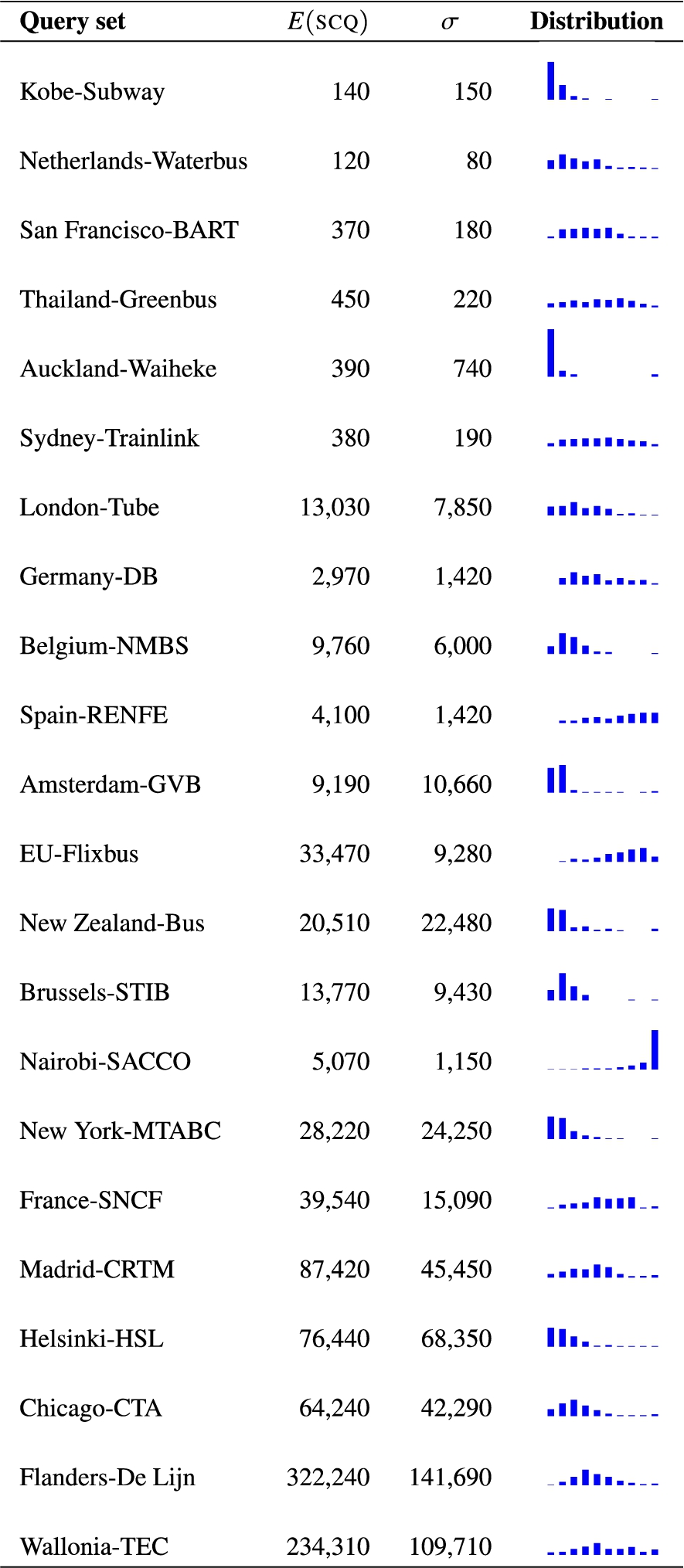
Table 3 shows a summary of
5.2.Experiment 1: Optimal lc fragmentation size
In this first experiment we deployed an instance of the lc Server3030 in one of our test machines. We configured it to publish the planned schedules of every pt network, using the predefined fragmentation sizes. We enabled only one network with one fragmentation at a time. For the client we deployed in a different test machine, one instance of Planner.js3131 and configure it to replay (3 times) each respective query set against the lc Server instance. We registered the average query response time of Planner.js for every pt network, using each predefined fragmentation size.
5.3.Experiment 2: Correlation of graph metrics and query performance
To analyze the potential correlations between the intrinsic graph characteristic of each pt network and their route planning query performance, we first measured the defined set of graph metrics (Section 4) for each of the considered pt networks. The calculation of the metrics was performed over the
The correlation analysis was made by calculating the Pearson Correlation Coefficient (r), Covariance (
5.4.Experiment 3: Cost-efficiency of the lc approach
For measuring the relative cost-efficiency of our approach, we performed two main evaluations: (i) lc Server vs OpenTripPlanner with planned schedules; and (ii) lc Server with live and historical schedules vs lc Server with planned schedules only. We were not able to directly compare our approach with OpenTripPlanner handling live and historical data because OpenTripPlanner does not support route planning querying based on historical data (e.g., calculate a route from A to B considering the schedule reports of 30 minutes ago is not supported). In the case of live data, we had access to the gtfs-realtime stream containing live schedule updates from the Belgium-NMBS pt network, but OpenTripPlanner failed to integrate this data source with errors regarding the integrity of the data. Next we describe these two experimental setups.
5.4.1.lc vs OpenTripPlanner
For this evaluation we deployed instances of the lc Server and OpenTripPlanner on independent and identical test machines acting as servers. We restricted both instances to run in a single CPU core. Our goal is to observe how fast CPU usage increases when the number of clients scales. Therefore the results do not reflect the full capacity of the test machines. In a production environment, the applications would be horizontally scaled to completely use the machine’s hardware capacity and possibly set behind a load balancer to improve the overall performance. We also used a server-side http caching system (NGINX) acting as a reverse proxy for the lc Server deployment.
The deployments were tested with 16 out of the 22 pt networks. We were not able to instantiate OpenTripPlanner for some of the country and continent-wide transit networks, namely Spain-RENFE, France-SNCF, Germany-Deutsche Bahn and EU-Flixbus given that the memory requirements exceeded the hardware capabilities (12GB) of the test machines. For OpenTripPlanner is mandatory to provide the OpenStreetMap road network of the geographical area over which pt routes will be calculated, which exceeds 12GB on large geographical areas, even after filtering for road data only. Additionally, OpenTripPlanner failed to load the road network of New Zealand, which prevented us to evaluate Auckland-Waiheke and New Zealand-Bus networks.
On the client side, we used the http benchmarking tool autocannon3636 to generate an increasing amount of concurrent clients over OpenTripPlanner’s route planning rest API. In the same way, we run an instance of Planner.js next to an increasing amount of autocannon clients (each running on independent threads in one or more test machines) over the lc Server. We created loads of 1, 2, 5, 10, 20 and 50 concurrent clients replaying the respective query sets 3 times, while recording CPU and RAM use on the server and the query response times on the clients.
5.4.2.Live and historical data with lc
In this evaluation, we deployed an instance of the lc Server publishing the planned, live and historical schedules of the Belgium-NMBS network. We recorded the real schedule updates emmited on 19-07-20213737 and the gtfs-realtime updates,3838 which are replayed within our experimental setup. We performed 3 different tests, with an increasing amount of Planner.js + autocannon instances (1, 2, 5, 10, 20 and 50), replaying 3 times the query set for this network as follows: (i) Planner.js executed the query processing based on the last known state of the schedule, while the lc Server kept on processing updates (every 30 seconds) from the gtfs-realtime stream; (ii) Planner.js executed the query processing based on historical connections from 1 hour before the query’s departure time, while the lc Server kept on processing new schedule updates; and (iii) Planner.js executed the query processing based on the planned schedule only as a baseline reference. In every test we measured CPU and RAM use on the server-side and registered the query response times of Planner.js.
6.Results
In this section we present the measurements obtained during our evaluations. We first present the results of route planning query performance using different fragmentation sizes. Afterwards, we contrast each of the considered metrics against the query performance results and present the calculated statistical correlation measures. Lastly, we show the measured results on cost-efficiency in terms of server-side resources use and query response time for our solution and OpenTripPlanner. We also show the additional costs measured for our solution, when publishing live and historical pt data.
6.1.Experiment 1: Optimal lc fragmentation size
Figure 6 presents an overview of the results obtained from the route planning performance evaluation, over different sets of lc data fragmentation.
Fig. 6.
Average response time of route planning queries (ms) vs fragment sizes (connections) for each pt network. pt networks with similar total number of connections (see Table 2) are grouped together to facilitate visualizing the results. We labeled the lowest point of each curve where best performance is achieved. Axes use logarithmic scales.
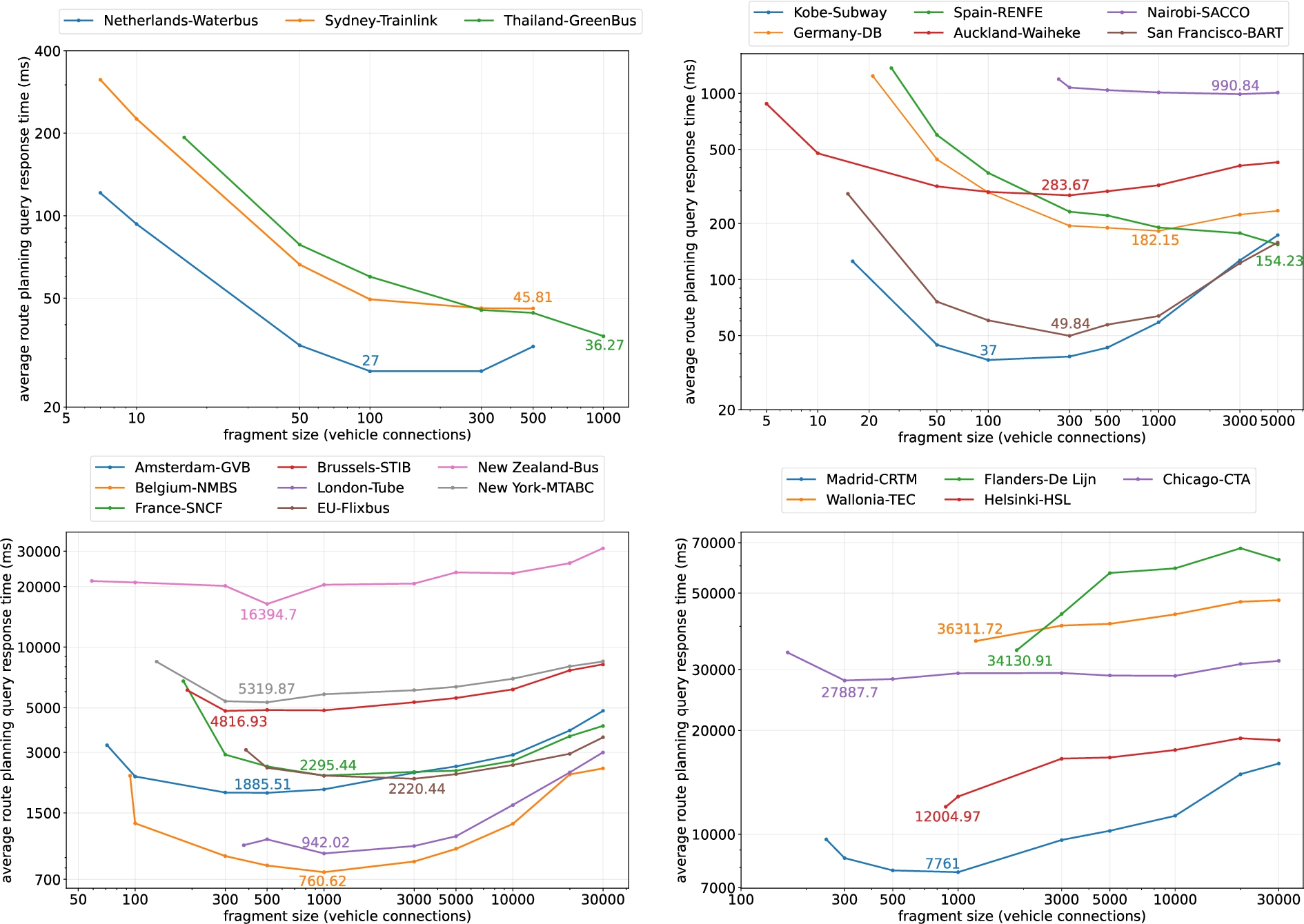
The top left plot in Fig. 6, shows the results for the three smallest networks in terms of total connections (<1,100). Fragmentation was only possible until 500 connections/fragment for Netherlands-Waterbus and Sydney-Trainlink, and until 1,000 connections/fragment for Thailand-Greenbus. Bigger fragmentation for these networks would mean that the entire collection of connections would fit in only one fragment. Netherlands-Waterbus shows its best performance (27 ms) with a fragmentation of 100 connections/fragment. Sydney-Trainlink’s best performance (45.81 ms) was achieved with 500 connections/fragment, while Thailand-Greenbus (36.27 ms) was achieved at 1000 connections/fragment. Netherlands-Waterbus shows faster query responses compared to both Sydney-Trainlink and Thailand-Greenbus, which may be explained by the higher number of connections per query (
The top right plot in Fig. 6, brings together 6 different networks with total amounts of connections ranging between 5,000 and 8,000. Optimal fragmentation values are different for each network, except for Auckland-Waiheke and San Francisco-BART both with 100 connections/fragment. Despite having the same optimal point and similar amout of connections, they show a significant difference in terms of response time, with 283.67 and 49.84 ms respectively. Referring to Table 2, we can see that both networks differ significantly for K and D: San Francisco-BART(
In the bottom left plot of Fig. 6, we have a set of 8 pt networks with total amounts of connections ranging between 51,000 and 350,000. Most networks show an optimal fragmentation of 500 and 1,000 connections/fragment, with the exceptions of Brussels-STIB and EU-Flixbus with 300 and 3,000 connections/fragment respectively. New Zealand-Bus shows significanlty worse performance than the rest of the networks, followed by New York-MTABC and Brussels-STIB. Comparing them to the more performant Belgium-NMBS and London-Tube we can see that the less performant networks have higher amount of stops and a lower values for K and D.
Lastly, on the bottom right plot in Fig. 6 we see the results for the remaining 5 networks. These are the biggest networks in the set with total number of connections ranging from 689,000 to 1.2 million. In this case we see a generally degraded performance for all networks. Only Madrid-CRTM and Chicago-CTA show an optimal fragmentation point on 1000 and 300 connections/fragment respectively. The rest of the networks show their best performance with their smallest fragmentation possible which only degrades further with bigger fragments.
Fig. 7.
Measured average response time in milliseconds for the fragmentation that rendered the best performance for each pt network. X-axis uses a logarithmic scale.
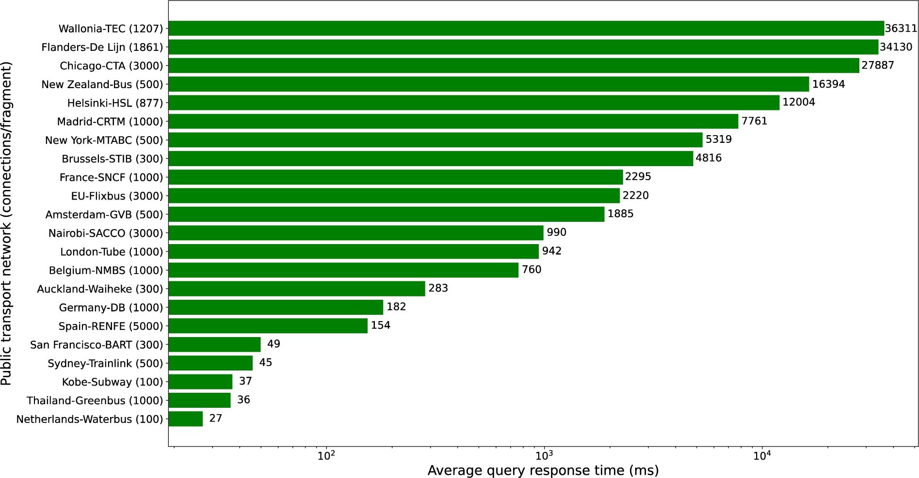
In Fig. 7 we present the average query response times, measured using the optimal fragmentation found for each network (as seen on Fig. 6). An annotation can be seen next to every network’s bar indicating the average time (in ms) needed to answer the queries of the query sets. At first glance we can see that bigger networks in terms of total number conenctions and stops are less performant. However, London-Tube and New Zealand-Bus stand as execptions on both sides of the spectrum for this trend. London-Tube is a relatively big network (321,000 connections) with subsecond performance and New Zealand-Bus is a medium size network (153,000 connections) with much worse performance (16.3 s) compared to networks of similar size.
6.2.Experiment 2: Correlation of graph metrics and query performance
Results on how the different graph network metrics relate with route planning query performance can be seen on Fig. 8. Correlation measures (Pearson Coefficient,3939 Covariance4040 and Coefficient of Determination4141) of each metric are also shown in Table 4.
Fig. 8.
pt network metrics compared with route plannning query performance. Each sub-graph compares one of the metrics to the best query evaluation performance measured for each network (see Fig. 7.) Axes are set in logarithmic scale.
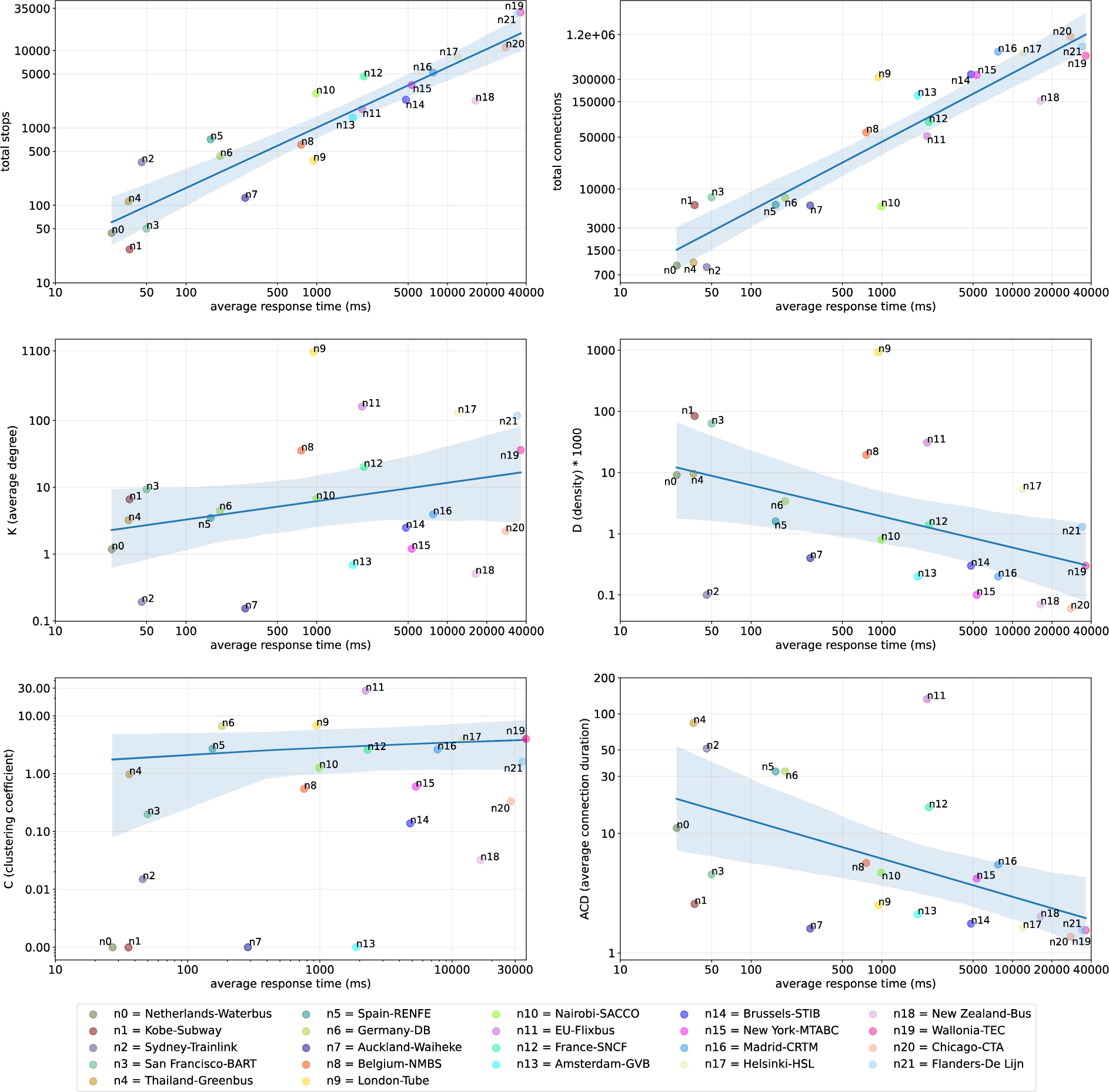
Table 4
Correlation measurments for each graph metric vs route planning query performance. The measured correlations the Pearson Coefficient (r), Covariance (
| r | |||
| 0.9225 | 9.2e7 | 85.29 | |
| connections | 0.8055 | 30.5e8 | 64.88 |
| K | −0.0528 | −13.5e4 | 0.27 |
| D | −0.1499 | −33.6e4 | 2.24 |
| C | −0.0569 | −3.7e3 | 0.32 |
| −0.2811 | −10.4e4 | 7.90 |
The correlation measures (Table 4) related to number of stops (
Weak and inverse correlations can be observed for both D (center right) and
Lastly, no correlation can be seen for the cases of K and C, both with Pearson coefficients close to zero and showing high disperssion for query performance.
6.3.Experiment 3: Cost-efficiency of the lc approach
Next we present the results of our two experimental setups for measuring the cost-efficiency of our solution.
6.3.1.lc vs OpenTripPlanner
In Fig. 9 we present the server-side CPU and RAM use for both OpenTripPlanner and the lc Server, while supporting route planning query solving for an increasing amount of concurrent clients. We can see that CPU use for OpenTripPlanner increases proportionally to the number of clients and is also related to the size of the networks (in terms of stops), with bigger networks consuming more processing capacity. The lc Server presents a stable CPU consumption as the number of clients increases, with all networks requiring around 20% of the processor capacity.
In the case of RAM consumption, both OpenTripPlanner and the lc Server remain constant for all networks regardless of the amount of concurrent clients. For all networks, the lc Server does not exceed 10% of RAM use, while OpenTripPlanner reaches up to 70%. In general, the lc Server consumes less CPU and RAM resources and shows a better scalability than OpenTripPlanner.
Fig. 9.
CPU (left column) and RAM (right column) usage under an increasing amount of concurrent clients of OpenTripPlanner and the lc Server for 16 different pt networks. Each row groups 4 networks of similar amount of stops, with smaller networks at the top and bigger networks at the bottom. Dotted lines represent measurements for OpenTripPlanner and continous lines represent measurements for the lc Server.
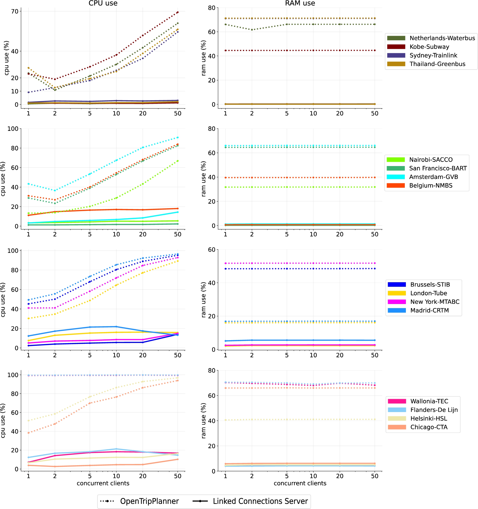
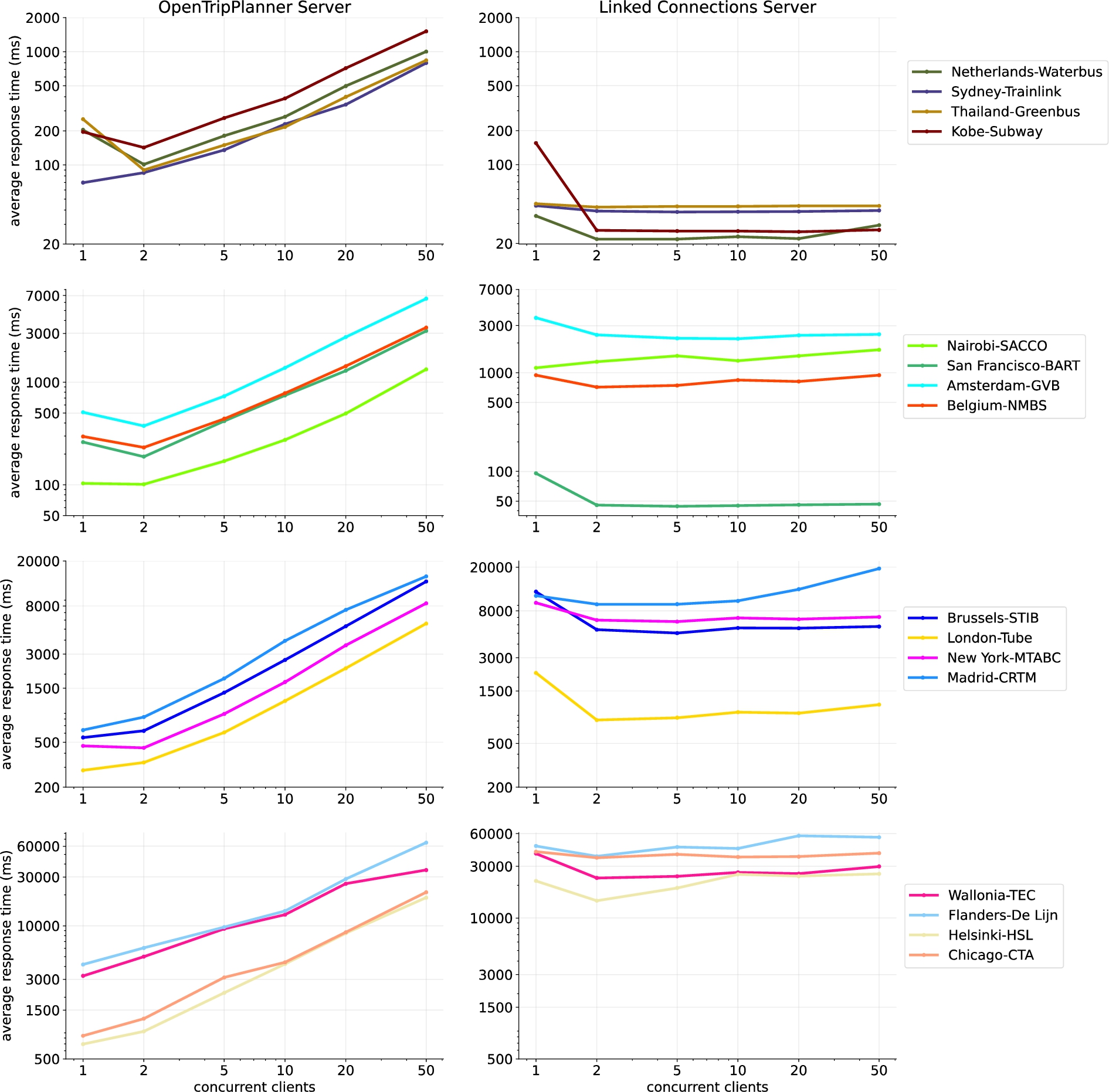
Figure 10 presents the obtained results on average query response time for both OpenTripPlanner and the lc Server. The average query response time increases proportionally to the number of concurrent clients for OpenTripPlanner, which reflects the behaviour observed in Fig. 9 regarding CPU use. Response times over the lc Server are also aligned to its CPU use and remain relatively stable when the number of clients increases. In terms of absolute numbers, the lc Server completely outperforms OpenTripPlanner for the smallest pt networks of the set (first row) and San Francisco-BART (second row). In contrast, OpenTripPlanner significantly outperforms the lc Server for the biggest networks (last row), although response times become similar with 20 and 50 concurrent clients. In the case of middle size pt networks, OpenTripPlanner shows better perfomance for low amount of concurrent clients (<10). However, the lc Server shows similar or in some cases better performance for higher amount of concurrent clients (⩾10), as is the case of Belgium-NMBS, Amsterdam-GVB, London-Tube, Brussels-STIB and New York-MTABC.
Fig. 10.
Average route planning query response times for OpenTripPlanner (left column) and the lc Server (right colum) with an increasing amount of concurrent clients. Each row groups 4 networks of similar amount of stops, with smaller networks at the top and bigger networks at the bottom.
6.3.2.Live and historical data with lc
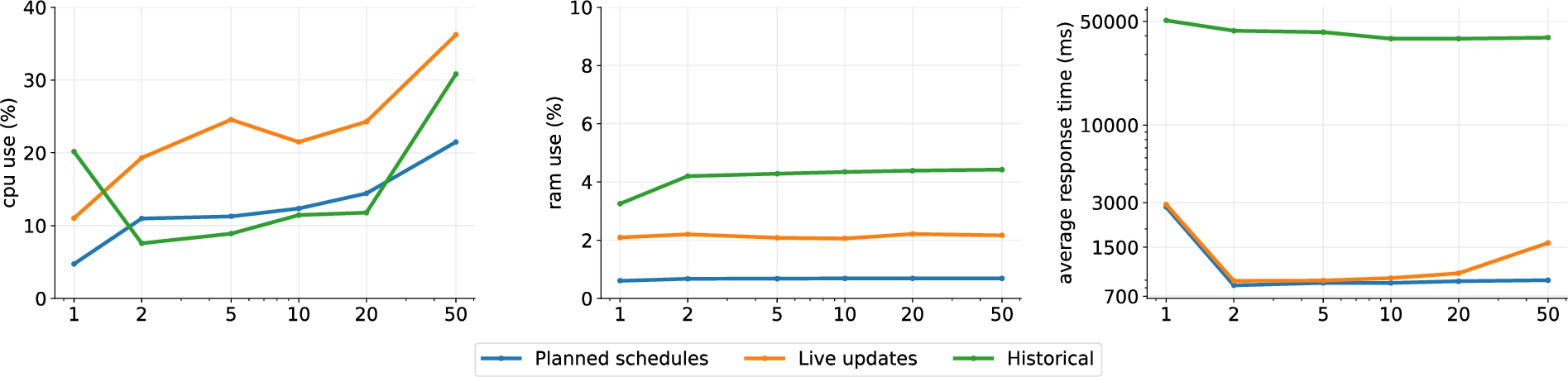
Figure 11 presents the CPU (left) and RAM (center) use, and the average response time of route planning queries (right) of the lc Server when publishing planned schedules only, live schedules updates and historical schedules. In terms of CPU consumptions we see similar behavior for all configurations ranging between 5–38% and having the live updates setup as the most demanding one. RAM consumption remains stable as the number of clients increases and has the historical setup as the most demanding with 4%. In terms of query response times, both planned only and live updates configuration perform similarly. Query response times over historical data on the other hand, show a significant performance degradation, being 50 times slower.
Fig. 11.
On the left plot is the CPU usage of the lc Server publishing planned only, live updates and historical pt schedules under an increasing amount of concurrent clients. The center plot shows the RAM use for each publishing configuration. The left plot shows the average route planning query response times for each publishing setup of the lc Server.
7.Discussion
We addressed the problem of publishing live and historical pt data in a cost-efficient way. For this, we defined a reference architecture and implementation that extends the lc approach for publishing planned schedules. Our approach handles pt schedule requests that include live updates efficiently, and is capable of providing the historical stream of events that ocurred on a pt network. This constitutes an important innovation and contribution that may be used to support for example machine learning-based applications, able to accurately predict the future state of a network.
We also studied how our approach could be used to support route planning use cases and how data fragmentation impacts the performance of query evaluation. We measured different topological characteristics (in space-of-stops) of the 22 real pt networks considered in this paper and anlayzed their correlation with route planning query response time, aiming on understanding the factors that drive better or worse performance. Additionally, we compared the cost and performance or our approach with the traditional and widely popular solution OpenTripPlanner. Furthermore, me measured the introduced costs of our solution when publishing live updates and historical schedules compared to only publishing planned schedules. Next we elaborate on these results obtained during each of our experimental setups.
7.1.Optimal lc fragmentaion size
Our evaluation showed that for each pt network the best performance is achieved with a certain fragmentation size. This constitutes an important finding for data publishers that may be considered when designing pt data apis. Results also showed that for most networks, either increasing or decreasing the fragmentation size, degrades performance of route planning query evaluation. Smaller fragmentation than the optimal point, degraded performance due to the higher number of http request-response cycles needed with smaller fragments. Larger fragment sizes require clients to perform fewer cycles but need to process increased number of irrelevant connections for each query. Exceptions occured on some of the smallest networks having their optimal fragmentation at the biggest possible size, and for some of the biggest networks having their optimal fragmentation at the smallest possible size. One particular case can be observed for Spain-RENFE, a medium size network (in terms of stops) whose optimal fragment size was found on its biggest fragmentation possible (5000 connections/fragment). Such behavior of Spain-RENFE may be explained by a high value of
Another important finding of this evaluation is the fact that for several networks, this approach results impractical for real scenarios. Response times on the order of seconds and even tens of seconds per query are unacceptable for user-oriented applications. However is important to mention that for this particular evaluation we did not use any form of caching (server nor client-side), which is one of the fundamental features of publishing pattern-based fragmented datasets. Our goal was to study the impact that data fragmentation has on query performance. Different fragmentation setups influence the effort that server-side data interfaces make to respond to data fragment requests, as well as the effort made by client-side route planners for evaluating queries. We wanted to quantify these efforts and both server and client-side caches would have hidden the effect of any fragmentation. A server-side cache frees the data interface of having to retrieve, parse and format data fragments more than once across queries, while a client-side cache makes unecessary to request data fragments fetched on previous queries. Therefore, the results of this evauation may be considered as worst-case scenario values and it could be expected that in practice query response times will be improved.
7.2.Correlation of graph metrics and query performance
When looking at the topological properties of every pt network and the calculated correlation indicators (Table 4), we observe the existence of a strong and direct correlation between the size of the network, both in terms of stops and connections and the query response time. This is not a surprising result since is expected that in the presence of more connections, route planning algorithms would need to process more data during query evaluations. Yet, it is interesting to look into individual cases that differ significantly (for better or worse) in query evaluation performace, compared to networks of similar characteristics. Examples of this atypical behavior in the case of total number of connections are London-Tube or Belgium-NMBS for better performance and Nairobi-SACCO or New Zealand-Bus for worse performance.
Weak and inverse correlations are observed for the cases of density (D) and average connection duration (
Lastly, we observe no correlation for the cases of average degree (K) and clustering coefficient (C), both with Pearson’s coefficients close to zero, which suggests that these properties do not influence route planning performance.
7.3.Cost-efficiency of the lc approach
We considered OpenTripPlanner as a traditional route planning reference solution, to compare against our proposed approach. However, as remarked in Section 5.4, we were not able to compare against OpenTripPlanner considering live and historical data. Thus, we performed the comparison with OpenTripPlanner with planned schedules only and for live and historical data, we measured the added costs of our proposed extensions to the lc approach.
7.3.1.lc vs OpenTripPlanner
A first sign of the better cost-efficiency of lc was evident when the RAM requirements of OpenTripPlanner exceeded the capabilities of our test servers (12GB) for offering route planning services over country and continent-wide networks. This is required by OpenTripPlanner to pre-calculate the walking transfers graph that will be used for solving route planning queries. In our approach, Planner.js calculates walking transfers on the fly, either based on Haversine distance or also relying on OpenStreetMap road network data [14], which prevents us having to preload full road networks in memory.
Our evaluation results further confirmed the lc approach as a more scalable and cost-efficient alternative for publishing pt schedules. The lc Server uses significanlty less CPU and RAM resources on the server-side and remains stable when the number of clients increases. In contrast OpenTripPlanner’s CPU use increases proportionally to the amount of clients. OpenTripPlanner’s RAM use remains stable, regardless of the number of clients, but is higher for every network when compared to the lc server. For data publishers wanting to support route planning services, this means that more expensive servers will be needed with OpenTripPlanner than with the lc Server.
Claiming superior cost-efficiency of our approach for route planning use cases, requires us to look not only to the server’s resource consumption but also into the query solving performance. Lower resource consumption on the server-side does not add value if query performance is significantly compromised. However, our evaluation results showed that for some of the considered networks (Netherlands-Waterbus, Sydney-Trainlink, Thailand-Greenbus, Kobe-Subway and San Francisco-BART), the lc server also renders better query performance with any amount of concurrent clients. Other networks such as Belgium-NMBS, Nairobi-SACCO, Amsterdam-GVB and London-Tube initially render better performance on OpenTripPlanner with few clients, but eventually show similar or better performace on the lc Server when the number of clients increases. This is an important achievement for the lc approach that confirms its applicability in real world scenarios, having more than half the networks (9 out of 16) that we were able to compare, showing similar or better performance than OpenTripPlanner.
On the other hand and as already observed in the results of our first experiment (Section 6.1), for the rest of the networks (Brussels-STIB, New York-MTABC, Madrid-CRTM, Wallonia-TEC, Flanders-De Lijn, Helsinki-HSL and Chicago-CTA) the lc Server does not provide a level of performance that is acceptable for practical scenarios. For the same networks, OpenTripPlanner gives significanlty better performace under low load only, but with horizontal scaling it can provide a (costly) production-ready solution. The common denominator observed among the pt networks for which the lc Server provides superior performance, is a relatively low amount of stops (<1000). This means it would be possible for example, to create geospatially meaningful sub-networks that could provide similar performance as the one obtained for the smaller networks in this evalaution.
Another important aspect to consider in our approach, is the trade-off of server’s computational cost vs client’s computational cost, implementation complexity and bandwidth (measured in previous work [17]) requirements. A lc client needs to perform data fetching, hypermedia controls interpretation and route planning algorithm execution tasks, to calculate a route alternative. In contrast, a traditional route planning client only needs to send and process a single API request, which already returns a fully formed route (if any). Implementation complexity of an lc client, may be handled by relying on software modularization. For instance, our client application Planner.js can also be used as a library by other applications, both on client- and server-side (in Node.js environments). However, bandwidth and computational resource requirements may be execisve for practical use, for example in mobile application environments. This limitation could be mitigated by running a lc client as part of the server infrastructure of a pt data provider. The lc client may in turn, be wrapped within a traditional origin-destination api, that can be consumend by mobile/browser client applications. In this way it is possible to take advantage of the best characteristics of both, fully server and client side processing architectures.
7.3.2.Live and historical data with lc
When it comes to live data publishing, our approach is fundamentally different to traditional data interfaces, regarding where data integration of planned and live schedule updates takes place. Traditionally, data publishers expose a stream/feed api of live data updates using siri or gtfs-realtime data models. Besides the request limitations that these apis normally impose to avoid server overloads, this also transfers all the computational burden of data integration and reconciliation to data reuser applications. Reuser applications need to perform frequent requests to such apis to keep their internal databases up to date, and thus reflect the new schedule changes. In contrast, our approach performs such integration in an cost-efficient way on the server-side api, as reflected on the results obtained in our evaluation (Section 6.3.2). Publishing live schedule updates doubles the CPU use on the server-side compared to just publishing planned schedules. RAM use also increases going from 0.5 to 2%. These increases can be explained by the frequent fetching and processing of schedule updates that takes place on the server. Yet, even under a load of 50 concurrent clients, the CPU use does not go over 40%.
More importantly, query performance remains unaltered, only showing a not negligible increase (from 800 ms to 1500 ms) with 50 concurrent clients. This is due to the in-memory AVL tree data structure, introduced by our approach, that allows for fast and efficient data responses. This added to the planned schedule fragmentation approach of lc, constitutes a cost-efficient approach for publishing of dynamic pt schedules directly from the source, while freeing data reuser applications from expensive data reconciliation tasks.
When looking into pt historical data we can see that is not available for most pt networks as open data on the Web. Older versions of planned schedules are sometimes available for some pt networks, but historical records of data updates are usually not published as open data through traditional apis. Our approach enables access to the historical records of previous versions of planned schedules and also to the update stream flow as it occured. More importantly, it also defines a query interface for this data, built using a standard time-based content negotiation protocol over http, which provides access to historical data with high granularity.
Considering the added costs of publishing historical data through our approach, we can see that there is no considerable increase on server-side resource consumption (CPU and RAM), compared to just publishing planned schedules. However, we see a significant performance degradation (50 times slower) for route planning query performance. This is due to the data reconciliation processes that take place in the lc server, to merge static and live update records, which can be time consuming depending on the amount of records available. Also due to the additional http 302 redirections that occur following the implemented pattern of the Memento protocol. Additional optimizations are possible, e.g., implementing more efficient indexes for (time) range queries within the lc Server and using a redirection-less Memento pattern.
Despite the performance limitations for requesting historical schedules with high granularity, we highlight that our approach puts forward a low-cost alternative to publish queryable pt historical data as open data. To the best of our knowledge, our approach is the first open source alternative to offer access to historical records, as we see that established and traditional solutions, such as OpenTripPlanner do not provide any means to access these type of data.
8.Conclusions and Future Work
Our work stands as a contribution for the pt domain as a cost-efficient data publishing alternative that includes live schedule updates and access to granular historical data. We propose a different approach on how live data is published, compared to traditional apis, that facilitates data reuse for client applications without sacrificing cost-efficiency on the server-side. At the same time we enable data publishers to also share historical data, which still remain largely unavailable.
The use of semantic Web technologies establishes a framework for data interoperability on the pt domain. Ideally, every pt operator would publish and maintain stable identifiers for their resources such as stops, routes and connections. This way, semantic interoperability starts at the source, where all derived datasets can reuse the same identifiers. This approach not only semantically models the fundamental entities and concepts of pt schedules and its updates, but also the interfaces that give access to the data. It relies on the Web infrastructure to model entire datasets as collections of http resources, while including metadata that semantically describes the access patterns to traverse the collection and find more relevant data. This constitutes an important contribution for the pt domain and also sets an example that may be applied on different domains or use cases.
Being a Linked Data-based approach, a lc interface not only enables client applications to perform route planning-related calculations, but could also allow them to apply (on their own premises) other types of querying approaches (e.g., SPARQL) to support novel use cases. A client application able to interpret the hypermedia controls of lc data fragments could traverse the lc collection to solve a federated SPARQL query (for example with Comunica [52]) to find departing vehicles from stops having images (wdt:P184242) available in Wikidata (e.g. Gent-Sint-Pieters4343). We hope an approach such as Linked Connections inspires pt organizations to publish their raw base data as a back-bone for creating new and innovative applications.
Considering the importance of query evaluation performance for supporting practical use cases, we evaluated our approach looking into understanding the factors that drive high performance and how api design can be adjusted to achieve it. With regards to our first research question RQ1, we conclude to accept its associated hypothesis H1, which constitutes an important result that highlights the importance of adapting api data structures to improve the performance of use case-specific query evauation. Regarding research question RQ2, we also conclude to accept its associated hypothesis H2. Results showed that size in terms of stops and connections is highly correlated to query evaluation performace. We could also see that density and average connection duration can also provide an indication of the expected performance. Additionally, we observed that an external factor as the number of scanned connections of expected queries could also guide api design as e.g., the size of data fragmentation.
An important finding of this work is the confirmation that our approach provides an acceptable performance to be used in practical scenarios for relativelly small pt networks (<1000 stops). It was also evident that larger networks still remain unfeasible to be published and used in practical scenarios using this approach. This was determined by looking at the measured response times in comparison to a state of the art solution such as OpenTripPlanner, during our evaluations related to research question RQ3 and its associated hypothesis H3. Results confirmed the superior cost-efficiency and scalability of our approach in all cases, despite the lower query performance of larger networks. More importantly, for smaller networks our approach gave as good as and even better query performace than OpenTripPlanner. Based on these results we may conclude to accept H3 for pt networks with less than 1000 stops.
These results may provide a reference guideline for data publishers to help balance the financial costs associated to open data publishing, wether they are required to do so by legal mandate or motivated by a business interest. The scalability evaluation results provide clear indicators of the amount of computational resources that would be needed to support a route planning service for a certain PT network, architecture and querying load. These could be then used to estimate practical financial costs on a certain cloud provider based on up to date pricing models and according to the capabilities and resources available to the data publisher. Yet, further studies can be made on cost estimation of (Linked Data) apis based on data source characteristics and expected queries.
Further research is needed to optimize use case driven query performance without compromising on cost-efficiency for both data publishers and reusers. On-going and future research is investigating alternative and additional fragmentation possibilities beyond time-based, such as geospatially [21]. The results shown in this paper are instrumental in that regard, as they also provide indications about network characteristics where higher performance can be expected and thus, how larger networks could be further fragmented so that individual sub-networks render acceptable query evaluation performance.
Notes
2 In 2017 Google announced having over 1 billion active users every month for Google Maps. https://www.theverge.com/2017/5/17/15654454/android-reaches-2-billion-monthly-active-users.
9 gtfs dumps from around the world: https://transitfeeds.com/, https://www.transit.land/.
29 Our implementation uses the haversine JavaScript library https://github.com/njj/haversine.
30 We used the swj-evaluation branch: https://github.com/linkedconnections/linked-connections-server/tree/swj-evaluation.
31 We used the swj-eval branch: https://github.com/openplannerteam/planner.js/tree/swj-eval.
39 Commonly represented as r: https://en.wikipedia.org/wiki/Pearson_correlation_coefficient.
40 Commonly represented as
41 Commonly represented as
Acknowledgements
We would like to thank David Chaves Fraga and Oscar Corcho for pushing us forward to write this paper.
References
[1] | Ably The Maturity of Public Transport APIs 2019, Technical Report, 2019, https://files.ably.io/research/whitepapers/the-maturity-of-public-transport-apis-2019-ably-realtime.pdf. |
[2] | G.K. Bailey, The Case for Open Data in Public Transport, UITP, 2020, https://www.uitp.org/news/the-case-for-open-data-in-public-transport/. |
[3] | H. Bast, D. Delling, A.V. Goldberg, M. Müller-Hannemann, T. Pajor, P. Sanders, D. Wagner and R.F. Werneck, Route Planning in Transportation Networks, CoRR (2015), arXiv:1504.05140. |
[4] | H. Bast, M. Hertel and S. Storandt, Scalable transfer patterns, in: 2016 Proceedings of the Eighteenth Workshop on Algorithm Engineering and Experiments (ALENEX), (2016) . |
[5] | M. Berkow, A.M. El-Geneidy, R.L. Bertini and D. Crout, Beyond generating transit performance measures: Visualizations and statistical analysis with historical data, Transportation Research Record 2111: (1) ((2009) ), 158–168. doi:10.3141/2111-18. |
[6] | D. Bermbach and E. Wittern, Benchmarking Web API quality, Revisited, Journal of Web Engineering 19: ((2020) ), https://journals.riverpublishers.com/index.php/JWE/article/view/5719. doi:10.13052/jwe1540-9589.19563. |
[7] | T. Berners-Lee, J. Hendler and O. Lassila, The Semantic Web, Scientific American 284: (5) ((2001) ), 34–43, http://www.sciam.com/article.cfm?articleID=00048144-10D2-1C70-84A9809EC588EF21. |
[8] | C. Bizer, T. Heath and T. Berners-Lee, Linked data-the story so far, International journal on semantic web and information systems 5: (3) ((2009) ), 1–22. doi:10.4018/jswis.2009081901. |
[9] | S. Boccaletti, V. Latora, Y. Moreno, M. Chavez and D.-U. Hwang, Complex networks: Structure and dynamics, Physics Reports 424: (4) ((2006) ), 175–308, http://www.sciencedirect.com/science/article/pii/S037015730500462X. doi:10.1016/j.physrep.2005.10.009. |
[10] | G.S. Brodal and R. Jacob, Time-dependent networks as models to achieve fast exact time-table queries, Electronic Notes in Theoretical Computer Science 92: ((2004) ), 3–15, Proceedings of ATMOS Workshop, 2003, http://www.sciencedirect.com/science/article/pii/S1571066104000040. doi:10.1016/j.entcs.2003.12.019. |
[11] | D. Chaves-Fraga, A. Antón, J. Toledo and Ó. Corcho, ONETT: Systematic knowledge graph generation for national access points, in: SEM4TRA-AMAR@SEMANTICS, (2019) . |
[12] | D. Chaves-Fraga, J. Rojas, P. Vandenberghe, P. Colpaert and Ó. Corcho, The tripscore linked data client: Calculating specific summaries over large time series, in: DeSemWeb@ISWC, (2017) . |
[13] | C. Chen, T. D’Alfonso, H. Guo and C. Jiang, Graph theoretical analysis of the Chinese high-speed rail network over time, Research in Transportation Economics 72: ((2018) ), 3–14, Long-distance passenger transport market, http://www.sciencedirect.com/science/article/pii/S0739885917303141. doi:10.1016/j.retrec.2018.07.030. |
[14] | P. Colpaert, B. Abelshausen, J.A.R. Meléndez, H. Delva and R. Verborgh, Republishing OpenStreetMap’s roads as linked routable tiles, in: The Semantic Web: ESWC 2019 Satellite Events, P. Hitzler, S. Kirrane, O. Hartig, V. de Boer, M.-E. Vidal, M. Maleshkova, S. Schlobach, K. Hammar, N. Lasierra, S. Stadtmüller, K. Hose and R. Verborgh, eds, Springer International Publishing, Cham, (2019) , pp. 13–17. ISBN 978-3-030-32327-1. doi:10.1007/978-3-030-32327-1_3. |
[15] | P. Colpaert, A. Llaves, R. Verborgh, O. Corcho, E. Mannens and R. Van de Walle, Intermodal public transit routing using Linked Connections, in: Proceedings of the 14th International Semantic Web Conference: Posters and Demos, CEUR Workshop Proceedings, Vol. 1486: , (2015) , ISSN 1613-0073, http://ceur-ws.org/Vol-1486/paper_28.pdf. |
[16] | P. Colpaert and J. Rojas, Open data sectors and communities: Transport, in: The State of Open Data: Histories and Horizons, African Minds, (2019) . doi:10.5281/zenodo.2677833. |
[17] | P. Colpaert, R. Verborgh and E. Mannens, Public Transit Route Planning Through Lightweight Linked Data Interfaces, W. Engineering, J. Cabot, R. De Virgilio and R. Torlone, eds, Springer International Publishing, Cham, (2017) , pp. 403–411. ISBN 978-3-319-60131-1. |
[18] | T. Davies, S.B. Walker, M. Rubenstein and F. Perini, The State of Open Data: Histories and Horizons, African Minds, (2019) . ISBN 9781928331957. |
[19] | D. Delling, J. Dibbelt and T. Pajor, Fast and exact public transit routing with restricted Pareto sets, in: Proceedings of the Twenty-First Workshop on Algorithm Engineering and Experiments, ALENEX 2019, San Diego, CA, USA, January 7–8, 2019, (2019) , pp. 54–65. doi:10.1137/1.9781611975499.5. |
[20] | D. Delling, T. Pajor and R.F. Werneck, Round-based public transit routing, in: Proceedings of the Meeting on Algorithm Engineering & Expermiments, ALENEX ’12, Society for Industrial and Applied Mathematics, (2012) , pp. 130–140. |
[21] | H. Delva, J. Rojas Meléndez, P. Colpaert and R. Verborgh, Geospatially partitioning public transit networks for open data publishing, Journal of Web Engineering ((2021) ). |
[22] | S. Derrible and C. Kennedy, Network analysis of world subway systems using updated graph theory, Transportation Research Record 2112: (1) ((2009) ), 17–25. doi:10.3141/2112-03. |
[23] | S. Derrible and C. Kennedy, Applications of graph theory and network science to transit network design, Transport Reviews 31: (4) ((2011) ), 495–519. doi:10.1080/01441647.2010.543709. |
[24] | J. Dibbelt, T. Pajor, B. Strasser and D. Wagner, Connection scan algorithm, J. Exp. Algorithmics 23: ((2018) ), 1.7:1–1.7:56. doi:10.1145/3274661. |
[25] | E.W. Dijkstra, A note on two problems in connexion with graphs, Numerische Mathematik 1: ((1959) ), 269–271. ISBN 0945-3245. doi:10.1007/BF01386390. |
[26] | A. Erath, M. Löchl and K. Axhausen, Graph-theoretical analysis of the Swiss road and railway networks over time, Networks and Spatial Economics 9: ((2009) ), 379–400. doi:10.1007/s11067-008-9074-7. |
[27] | S.K. Fayyaz S., X.C. Liu and G. Zhang, An efficient General Transit Feed Specification (GTFS) enabled algorithm for dynamic transit accessibility analysis, PLOS ONE 12: (10) ((2017) ), 1–22. doi:10.1371/journal.pone.0185333. |
[28] | P. Fortin, C. Morency and M. Trépanier, Innovative GTFS data application for transit network analysis using a graph-oriented method, The Journal of Public Transportation 19: ((2016) ), 2. doi:10.5038/2375-0901.19.4.2. |
[29] | A. Galati, V. Vukadinovic, M. Olivares and S. Mangold, Analyzing temporal metrics of public transportation for designing scalable delay-tolerant networks, in: PM2HW2N ’13, (2013) . |
[30] | D. Gattuso and E. Miriello, Compared analysis of metro networks supported by graph theory, Networks and Spatial Economics 5: ((2005) ), 395–414. doi:10.1007/s11067-005-6210-5. |
[31] | C. Guéret, P. Groth, C. Stadler and J. Lehmann, Assessing linked data mappings using network measures, in: The Semantic Web: Research and Applications, E. Simperl, P. Cimiano, A. Polleres, O. Corcho and V. Presutti, eds, Springer, Berlin, Heidelberg, (2012) , pp. 87–102. doi:10.1007/978-3-642-30284-8_13. |
[32] | T. Heath and C. Bizer, Linked Data: Evolving the Web into a Global Data Space, 2011, http://linkeddatabook.com/editions/1.0/. |
[33] | L. Heppe and T. Liebig, Real-time public transport delay prediction for situation-aware routing, in: KI 2017: Advances in Artificial Intelligence, G. Kern-Isberner, J. Fürnkranz and M. Thimm, eds, Springer International Publishing, Cham, (2017) , pp. 128–141. ISBN 978-3-319-67190-1. |
[34] | B. Hogge, Transport for London Get Set, Go! Technical Report, GovLab, 2016. |
[35] | J. Hong, R. Tamakloe, S. Lee and D. Park, Exploring the topological characteristics of complex public transportation networks: Focus on variations in both single and integrated systems in the Seoul metropolitan area, Sustainability 11: ((2019) ), 5404. doi:10.3390/su11195404. |
[36] | S. Ivanov, K. Nikolskaya, G. Radchenko, L. Sokolinsky and M. Zymbler, Digital twin of city: Concept overview, in: 2020 Global Smart Industry Conference (GloSIC), (2020) , pp. 178–186. doi:10.1109/GloSIC50886.2020.9267879. |
[37] | M. Katsumi and M. Fox, Ontologies for transportation research: A survey, transportation research part C: Emerging, Technologies 89: ((2018) ), 53–82, http://www.sciencedirect.com/science/article/pii/S0968090X18300858. doi:10.1016/j.trc.2018.01.023. |
[38] | M. Kurant and P. Thiran, Extraction and analysis of traffic and topologies of transportation networks, Phys. Rev. E 74: ((2006) ), 036114. doi:10.1103/PhysRevE.74.036114. |
[39] | Y. Li and T. Voege, Mobility as a service (MaaS): Challenges of implementation and policy required, Journal of Transportation Technologies 7: ((2017) ), 95–106. doi:10.4236/jtts.2017.72007. |
[40] | H. Lu and Y. Shi, Complexity of public transport networks, Tsinghua Science & Technology 12: (2) ((2007) ), 204–213, http://www.sciencedirect.com/science/article/pii/S1007021407700299. doi:10.1016/S1007-0214(07)70029-9. |
[41] | V. Nicosia, J. Tang, C. Mascolo, M. Musolesi, G. Russo and V. Latora, Graph metrics for temporal networks, in: Temporal Networks, P. Holme and J. Saramäki, eds, Springer, Berlin, Heidelberg, (2013) , pp. 15–40. ISBN 978-3-642-36461-7. doi:10.1007/978-3-642-36461-7_2. |
[42] | T. Pajor, Algorithm Engineering for Realistic Journey Planning in Transportation Networks, PhD thesis, 2013. |
[43] | E. Pyrga, F. Schulz, D. Wagner and C. Zaroliagis, Efficient models for timetable information in public transportation systems, ACM J. Exp. Algorithmics 12: ((2008) ), 1–39. doi:10.1145/1227161.1227166. |
[44] | J.A. Rojas, D. Van Assche, H. Delva, P. Colpaert and R. Verborgh, Efficient Live Public Transport Data Sharing for Route Planning on the Web, W. Engineering, M. Bielikova, T. Mikkonen and C. Pautasso, eds, Springer International Publishing, Cham, (2020) , pp. 321–336. ISBN 978-3-030-50578-3. |
[45] | J. Rojas Meléndez, D. Chaves-Fraga, P. Colpaert, R. Verborgh and E. Mannens, Providing reliable access to real-time and historic public transport data using linked connections, in: Proceedings of the 16th International Semantic Web Conference: Posters and Demos, (2017) , https://iswc2017.semanticweb.org/wp-content/uploads/papers/PostersDemos/paper637.pdf. |
[46] | M. Scrocca, M. Comerio, A. Carenini and I. Celino, Turning transport data to comply with EU standards while enabling a multimodal transport knowledge graph, in: The Semantic Web – ISWC 2020 – 19th International Semantic Web Conference, Proceedings, Part II, Athens, Greece, November 2–6, 2020, J.Z. Pan, V.A.M. Tamma, C. d’Amato, K. Janowicz, B. Fu, A. Polleres, O. Seneviratne and L. Kagal, eds, Lecture Notes in Computer Science, Vol. 12507: , Springer, (2020) , pp. 411–429. doi:10.1007/978-3-030-62466-8_26. |
[47] | P. Sen, S. Dasgupta, A. Chatterjee, P. Sreeram, G. Mukherjee and S. Manna, Small-world properties of the Indian railway network, Physical review. E, Statistical, nonlinear, and soft matter physics 67: (3) ((2003) ). |
[48] | T. Shanmukhappa, I.W.-H. Ho and C.K. Tse, Spatial analysis of bus transport networks using network theory, Physica A: Statistical Mechanics and its Applications 502: ((2018) ), 295–314, http://www.sciencedirect.com/science/article/pii/S0378437118302024. doi:10.1016/j.physa.2018.02.111. |
[49] | G.M. Skii and Y.M. Landis, An algorithm for the organization of information, 1962. |
[50] | H. Soh, S. Lim, T. Zhang, X. Fu, G.K.K. Lee, T.G.G. Hung, P. Di, S. Prakasam and L. Wong, Weighted complex network analysis of travel routes on the Singapore public transportation system, Physica A: Statistical Mechanics and its Applications 389: (24) ((2010) ), 5852–5863, http://www.sciencedirect.com/science/article/pii/S0378437110006977. doi:10.1016/j.physa.2010.08.015. |
[51] | H. Sompel, M. Nelson, R. Sanderson, L. Balakireva, S. Ainsworth and H. Shankar, 2009, Memento: Time Travel for the Web. |
[52] | R. Taelman, J. Van Herwegen, M. Vander Sande and R. Verborgh, Comunica: A modular SPARQL query engine for the Web, in: Proceedings of the 17th International Semantic Web Conference, (2018) , https://comunica.github.io/Article-ISWC2018-Resource/. |
[53] | R. Taelman, M. Vander Sande, J. Van Herwegen, E. Mannens and R. Verborgh, Triple storage for random-access versioned querying of RDF archives, Journal of Web Semantics 54: ((2019) ), 4–28, Managing the Evolution and Preservation of the Data Web, http://www.sciencedirect.com/science/article/pii/S1570826818300404. doi:10.1016/j.websem.2018.08.001. |
[54] | T. Tsekeris and A.-Z. Souliotou, Graph-theoretic evaluation support tool for fixed-route transport development in metropolitan areas, Transport Policy 32: ((2014) ), 88–95, http://www.sciencedirect.com/science/article/pii/S0967070X14000146. doi:10.1016/j.tranpol.2014.01.005. |
[55] | R. Verborgh, M. Vander Sande, P. Colpaert, S. Coppens, E. Mannens and R. Van de Walle, Web-scale querying through linked data fragments, in: Proceedings of the 7th Workshop on Linked Data on the Web, C. Bizer, T. Heath, S. Auer and T. Berners-Lee, eds, CEUR Workshop Proceedings, Vol. 1184: , (2014) , ISSN 1613-0073, http://ceur-ws.org/Vol-1184/ldow2014_paper_04.pdf. |
[56] | R. Verborgh, M. Vander Sande, O. Hartig, J. Van Herwegen, L. De Vocht, B. De Meester, G. Haesendonck and P. Colpaert, Triple pattern fragments: A low-cost knowledge graph interface for the Web, Journal of Web Semantics 37–38: ((2016) ), 184–206, http://linkeddatafragments.org/publications/jws2016.pdf. doi:10.1016/j.websem.2016.03.003. |
[57] | C. von Ferber, T. Holovatch, Y. Holovatch and V. Palchykov, Public transport networks: Empirical analysis and modeling, The European Physical Journal B 68: ((2009) ), 261–275. doi:10.1140/epjb/e2009-00090-x. |
[58] | S. Witt, Trip-based public transit routing using condensed search trees, in: ATMOS, (2016) , https://arxiv.org/pdf/1607.01299.pdf. |


