
Names are not good enough: Reasoning over taxonomic change in the Andropogon complex1
Abstract
We present a novel, logic-based solution to the challenge of reconciling the meanings of taxonomic names across multiple biological taxonomies. The challenge arises due to limitations inherent in using type-anchored taxonomic names as identifiers of granular semantic similarities and differences being expressed in original and revised taxonomic classifications. We address this challenge through: (1) the use of taxonomic concept labels – thereby individuating name usages according to particular sources and allowing each taxonomy to be recognized separately; (2) sets of user-provided Region Connection Calculus articulations among concepts (RCC-5: congruence, proper inclusion, inverse proper inclusion, overlap, exclusion); and (3) the use of an Answer Set Programming-based reasoning toolkit that ingests these constraints to infer and visualize consistent multi-taxonomy alignments. The feasibility of this approach is demonstrated with a use case involving pairwise alignments of 11 non-congruent classifications of Eastern United States grass entities variously assigned to the Andropogon glomeratus-virginicus ‘complex’ over an interval of 126 years. Analyses of name:meaning identity reveal that, on average, taxonomic names are reliable identifiers of taxonomic non-/congruence for approximately 60% of the 127 merge regions obtained in 12 pairwise alignments. The name:meaning cardinality over the entire time interval ranges from 1:6 to 4:1, with only 1:36 names attaining the semantically ideal 1:1 ratio. We discuss the applicability of the RCC-5 alignment approach in the context of achieving logic-based integration of non-/congruent taxonomic concept hierarchies in dynamic biodiversity data environments.
1.Introduction
We present a novel, logic-based solution to the challenge of integrating the meanings of taxonomic names across multiple biological taxonomies. The challenge arises due to limitations inherent in using taxonomic names as identifiers of granular semantic similarities and differences being expressed in succeeding classifications. We address this challenge through the combined use of taxonomic concepts [5,35], Region Connection Calculus (RCC-5) articulations [34,71], and an Answer Set Programming-based reasoning toolkit that infers consistent multi-taxonomy alignments [16,61]. The feasibility of this approach is demonstrated with a use case involving 11 classifications of Eastern United States grass entities variously assigned to the Andropogon glomeratus-virginicus ‘complex’ over an interval of 126 years [35,94]. The RCC-5 alignment approach is relevant to integrating taxonomically referenced information in dynamic biodiversity data environments [35,70,74], and generally as a means of tracking concept non-/congruence across semantic hierarchies with RCC-5 articulations [18,24,92]. Our contribution reflects this balance by providing sufficient detail for biodiversity scientists while making connections to research in knowledge representation and reasoning [89].
2.Names as identifiers of taxonomic meanings – challenges and solutions
Why are names not good enough? We adopt the view that taxonomic names and nomenclatural relationships are necessary but not sufficient for integrating biodiversity data for semantic information environments Web [5,35,58,73]. The reasons for this insufficiency are systemic and well known to taxonomy contributors and users [3,10,66,74]. Ultimately they are rooted in the way in which identity is established according to the rules of nomenclature that guide the application of names to perceived taxonomic groups [29,51,64,96].
Biological classifications strive to reflect natural, phylogenetic relationships. They are therefore subject to adjustments whenever new evidence regarding the identity of taxonomic entities or relationships among these is brought forth by the latest systematic research [37]. For many organismal groups in the tree of life, systematists are not close to completing this process of adjustment. For instance, in the past 20 years the number of validly recognized species of primates has increased from 233 to 488 [76]. While such necessary taxonomic changes accumulate over time, the Codes of nomenclature stipulate (inter alia) that name identity is grounded in the Principle of Typification [28,83]. This means that originally proposed and subsequently revised taxonomic groups receive the same nomenclaturally valid name, or different names, based on the recurrently verifiable identity of individual type specimens (e.g., for the species rank) and individual type taxa (e.g., the genus rank). According to the rules of nomenclature, types are to be designated at the respective earliest moments of baptizing names, and thus ‘anchor’ the latter.
Typically both a type and a feature-based circumscription are provided when anchoring the meaning (referential extension) of a taxonomic name [29,34,37,96]. However, the former arbiter – i.e., the type identity – has special weight when dealing with alternative name:meaning (read: “name-to-meaning”) assignments that become necessary when taxonomies undergo revisions. Another relevant, Code-mandated naming rule is the Principle of Priority [67], which states that in case of (again, type-grounded) synonymy, the oldest available name remains the valid one. The vast majority of the 250+ year-old names of Linnaeus [78] are ‘eternally validated’ by this important Principle.
Application of the rules of nomenclature to changing classifications can create semantically complex networks of many-to-many relationships among valid and invalid names on one side, and associated circumscriptions on the other side [35,43,74]. Thus, in spite of the central role of Code-compliant names in interconnecting biodiversity data [69,70,78], these names have shortcomings as identifiers of granular differences between taxonomic perspectives that biodiversity data communities create and apply at any given time. Sound knowledge representation in the biodiversity data realm requires recognition of, and compensation for, these systemic insufficiencies [32,34,58].
Solutions to overcome taxonomic name:meaning dissociations may take two major pathways. One option is to assemble single, comprehensive taxonomies for particular groups, with periodically updated versions [10,66,79]. This approach offers an immediate and valuable service to users. However, in the longer term it often leads to multiple distinct perspectives being represented by earlier and later versions of the ‘same’ standard [5,37,90]. Thus in effect the unitary taxonomy turns into an open-ended temporal chain of partially incongruent taxonomies. Overlapping sets of names are reused from version to version, with varying circumscriptions and no explicit tracking of taxonomic alignment [18]. In the end, unitary systems are likely to promote the proliferation of ambiguous name:meaning relationships.
Truly alternative – though also complementary – options to unitary classifications are being developed under the term taxonomic concept approach. They share the convention, established in [5], to annotate taxonomic name usages according to (sec.) particular authors. An example of this convention is: Andropogon virginicus Linnaeus 1753 (name, name author, year) sec. Weakley 2015 (concept author, year) [94]. We refer to these combined name sec. author strings as taxonomic concept labels.
The resolution gained by using such labels is critical. They permit the assembly of multiple alternative, internally coherent hierarchies where all concepts derived from one hierarchy can be connected via parent/child (is_a) relationships [35,84,87]. In a subsequent step, the hierarchies’ entities can be aligned in reference to a variety of similarity indicators; including nomenclatural relationships, member composition, or diagnostic features [16,22,34,43,88].
Here we integrate concept-level annotations of alternative taxonomic perspectives with two additional workflow components: (1) user provision of an initial set of Region Connection Calculus (RCC-5) articulations among related concepts in each taxonomy, and (2) reasoner inference of additional articulations that are consistent with, and implied by, the given input constraints. These logically augmented sets of constraints are then translated into visualizations of merge taxonomies or alignments. The alignments resolve taxonomic in-/congruence with greater granularity than is possible with names and nomenclatural relationships alone. The alignment products allow human users and computers to understand and integrate information accordingly [23,43,53,85,86].
Here we apply the taxonomy alignment approach to the 11-classification Andropogon glomeratus-virginicus ‘complex’ use case (henceforth Andro-UC), using the novel Euler/X toolkit [14–17,23,33,53,61] to infer and visualize merge taxonomies. Before introducing the use case specifics, we first review the basic properties of the toolkit and draw parallels to related efforts.
3.Reasoning about multi-taxonomy alignments with RCC-5 articulations
The Euler/X toolkit is a successor of the CleanTax software [84–86]. The CleanTax prototype was built on top of a traditional First-Order Logic (FOL) reasoner [63]. Euler/X advancements include interactive workflow support, inconsistency and ambiguity analysis functions [15,17,84], and the use of Answer Set Programming (ASP) reasoners, based on Stable Model Semantics [39,40,60].
Taxonomy alignment problems are modeled as sets of constraints (T1, T2, A, C), where: T1 and T2 are the two input taxonomies in need of alignment; A are the initial set of user-provided articulations; and C are additional relevant constraints (Fig. 1A). Each input taxonomy (T1, T2) is separately represented from root to leaves through hierarchical parent/child (is_a) concept relationships [87]. An example of the parent/child relationship is: Andropogon virginicus sec. Weakley (2015) is a parent of Andropogon virginicus “old-field variant” sec. Weakley (2015). The RCC-5 articulations vocabulary (A) consists of five basic set relationships22 which are used to compare the referential extensions of taxonomic concept pairs; viz. congruence (
Fig. 1.
Overview of input/output information for processing with the Euler/X taxonomy alignment toolkit, using the example of the Blomquist (1948)/Small (1933) alignment. (A) Input data format, showing the two input taxonomies and the set of six user-provided input articulations (Appendix A). (B) Input visualization, with legend (left) providing information on numbers of input concepts per taxonomy, is_a relationships, and RCC-5 articulations. (C) Alignment visualization, with legend (left) providing information on non-/congruent concepts and properly including/overlapping edges. Visualization conventions, including annotations of name/meaning identity (=, ≠, +, −), are reused in Figs 4–6.
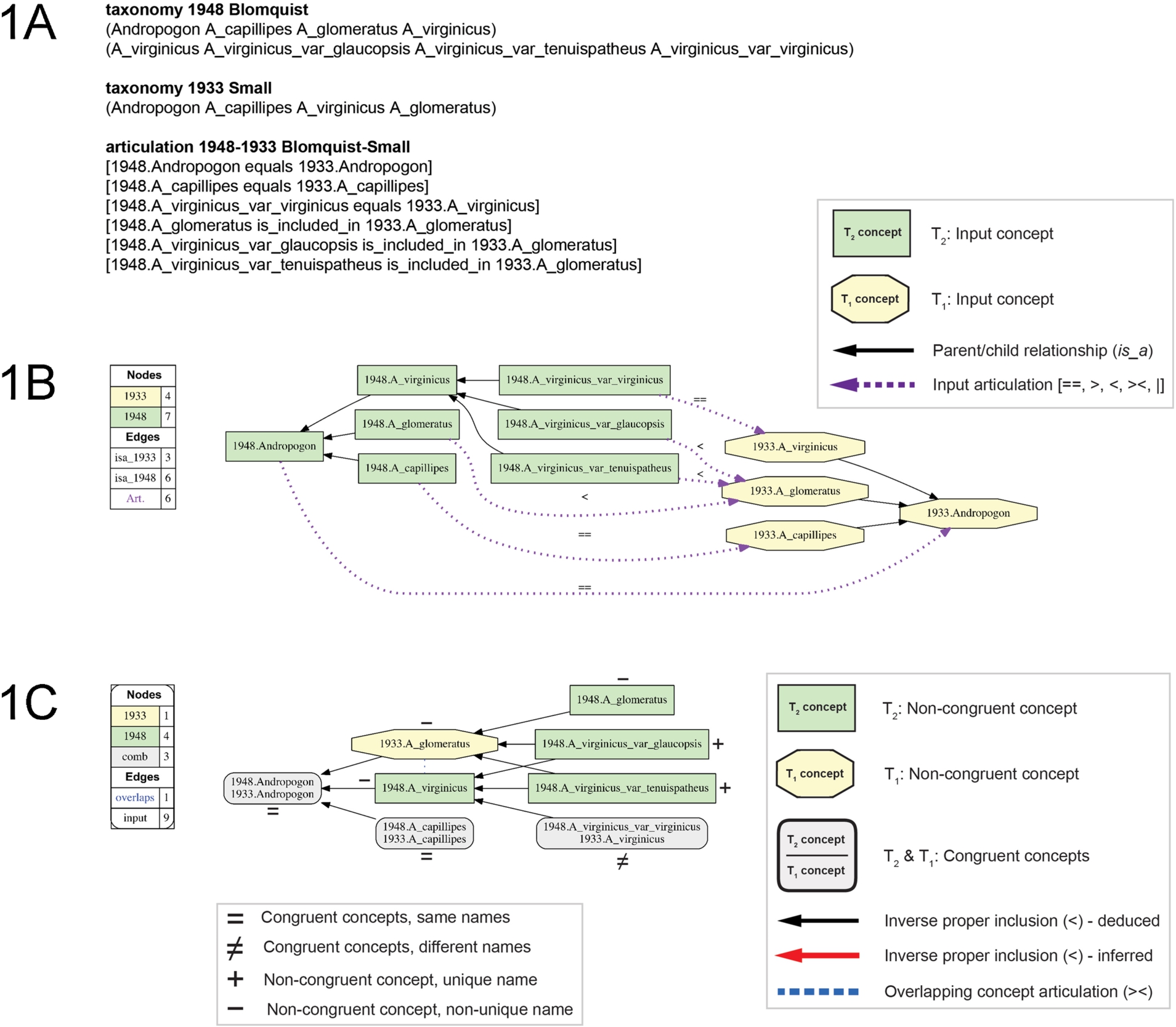
The set (C) of constraints applicable to taxonomy alignments are [87]: (1) non-emptiness – each concept has at least one representing instance; (2) sibling disjointness – children concepts of a parent concept are reciprocally disjoint, i.e., taxonomically exclusive of each other; and (3) parent coverage – parent concepts are completely circumscribed by (included in) the union of their children. For the present use case, all constraints apply by default, but in the toolkit each is relaxable where appropriate [14].
The toolkit functions with relevance to the Andro-UC are as follows (Fig. 1). (1) Visualization of each input taxonomy in the format of an is_a hierarchy, and including the set of user-provided articulations (Fig. 1B). (2) Analysis of logical consistency. If the input constraints are jointly inconsistent (constraint over-specification), then no alignments are obtained. (3) Inference and representation of one or more consistent alignments, grounded in the consistent user-provided articulations and additional, logically implied articulations. Alignments are generated in two data formats: (a) as the set of Maximally Informative Relations (MIR [84]) interpretable by humans and machines, and (b) as alignment visualizations that aid human comprehension of taxonomic in-/congruence across the input classifications and their constituent elements (Fig. 1C).
Fig. 2.
Tabular representation of the input alignment of taxonomic names and concepts used in the 11 succeeding classifications of the Andro-UC, as provided by Weakley [35,93,94]. Columns represent classifications whereas rows contain information on taxonomic name and concept identity (via taxonomic concept labels, see column headers). Cell shadings indicate congruent multi-concept lineages. Consecutive concept numbers (1–100) are reused in Fig. 3 for the purpose of comparison. See text for further details.
![Tabular representation of the input alignment of taxonomic names and concepts used in the 11 succeeding classifications of the Andro-UC, as provided by Weakley [35,93,94]. Columns represent classifications whereas rows contain information on taxonomic name and concept identity (via taxonomic concept labels, see column headers). Cell shadings indicate congruent multi-concept lineages. Consecutive concept numbers (1–100) are reused in Fig. 3 for the purpose of comparison. See text for further details.](https://content.iospress.com:443/media/sw/2016/7-6/sw-7-6-sw220/sw-7-sw220-g002.jpg)
Additional toolkit functions include logic-based diagnosis and repair options in the case of inconsistent input (=constraint over-specification), and visualizations of multiple alignments as aggregate and cluster views in the case of ambiguous input (=constraint under-specification) [15–17,23,61]. The latter visualizations can inform interactive decision tree routines, where the user is repeatedly prompted to resolve ambiguous (i.e., disjunctive) articulations, thereby reducing the number of possible word alignments. Both sets of functions are intended to aid the user in achieving consistent, well-specified alignments [33]. However, neither set of functions is needed to properly align the Andro-UC input, which by virtue of the unambiguously specified user input displayed in Fig. 2 already satisfies the criteria of consistency and sufficiency. We refer readers to other contributions where these issues are discussed in more detail [15,17,33,36,53].
4.Relationship of the RCC-5 multi-taxonomy alignment approach to other methods
To our knowledge, the specific combination of generating reasoner-inferred alignments between multiple biological taxonomies with RCC-5 articulations (and ASP reasoners) has no immediate precedent in the broader semantics domain. The logic foundations for this particular approach were developed in [16,43,86]. The step of modeling an input taxonomy as an is_a hierarchy is well established [37,66,89]. However, the remaining steps in our toolkit workflow diverge from existing ontology matching or provenance-tracking applications [18,21,24,52,80,89,92,97]. The use of RCC-5 articulations is the most significant difference, reflecting the preference of domain scientists for expressing concept relationships with these five basic set constraints [35,36,94].
Biodiversity scientists are often faced with use cases where sets of taxonomic occurrence records or entities can either be relevantly merged, or not, for information ingestion into subsequent analyses. This requirement, together with the notion that taxonomic boundaries are natural and empirically accessible [37], may motivate using RCC-5 over alternatives that express similarity ratios among individual concepts and concept hierarchies [92]. The latter are most appropriate for expressing “how semantically close?” two concepts are. However, for the biodiversity scientist this begs an additional question [34]: “are the differences significant, or negligible, for the purpose of merging data?” In this context, RCC-5 provides direct, actionable, set theory-based information for multi-taxonomy integration. The specific representation needs for biological taxonomies and derivations of FOL constraints are further discussed in [87].
Use of the RCC-5 articulations means that ambiguities due to incomplete knowledge in alignments are modeled through disjunctive articulations, which may be present in the input articulations, output MIR,33 or both [33]. Disjunctive articulations of the R32 lattice such as “
Parallel efforts to derive taxonomic concept alignments ‘directly’ from textual descriptions through the application of Natural Language Processing methods and phenotype ontologies are introduced in [22]. Other taxonomically focused integration projects that do not utilize RCC-5 include [10,13,66,73,88]. The degree to which the RCC-5 alignment approach is relevant to other field that model semantic drift requires further exploration.
5.Input and alignment conditions for the Andropogon use case
The Andro-UC has been selected to demonstrate the multi-taxonomy alignment approach for several reasons. First among these is the availability of preexisting concept circumscriptions and articulations through co-author Alan S. Weakley, an expert on the Flora (and floristic legacy) of the Southern and Mid-Atlantic States [93,94]. An earlier version of the use case was published in [35] and included eight classifications. Three recent classifications are herein added to the Andro-UC. The use case is furthermore suitable because it illustrates the considerable extent to which names and meanings may dissociate over time as Code-compliant names are applied to incongruent taxonomic classifications. The implications for integrating biodiversity data are thereby made clear. Moreover, with only 100 concepts, the Andro-UC is relatively small. Its outer taxonomic boundaries are well defined and stable throughout the 126-year time interval (1889–2015). These properties allow us to present the alignment visualizations within the confines of this contribution. Additional comments on the relevance of this use case and applicability of our approach to other alignment challenges are offered in the Discussion.
5.1.Taxonomic particulars
The history of the Andro-UC is reviewed in [35,93,94]. The 11 input classifications T1, …, T11 are each reproduced according to the source publications (Fig. 2). All input articulations were provided by the user in tabular format (Fig. 3), which readily facilitates translation into RCC-5 relations. Strictly speaking, the Andro-UC concerns the “A. virginicus-A. glomeratus complex” as circumscribed in [94]. The use case is thus much narrower in scope than the entire genus-level concept Andropogon sec. Clayton et al. (2013) [19], which includes more than 100 species-level concepts worldwide.
Fig. 3.
Hierarchical, multi-level representations of the 11 input classifications of the Andro-UC (see also Appendix A). Taxonomic name and concept identities (numbered from 1–100) as in Fig. 2.
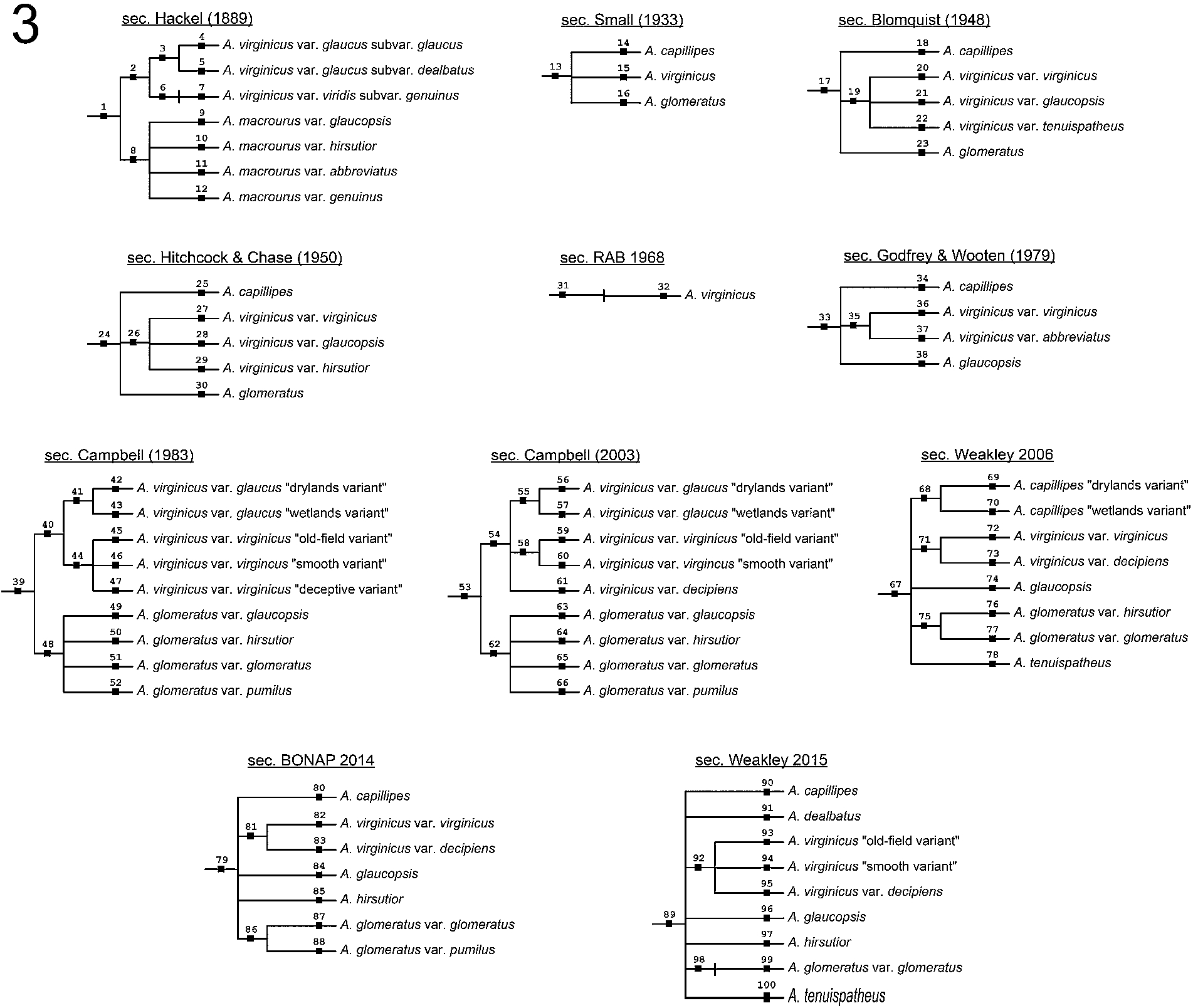
The classifications of the Andro-UC include, in chronological sequence (Figs 2 and 3): Hackel (1889) [49], Small (1933) [81], Blomquist (1948) [7], Hitchcock & Chase (1950) [50], Radford et al. (1968) [71], abbreviated as “RAB (1968)”, Godfrey & Wooten (1979) [45], Campbell (1983) [11], Campbell (2003) [12], Weakley (2006) [93], Kartesz (2014) [56], referred to as “BONAP (2014)”, and Weakley (2015) [94].
The tabular representation of Fig. 2 encodes taxonomic congruence as a function of occupying the same row (width). For instance, A. capillipes var. capillipes sec. Weakley (2015) (concept 90)
Another noteworthy aspect of the input representation are higher-ranked entities (compare Figs 2 and 3). These entities are not depicted in Fig. 2, because the table provided by Weakley emphasizes congruence among the narrowest concepts recognized in each classification. However, these higher-level entities are implied by conventions that guide the source taxonomies, and are usually made explicit therein. For instance, the acceptance of two variety-level concepts A. glomeratus var. hirsutior sec. Weakley (2006) (concept 76) and A. glomeratus var. glomeratus sec. Weakley (2006) (concept 77) (Fig. 2) implies recognition of the species-level concept A. glomeratus sec. Weakley (2006) (concept 75) (Fig. 3).
Our representations fully account for the implied higher-level taxonomic concepts, yielding comprehensive alignments with up to four levels (Fig. 3). Where necessary, we have added nominal (type) taxonomic names and concepts to represent comparable ranked entities at all levels; e.g., Andropogon virginicus var. viridis sec. Hackel (1889) was added (concept 6) and is comparable to Andropogon virginicus var. glaucus sec. Hackel (1889) (concept 3) of the same rank and source classification.
5.2.Input configuration, workflow execution, and reproducibility
The Euler/X toolkit is open source and available at [61]. The software can be cloned and then deployed on a desktop using the command-line interface. An overview of the toolkit’s reasoning and visualization options is available through the “help” command. Additional software dependencies include Python, the Answer Set Programming reasoners DLV [25] and Potassco (Gringo, claspD) [39], and GraphViz [38].
The input conventions for labeling concepts and representing parent/child (is_a) relationships and articulations are in accordance with [32–34,36]. They are exemplified in Fig. 1A for the 1948/1933 alignment. We limit our study to showing pairwise taxonomy alignments (see also Discussion), and therefore show outcomes for the following ten input configurations (Figs 4–6): 1933/1889 (Fig. 4A), 1948/1933 (Fig. 4B), 1950/1948 (Fig. 4C), 1968/1950 (Fig. 4D), 1979/1968 (Fig. 4E), 1983/1979 (Fig. 5B), 2003/1983 (Fig. 5C), 2006/2003 (Fig. 5D), 2014/2006 (Fig. 6A), and 2015/2014 (Fig. 6B). This strict chronological sequence is supplemented with two alignments; i.e., (1) 1979/1950 (Fig. 5A), which overcomes the gap in resolution generated by the intermediate, coarse RAB (1968) classification that contains only one species-level concept (Fig. 3); and (2) 2015/1889 (Fig. 6C), representing the largest possible time interval.
Fig. 4.
Visualizations for alignments 1–5 of the Andro-UC, 1889–1979. Representation conventions and annotations as in Fig. 1C. (A) Small (1933)/Hackel 1889 alignment; (B) Blomquist (1948)/Small (1933) alignment; (C) Hitchcock & Chase (1950)/Blomquist (1948) alignment; (D) RAB (1968)/Hitchcock & Chase (1950) alignment; (E) Godfrey & Wooten (1979)/RAB (1968).
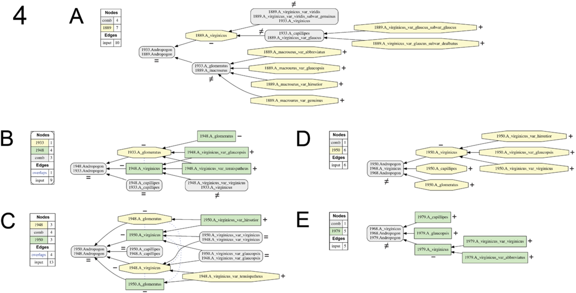
Fig. 5.
Visualizations for alignments 6–9 of the Andro-UC, 1950–2006. Representation conventions and annotations as in Fig. 1C. (A) Godfrey & Wooten (1979)/Hitchcock & Chase (1950); (B) Campbell (1983)/Godfrey & Wooten (1979); (C) Campbell (2003)/Campbell (1983); (D) Weakley (2006)/Campbell (2003).
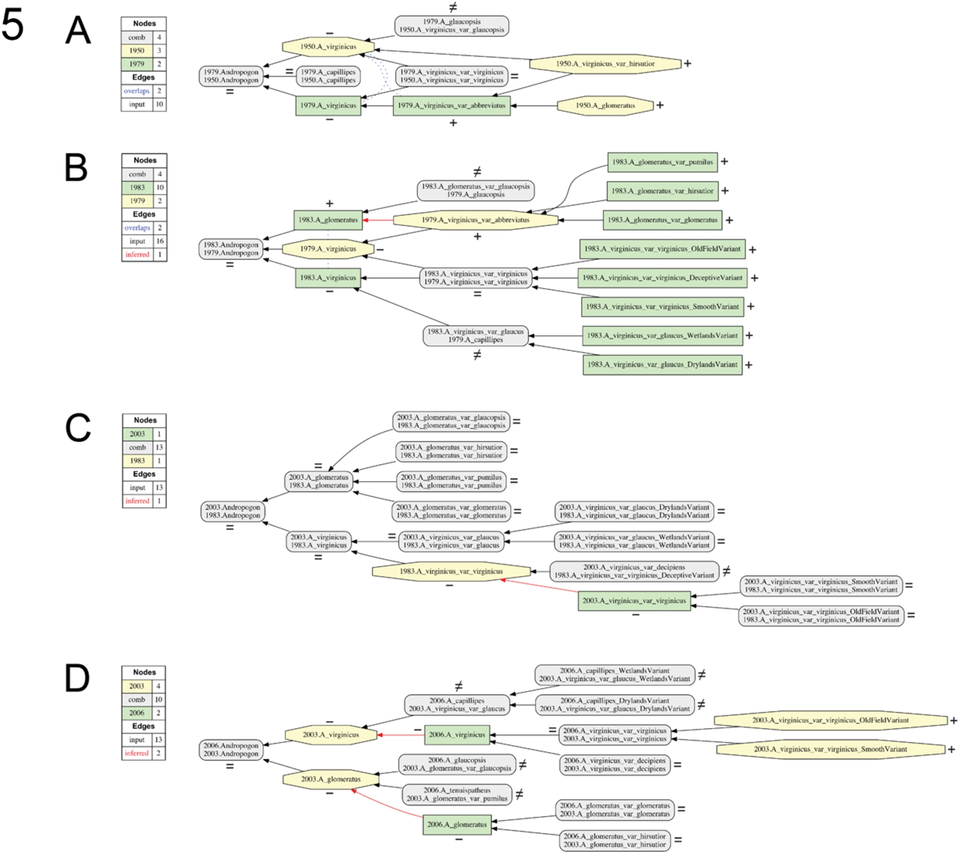
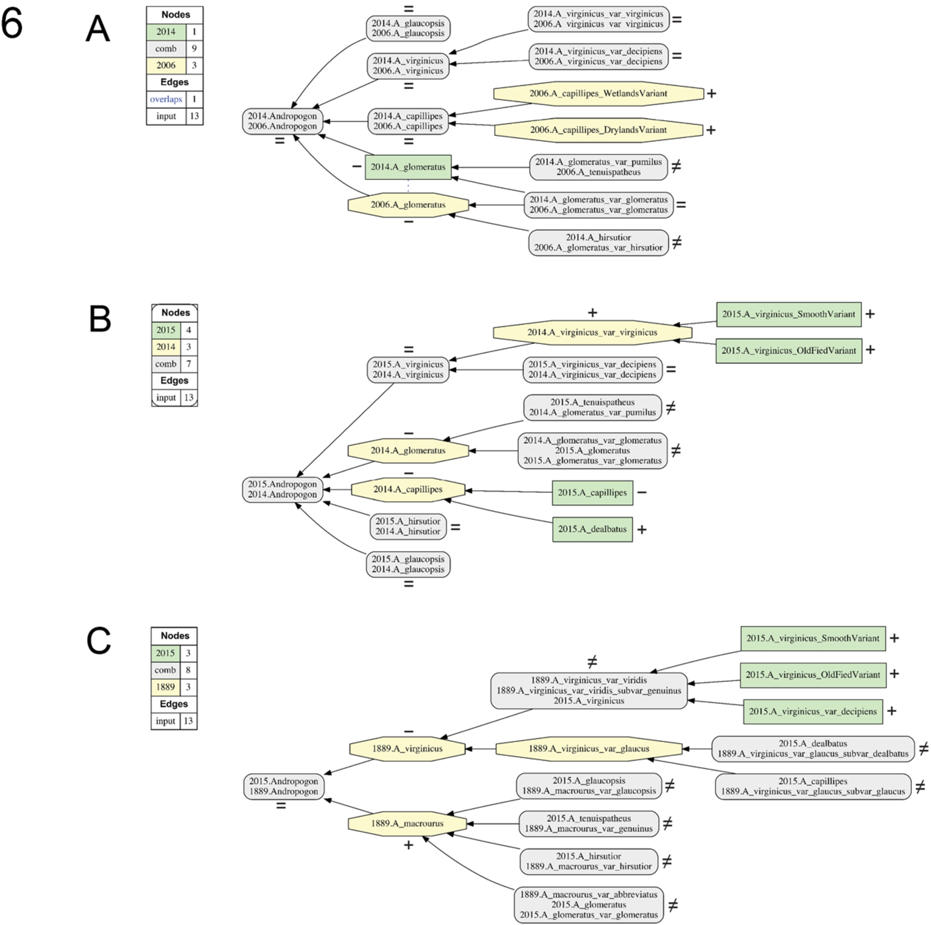
Fig. 6.
Visualizations for alignments 10–12 of the Andro-UC, 1889–2015. Representation conventions and annotations as in Fig. 1C. (A) BONAP (2014)/Weakley (2006); (B) Weakley (2015)/BONAP (2014); (C) Weakley (2015)/Hackel (1889).
In configuring the pairwise alignments, we represent the later (younger) taxonomy as T2 and the earlier (older) taxonomy as T1 [33]. Accordingly, the visualizations (Figs 1, 4–6) show concepts unique to T2 as green rectangles, and concepts unique to T1 as yellow octagons. Aligned regions with multiple congruent concepts are shown as grey rectangles with rounded corners (Fig. 1C). We use the shorthand of [36] for taxonomic concept labels, where (e.g.) Andropogon virginicus var. decipiens sec. Weakley (2015) becomes “2015.A_virginicus_var_decipiens”. The 12 input files (.txt format) for the Andro-UC are provided in Appendix A.
All alignments were obtained using “polynomial encoding/possible world/reduced containment graph” commands, which show overlapping articulations among input concepts as blue dashed lines in the output visualizations [14,16,61]. The commands generate the set of output MIR (.csv format) and GraphViz-rendered alignment visualizations (.pdf format).
The sets of Maximally Informative Relations (MIR) for each of the 12 alignments are provided in Appendix B. To ensure complete reproducibility, we have also prepared the Andro-UC use case as an experiment at http://recomputation.org/ [41,42].
6.Analyses of name:meaning dissociation
Quantitative analyses of evolving taxonomic name:meaning identity are central to this use case. To this end we provide three complementary groups of results [35,36,43]. First, we add annotations to the alignment regions (Figs 1C, 4–6), as follows. (1) For regions with multiple congruent concepts (
Table 1
Summary of taxonomic and nomenclatural identities of Euler regions across 12 alignment visualizations for the Andro-UC (see Figs 4–6). Columns show the number of aligned regions (excluding the congruent parent region), ratio of congruent (
| Alignment | T2/T1 | Figure | Regions1 | Reliable:Not | % Reliable | ||||
| 1 | 1933/1889 | 4A | 10 | 3:7 | 30.0% | 0:3 | 6:1 | 6:4 | 60.0% |
| 2 | 1948/1933 | 4B | 7 | 2:5 | 28.6% | 1:1 | 2:3 | 3:4 | 42.9% |
| 3 | 1950/1948 | 4C | 9 | 3:6 | 33.3% | 3:0 | 2:4 | 5:4 | 55.6% |
| 4 | 1968/1950 | 4D | 6 | 0:6 | 0.0% | 0:0 | 5:1 | 5:1 | 83.3% |
| 5 | 1979/1968 | 4E | 5 | 0:5 | 0.0% | 0:0 | 4:1 | 4:1 | 80.0% |
| 6 | 1979/1950 | 5A | 8 | 3:5 | 37.5% | 2:1 | 3:2 | 5:3 | 62.5% |
| 7 | 1983/1979 | 5B | 15 | 3:12 | 20.0% | 1:2 | 10:2 | 11:4 | 73.3% |
| 8 | 2003/1983 | 5C | 14 | 12:2 | 85.7% | 11:1 | 0:2 | 11:3 | 78.6% |
| 9 | 2006/2003 | 5D | 15 | 9:6 | 60.0% | 4:5 | 2:4 | 6:9 | 40.0% |
| 10 | 2014/2006 | 6A | 12 | 8:4 | 66.7% | 6:2 | 2:2 | 8:4 | 66.7% |
| 11 | 2015/2014 | 6B | 13 | 6:7 | 46.2% | 4:2 | 4:3 | 8:5 | 61.5% |
| 12 | 2015/1889 | 6C | 13 | 7:6 | 53.8% | 0:7 | 5:1 | 5:8 | 38.5% |
| Totals | − | − | 127 | 56:71 | 44.1% | 32:24 | 45:26 | 77:50 | 60.6% |
1 Number of aligned regions excludes the root/parent region (“Andropogon” sec. auctorum) whose name is held constant throughout
Second, we compute simple name:meaning identity analyses based on the output MIR data (Tables 2 and 3). For each alignment, we record the numbers of input concepts (T2, T1), input articulations (A), and MIR. The latter are partitioned according to each RCC-5 articulation (Table 2). As above, MIR articulating root concepts are excluded. The quotient of (1) the number of congruent articulations (
Table 2
Summary of numbers of input concepts (T2/T1) and input articulations (A) for the 12 alignments of the Andro-UC, and of the Maximally Informative Relations (MIR), including totals and partitions according to each type of RCC-5 articulation. Legend: Rel.
| Alignment | Concepts T2 | Concepts T1 | Articulations | MIR1 | > | < | | | Rel. | ||
| 1 | 4 | 12 | 8 | 33 (48) | 4 | 6 | 2 | 0 | 21 | 100% |
| 2 | 7 | 4 | 6 | 18 (28) | 2 | 1 | 3 | 1 | 11 | 50.0% |
| 3 | 7 | 7 | 7 | 36 (49) | 3 | 3 | 3 | 4 | 23 | 42.9% |
| 4 | 2 | 7 | 1 | 6 (14) | 0 | 6 | 0 | 0 | 0 | 0.0% |
| 5 | 7 | 2 | 1 | 5 (12) | 0 | 0 | 5 | 0 | 0 | 0.0% |
| 6 | 6 | 7 | 6 | 30 (42) | 3 | 5 | 2 | 2 | 18 | 50.0% |
| 7 | 14 | 6 | 10 | 65 (84) | 3 | 4 | 15 | 2 | 41 | 50.0% |
| 8 | 14 | 14 | 10 | 169 (196) | 12 | 15 | 17 | 0 | 125 | 85.7% |
| 9 | 12 | 14 | 10 | 143 (168) | 9 | 10 | 13 | 0 | 111 | 75.0% |
| 10 | 10 | 12 | 9 | 99 (120) | 8 | 6 | 4 | 1 | 80 | 80.0% |
| 11 | 12 | 10 | 10 | 99 (120) | 7 | 2 | 10 | 0 | 80 | 70.0% |
| 12 | 12 | 12 | 10 | 121 (144) | 9 | 0 | 19 | 0 | 93 | 75.0% |
| Totals | 106 | 107 | 88 | 824 (1025) | 60 | 58 | 93 | 10 | 603 | 56.6% |
1 Number in parentheses includes all MIR that articulate the root/parent region (“Andropogon” sec. auctorum) which are otherwise excluded from the counts
Table 3
Analysis of taxonomic name:meaning relationships in the 12 alignments of the Andro-UC, based on the 824 Maximally Informative Relations (MIR), and including assessments of reliable names [R] and unreliable names [UR]. Legend:
| Alignment | Total R | Total UR | ||||||||||
| 1 | 0 | 4 | 0 | 6 | 1 | 1 | 0 | 0 | 0 | 21 | 28 | 5 |
| 2 | 1 | 1 | 1 | 0 | 1 | 2 | 0 | 1 | 0 | 11 | 15 | 3 |
| 3 | 3 | 0 | 0 | 3 | 0 | 3 | 2 | 2 | 0 | 23 | 34 | 2 |
| 4 | 0 | 0 | 1 | 5 | 0 | 0 | 0 | 0 | 0 | 0 | 5 | 1 |
| 5 | 0 | 0 | 0 | 0 | 1 | 4 | 0 | 0 | 0 | 0 | 4 | 1 |
| 6 | 2 | 1 | 0 | 5 | 0 | 2 | 1 | 1 | 0 | 18 | 28 | 2 |
| 7 | 1 | 2 | 0 | 4 | 0 | 15 | 1 | 1 | 0 | 41 | 62 | 3 |
| 8 | 11 | 1 | 0 | 15 | 1 | 16 | 0 | 0 | 0 | 125 | 167 | 2 |
| 9 | 4 | 5 | 0 | 10 | 2 | 11 | 0 | 0 | 0 | 111 | 136 | 7 |
| 10 | 6 | 2 | 0 | 6 | 0 | 4 | 1 | 0 | 0 | 80 | 96 | 3 |
| 11 | 5 | 2 | 0 | 2 | 2 | 8 | 0 | 0 | 0 | 80 | 95 | 4 |
| 12 | 0 | 9 | 0 | 0 | 1 | 18 | 0 | 0 | 0 | 93 | 111 | 10 |
| Totals | 33 | 27 | 2 | 56 | 9 | 84 | 5 | 5 | 0 | 603 | 781 | 43 |
Third, we reinterpret the input displayed in Fig. 2 to evaluate the performance of names as concept identifiers over the entire 1889–2015 interval. We adopt Remsen’s [74] notion of cardinality to address two questions. First, how many usages and meanings are associated with each of the 36 unique taxonomic names in the Andro-UC (Table 4)? For instance, a name:meaning cardinality of 1:3 indicates that an identical name was used in (at least) three classifications, and associated with three reciprocally incongruent taxonomic meanings. Second, how many (non-identical) names are associated with each of the 21 congruent sets (or lineages) of taxonomic meanings in the Andro-UC (Table 5)? For instance, a name:meaning cardinality of 3:1 indicates that three non-identical names were used to identify meanings (or meaning chains [59]) across classifications that are taxonomically congruent. For the purpose of labeling the chains, we select the most recent (youngest) taxonomic concept label that anchors an instance of the chain, which extends to congruent concepts in one or more preceding classifications. An example is 2014.A_capillipes (youngest concept label, used to label the chain)
In addition to showing the dynamics of name:meaning cardinality, Tables 4 and 5 indicate how often certain names or meanings re-/appear in the Andro-UC, and whether their occurrences are continuous or interrupted by intermediate classifications.
Table 4
Analysis of name:meaning cardinality for the entire Andro-UC, based on 88 name usages of 36 taxonomic names corresponding to 46 unique (sets of) taxonomic meanings. Cell values indicate (1) that the name is used and (2) which of the 1–n meanings is symbolized by the name in the corresponding classification. Names are ordered according to their frequency of use in the 12 classifications. Non-congruent (sets of) meanings associated with each name are numbered in reverse chronological order, i.e., starting with the 2015 taxonomy. See also Fig. 1
| # | Taxonomic name | 1889 | 1933 | 1948 | 1950 | 1968 | 1979 | 1983 | 2003 | 2006 | 2014 | 2015 | Usages | Meanings |
| 1 | A. virginicus | 2 | 1 | 6 | 5 | 4 | 3 | 2 | 2 | 1 | 1 | 1 | 11 | 6 |
| 2 | A. glomeratus | 4 | 3 | 2 | 4 | 4 | 3 | 2 | 1 | 8 | 4 | |||
| 3 | A. capillipes | 2 | 2 | 2 | 2 | 2 | 2 | 1 | 7 | 2 | ||||
| 4 | A. virginicus var. virginicus | 2 | 2 | 2 | 2 | 1 | 1 | 1 | 6 | 2 | ||||
| 5 | A. glomeratus var. glomeratus | 1 | 1 | 1 | 1 | 1 | 5 | 1 | ||||||
| 6 | A. glaucopsis | 1 | 1 | 1 | 1 | 4 | 1 | |||||||
| 7 | A. virginicus var. decipiens | 1 | 1 | 1 | 1 | 4 | 1 | |||||||
| 8 | A. glomeratus var. hirsutior | 1 | 1 | 1 | 3 | 1 | ||||||||
| 9 | A. glomeratus var. pumilus | 1 | 1 | 1 | 3 | 1 | ||||||||
| 10 | A. virginicus var. glaucus | 1 | 1 | 1 | 3 | 1 | ||||||||
| 11 | A. glomeratus var. glaucopsis | 1 | 1 | 2 | 1 | |||||||||
| 12 | A. hirsutior | 1 | 1 | 2 | 1 | |||||||||
| 13 | A. tenuispatheus | 1 | 1 | 2 | 1 | |||||||||
| 14 | A. virginicus var. glaucopsis | 1 | 1 | 2 | 1 | |||||||||
| 15 | A. virginicus var. glaucus “drylands variant” | 1 | 1 | 2 | 1 | |||||||||
| 16 | A. virginicus var. glaucus “wetlands variant” | 1 | 1 | 2 | 1 | |||||||||
| 17 | A. virginicus var. virginicus “old-field variant” | 1 | 1 | 2 | 1 | |||||||||
| 18 | A. virginicus var. virginicus “smooth variant” | 1 | 1 | 2 | 1 | |||||||||
| 19 | A. capillipes “drylands variant” | 1 | 1 | 1 | ||||||||||
| 20 | A. capillipes “wetlands variant” | 1 | 1 | 1 | ||||||||||
| 21 | A. dealbatus | 1 | 1 | 1 | ||||||||||
| 22 | A. macrourus | 1 | 1 | 1 | ||||||||||
| 23 | A. macrourus var. abbreviatus | 1 | 1 | 1 | ||||||||||
| 24 | A. macrourus var. genuinus | 1 | 1 | 1 | ||||||||||
| 25 | A. macrourus var. glaucopsis | 1 | 1 | 1 | ||||||||||
| 26 | A. macrourus var. hirsutior | 1 | 1 | 1 | ||||||||||
| 27 | A. virginicus “old-field variant” | 1 | 1 | 1 | ||||||||||
| 28 | A. virginicus “smooth variant” | 1 | 1 | 1 | ||||||||||
| 29 | A. virginicus var. abbreviatus | 1 | 1 | 1 | ||||||||||
| 30 | A. virginicus var. glaucus subvar. dealbatus | 1 | 1 | 1 | ||||||||||
| 31 | A. virginicus var. glaucus subvar. glaucus | 1 | 1 | 1 | ||||||||||
| 32 | A. virginicus var. hirsutior | 1 | 1 | 1 | ||||||||||
| 33 | A. virginicus var. tenuispatheus | 1 | 1 | 1 | ||||||||||
| 34 | A. virginicus var. virginicus “deceptive variant” | 1 | 1 | 1 | ||||||||||
| 35 | A. virginicus var. viridis | 1 | 1 | 1 | ||||||||||
| 36 | A. virginicus var. viridis subvar. genuinus | 1 | 1 | 1 | ||||||||||
| Concepts per taxonomy/Cumulative totals | 11 | 3 | 6 | 6 | 1 | 5 | 13 | 13 | 11 | 9 | 11 | 88 | 46 | |
Table 5
Analysis of taxonomic name:meaning cardinality for the entire Andro-UC, based on 85 occurrences of concepts (“members”) that participate in 21 congruent concept chains, where individual chains are labeled with 1–4 taxonomic names. Cell values indicate (1) that the concept is an element of the chain and (2) which of the 1–n names is used to symbolize the member in the corresponding classification. Each of the 21 chains is labeled by its most recent member, and concept lineages are ordered accordingly. Non-identical (sets of) names associated with each chain are numbered in reverse chronological order, i.e., starting with their name in the 2015 taxonomy. See also Fig. 1 and Table 4
| # | Concept chain label | 1889 | 1933 | 1948 | 1950 | 1968 | 1979 | 1983 | 2003 | 2006 | 2014 | 2015 | Members | Names |
| 1 | 2015.A_capillipes | 4 | 3 | 3 | 2 | 1 | 5 | 4 | ||||||
| 2 | 2015.A_dealbatus | 4 | 3 | 3 | 2 | 1 | 5 | 4 | ||||||
| 3 | 2015.A_virginicus | 3(4) | 1 | 2 | 2 | 2 | 2 | 1 | 1 | 1 | 8 | 3(4) | ||
| 4 | 2015.A_virginicus_OldFieldVariant | 2 | 2 | 1 | 3 | 2 | ||||||||
| 5 | 2015.A_virginicus_SmoothVariant | 2 | 2 | 1 | 3 | 2 | ||||||||
| 6 | 2015.A_virginicus_var_decipiens | 2 | 1 | 1 | 1 | 1 | 5 | 2 | ||||||
| 7 | 2015.A_glaucopsis | 4 | 3 | 3 | 1 | 2 | 2 | 1 | 1 | 1 | 9 | 4 | ||
| 8 | 2015.A_hirsutior | 4 | 3 | 2 | 2 | 2 | 1 | 1 | 7 | 4 | ||||
| 9 | 2015.A_glomeratus_var_glomeratus | 2 | 1 | 1 | 1 | 1 | 1(2) | 6 | 2(3) | |||||
| 10 | 2015.A_tenuispatheus | 4 | 3 | 2 | 2 | 1 | 2 | 1 | 7 | 4 | ||||
| 11 | 2014.A_capillipes | 2 | 1 | 1 | 1 | 1 | 2 | 2 | 1 | 1 | 8 | 2 | ||
| 12 | 2014.A_virginicus_var_virginicus | 1 | 1 | 1 | 3 | 1 | ||||||||
| 13 | 2014.A_glomeratus | 1 | 1 | 2 | 1 | |||||||||
| 14 | 2006.A_glomeratus | 1 | 1 | 2 | 1 | |||||||||
| 15 | 2003.A_virginicus | 1 | 1 | 1 | 3 | 1 | ||||||||
| 16 | 2003.A_glomeratus | 2 | 1 | 1 | 1 | 4 | 2 | |||||||
| 17 | 1979.A_virginicus | 1 | 1 | 1 | ||||||||||
| 18 | 1979.A_virginicus_var_abbreviatus | 1 | 1 | 1 | ||||||||||
| 19 | 1968.A_virginicus | 1 | 1 | 1 | ||||||||||
| 20 | 1950.A_virginicus | 1 | 1 | 1 | ||||||||||
| 21 | 1948.A_virginicus | 1 | 1 | 1 | ||||||||||
| Concepts per taxonomy/Cumulative totals | 11 | 3 | 6 | 6 | 1 | 5 | 13 | 13 | 11 | 9 | 11 | 85 | 44(46) | |
7.Results
7.1.Extent and origins of taxonomic incongruence
Each of the 12 input configurations yields a single, consistent, and unambiguously resolved alignment (Figs 4–6). The 12 visualizations clearly illustrate that none of the paired input taxonomies are entirely congruent, instead showing 2–12 unique regions (compare Figs 5B and 5C), and an overall ratio of 56 congruent to 71 non-congruent regions (Table 1). While we cannot examine each alignment in fine detail, we highlight select phenomena that capture the extent and causes of taxonomic incongruence in the Andro-UC. One cause for incongruence is unequal granularity across classifications. For instance, at the lowest taxonomic level, classifications authored from 1933 to 1979 recognize 1–5 concepts, whereas taxonomies published outside of this interval accept 7–9 concepts (Figs 2 and 3). Such differences cause the more finely resolving taxonomy to have one or more non-congruent (properly included) low-level concepts in comparison to its counterpart (e.g., Figs 4A and 5B). For instance, alignments of any taxonomy to that of the most coarse-grained RAB (1968) classification are only congruent with regards to the root-level concepts (Figs 4D and 4E), given that RAB (1968) recognize no additional taxonomic subdivisions within the complex. In the context of its immediate predecessor and successor (Figs 2, 4D, 4E, and 5A), the 1968 classification appears disruptive because the chain of taxonomic resolution between Hitchcock & Chase (1950) and Godfrey & Wooten (1979) is not propagated in RAB (1968).
Taxonomies produced in 1983 or later show higher levels of congruence between their finest-degree entities (Figs 5C, 5D, and 6). By and large, taxonomists publishing in the past 30 years have adopted Campbell’s (1983) perspective on how finely one should differentiate units within the complex. Incongruences among these recent perspectives are rooted mainly in disagreements on how to name and integrate low-level entities into parent concepts. Interestingly, Hackel (1889) already recognized seven low-level entities, and in that sense his classification is more congruent with contemporary perspectives (Fig. 6C) than with those published in 1933–1979.
In addition to unequal granularity, five alignments show overlapping (
The 1950/1948 alignment represents an interesting case of overlap (Fig. 4C). Both Hitchcock & Chase (1950) and Blomquist (1948) recognize three identically named species-level concepts within in the complex, one of which is also taxonomically congruent (1950.A_capillipes
Of particular note is the articulation 1950.A_glomeratus
Generalizing the phenomenon exemplified in the 1950/1948 alignment, we observe that overlap of two (or more) concepts creates combined concept regions for which there are no unique names in the respective input taxonomies. Nevertheless, identifiers for these alignment regions are required to express the extent to which the input concepts can be aligned with each other. The toolkit’s “combined concepts” command uniquely labels these regions (see [33]).
Overall, occurrences of differential resolution and overlapping concepts in the Andro-UC result in pairwise alignments with 5–15 regions (Table 1). Taking the 12 alignments in conjunction, 44.1% of the 127 inferred alignment regions are taxonomically congruent (range: 0.0–85.7%), leaving the remaining 55.9% incongruent. This ratio of in-/congruence between paired taxonomies is the semantic basis of the dis-/agreements that taxonomic names are suited to identify and track, though only up to a point, as we analyze in the next section.
7.2.Quantification of name:meaning dissociation
Taxonomic names are reliable identifiers of taxonomic in-/congruence for 77/127 (60.6%) of the regions present in the 12 pairwise alignments of the Andro-UC (range: 38.5–83.3%) (Table 1). The highest ratios are obtained for the 1968/1950 and 1979/1968 alignments. The latter include no congruent regions, since every unique name also symbolizes a unique alignment region (Figs 4D and 4E). The 5:13 ratio (38.5%) for the 2015/1889 alignment (Fig. 6C) is low as expected. In particular, 0/7 congruent concept regions in this 126 year-spanning alignment have reliable names; i.e., each of these regions is labeled by two non-identical names. However, taxonomic names in the Andro-UC do not necessarily perform better over short time intervals, or in alignments whose input taxonomies are closer to the present (2015). One example is the 2006/2003 alignment (Fig. 5D), which has an undesirable 6:9 ratio (40.0%) of reliable:unreliable names.
The 824 output MIR permit finer assessments of name:meaning dissociation (Table 3). Accordingly, among all 60 instances of pairwise taxonomic concept congruence (
Among the remaining 161 non-congruent articulations (>, <,
Quantification of name:meaning cardinality over the 126-year period of the Andro-UC reveals that 18/36 taxonomic names (50.0%) have been used in multiple treatments, whereas the other 18 names are particular to single treatments (Table 4). Cumulatively, the use case entails 88 taxonomic name usages and 46 unique name:meaning combinations (ratio: 1.91:1). Only one name – A. virginicus – is used in every classification. Three additional names – i.e., A. capillipes, A. glomeratus, and A. virginicus var. virginicus – are used in 6–8 of the 11 input classifications. The other (32/36) names occur in less than half of them. Most, though not all, taxonomic names with 2–4 usages appear in temporally consecutive taxonomies (relation: 9/13).
The most frequently used name – A. virginicus – also has the highest number of incongruent taxonomic meanings, with a name:meaning cardinality of 1:6 (Table 4). Six consecutive classifications authored in 1933–1983 all propagate incongruent meanings of “A. virginicus” (Fig. 2). Only three additional names have more than one meaning in the Andro-UC; viz. A. capillipes (name:meaning cardinality = 1:2), A. glomeratus (1:4) and A. virginicus var. virginicus (1:2).
The 88 name usages in the Andro-UC correspond to 21 chains of taxonomically congruent concepts (Table 5). Of these, the chain symbolized by 2015.A_glaucopsis (most recent member) is the longest, with elements appearing in 9/11 classifications and under four non-identical names. Other long chains include 2015.A_virginicus (8 usages/4 non-identical names), 2014.A_capillipes (8/2), 2015.A_hirsutior (7/4), and 2015.A_tenuispatheus (7/4). At the other end of the spectrum, five concepts display globally unique meanings that whose meanings are unique to one classification (two authored in 1979; and one in 1968, 1950, and 1948, respectively).
At the other end of the length spectrum, there are five concepts whose meanings are unique to one classification (two authored in 1979; and one in 1968, 1950, and 1948, respectively).
The least favorable name:meaning cardinality among the 21 chains 4:1; meaning that four non-identical names are used to identify sets of taxonomically congruent concepts. This ratio applies to six concept chains: 2015.A_capillipes, 2015.A_dealbatus, 2015.A_virginicus, 2015.A_glaucopsis, 2015.A_hirsutior, and 2015.A_tenuispatheus. Conversely, a cardinality of 1:1 is obtained in 9/21 chains, of which only four have more than one usage (Table 5).
The information shown in Tables 4 and 5 provides an intuitive sense of how taxonomic names fare in the longer term as identifiers of taxonomy meanings in the Andro-UC. The performance of names should be evaluated in the context of taxonomic stability. High taxonomic stability would be reflected in an abundance of occupied cells in Table 5, because early-authored concepts would have congruent successors – with either identical or non-identical names – in the 1889–2015 time interval. This is not the case: only 85/231 cells (36.8%) have values, and 14/16 chains (87.5%) with multiple elements are ‘interrupted’.
In spite of persistent taxonomic meaning evolution, identifiers could nevertheless (in principle) be designed to achieve a name:meaning cardinality of 1:1. In that case taxonomic names would simultaneously show a score of 1 in the “Meanings” column of Table 4 and a score of 1 in the “Names” column of Table 5. Thirty-two names meet the former condition, and nine names meet the latter condition. However, the intersection of these two sets of includes only one name – A. virginicus var. abbreviatus. This name, used exclusively in Godfrey & Wooten (1979), is the only identifier that requires neither the “sec.” annotation nor an articulation with RCC-5 to reliably identify its associated meaning in the entire Andro-UC. The remaining 35/36 names are syntactically and/or semantically ‘compromised’, showing name:meaning cardinality relations other than 1:1. This outcome is also reflected in the accumulation of numbers greater than 1 across the columns of Tables 4 and 5.
In summary, even though names used in the Andro-UC act as identifiers of meanings with reliability ratios of 56.6% or higher in the local, pairwise alignments (Tables 1–3), their global reliability is such that >97.2% diverge from an ideal name:meaning cardinality of 1:1. This assessment remains adequate even if taxonomic change is taken into account.
8.Discussion
We focus our discussion on the performance of names as identifiers of taxonomic concepts, emphasizing on new insights gained from our representation and reasoning approach. We also assess the relevance of the RCC-5 multi-taxonomy alignment approach for wider application (with scalability implications) in the biodiversity data realm, and potential applications to other semantic integration tasks.
8.1.New knowledge products
What aspects of our approach are new and valuable? The Andro-UC illustrates the unique ability of RCC-5 multi-taxonomic alignments to resolve taxonomic meaning evolution at more granular levels than is possible using taxonomic names and nomenclatural relationships [70]. This follows directly from the input information – we can only represent and align the entities shown in Fig. 1 if taxonomic concept labels and RCC-5 articulations are used. Critically, the approach requires an initial set of articulations provided by human (expert) users, and grounded in their assessments of pertinent taxonomic evidence, that satisfy criteria of consistency and (lack of) ambiguity to yield well-specified alignments. Compliance with these criteria is achieved by the interactive toolkit workflow [33].
New knowledge products for the Andro-UC include the output MIR, alignment visualizations, and name:meaning cardinality analyses. Through the reasoning process, the set of 88 user-provided input articulations is logically tested and augmented to yield 824 Maximally Informative Relations (1025 MIR if the root concepts are included). The MIR derived for each alignment can be queried to determine whether any concept pairs (and ancillary biological data) are suitable for integration, or not [36,43,53,85,86]. In particular, articulations of congruence (“yes, integrate”) and exclusion (“no”) between two concepts are reciprocally actionable in this context. Proper inclusion and inverse proper inclusion are least unilaterally actionable without ambiguity (“add data assigned to the less inclusive concept to those of the more inclusive one”). Overlap is the most challenging articulation for the purpose of merging ancillary information. However, in some instances overlap at higher levels in an alignment can be resolved into proper inclusion at lower levels. For instance, the 2014/2006 alignment (Fig. 6A) shows the articulation 2014.A_glomeratus
The alignment visualizations are logically congruent with the output MIR [14,16,23,87]. Their unique value lies in aiding human users to understand multi-concept relationships through tree-like representations. Visualization tools for multi-taxonomy relationships have advanced significantly over the past 20 years [3,5,16,46,47,98]. Nevertheless, the Euler/X toolkit is the first platform to leverage RCC-5 relationships and logic reasoning to yield comprehensive, tree-like alignment visualizations.
The visualizations communicate uniquely valuable information. For instance, Figs 1–3 all show information related to the 1948/1933 alignment. Figure 2 effectively visualizes the lowest-level entities and articulations of the entire Andro-UC, but is not well suited for input taxonomies nested into three or more ranks (or phylogenetic levels). Such tables are ‘flattened’ into two dimensions. Figure 3, in turn, can shows all nested entities for the individual 1948/1933 taxonomies, but does not provide accurate multi-concept alignment information. Using names to navigate across these trees may lead to erroneous conclusions such as 1948.A_virginicus | 1933.A_glomeratus, when the proper articulation is
In contrast, the alignment visualizations (Fig. 1) simultaneously communicate information about nomenclatural identity, multi-level tree hierarchy, and multi-tree in-/congruence. Their interpretation is intuitive; for instance, the proportion and position of grey squares versus green rectangles or yellow octagons communicate the extent and localization of taxonomic in-/congruence in an alignment (compare, e.g., Figs 5B and 5C). The relative occurrences of (=, ≠, +, −) annotations show the degree to which taxonomic names can reliably integrate taxonomic meanings.
8.2.Building better identifiers for biodiversity data
How relevant is our representation approach to the broader, semantics-facilitated biodiversity data realm? Multiple reviewers raised this important question. We think that it is too early to attempt a comprehensive answer. Technical, scientific, cognitive-evolutionary, and socio-cultural constraints affect how identifier granularity is managed in the biological domain. Predicting how the RCC-5 alignment approach will fare in light of these trade-offs is beyond the scope of this analysis. We can, however, assess the particulars and generalities of the Andro-UC, and what it teaches us about identifying and linking taxonomically identified information in open-ended biodiversity data environments.
The scale of the Andro-UC is small. Weakley’s (2015) classification recognizes seven species-level concepts – more than any other taxonomy. The taxonomic history is evidently complex, but no more complicated than that of many other continuously revised groups [1,20,32,35,43,68,77,90]. The poor performance of names as identifiers of divergent taxonomic meanings is not exceptional for the field (herein broadly defined to include phylogenetics).
The problem of name:meaning dissociation in biological taxonomy is systemic. It is rooted in Code-mandated principles that promote stability and change in naming (largely) as a function of nomenclatural type identity and priority. To some degree the inadequacies are manageable through social processes, including conservative re-/naming practices or ‘standardized’ taxonomies [6,44,55,79,91]. In practice, the long-term drawbacks of using taxonomic names as concept identifiers are frequently mitigated by the ability of well-trained human scientists to contextualize name usages and thereby infer the intended meanings [30,32,69]. However, no counteracting human practice can alter the insight that taxonomic names and nomenclatural relationships are fundamentally not designed to track granular similarities and differences in taxonomic meaning of the sort exemplified in the Andro-UC. Computer algorithms in particular struggle with inferring what “Andropogon virginicus” means ‘in the currently intended context’ [62], i.e., when the relevant context of the name usage is not made explicit. Something beyond the type-anchored name identity is needed if taxonomic perspectives are to be translated into entities fit for use in open-ended, semantics-enabled information environments.
Specifying the referential extension of taxonomic names for reliable reuse requires more than ostension (the act of pointing) to exemplars (types). Ostensive definitions of taxonomic meanings are bound to under-specify the intended meanings in many applied contexts, such as those of the Andro-UC. Instead it is more appropriate to model the name-to-(currently-perceived-)taxon linkage as a matter of theory construction [31,75]. The challenge of integrating biodiversity data then becomes one of aligning multiple taxonomic theories, which can be modeled with the RCC-5 approach.
The aforementioned insufficiencies are most apparent in cases of multi-concept overlap. Such cases are frequent in taxonomy, and they cannot be reduced to the differences in degree of resolution [26,65,68,77]. As an example, the 1950/1948 classifications of the Andro-UC concur that there are three identically named species-level concepts entailed in the complex (Fig. 4C). They also concur that 1950/1948.A_virginicus has three variety-level child concepts. However, they disagree on the extent to which the available, type-anchored names reach out to perceived, and necessarily more inclusive, taxa presumed (more precisely: theorized) to constitute natural, evolutionary entities [9]. As a consequence of this differential inference of ‘extra-typical’ taxonomic boundaries, the four 1950/1948 species-level concepts overlap in complex ways (Fig. 4C). Such multi-theory overlap is more frequent at higher taxonomic levels, where the performance of names as identifiers of taxonomic meanings becomes increasingly poor [33,35,36].
The herein demonstrated alignment approach paves the way for building better taxonomic concept identifiers and multi-taxonomy resolution services.
8.3.Scalability of the RCC-5 alignment approach
How widely applicable (or scalable) is the RCC-5 multi-taxonomy alignment approach within the field of biological taxonomy? Generally speaking, reasoning about taxonomies with RCC-5 remains in its infancy [16,33,36,43,87]. At present, the Euler/X toolkit can effectively process consistent, well-specified, pairwise input taxonomies with up to 200–400 concepts each [14,16,61]. While this scale is sufficient for small- to medium-sized alignment use cases, future toolkit development should concentrate on modularizing the reasoning process, specifically by using a divide-and-conquer approach that better leverages the hierarchical structure of the input constraints and dynamic user/reasoner interactions. Demonstrating the practical value of the approach requires making the toolkit accessible to larger use cases and biodiversity data environment where taxonomy evolution is an important variable to identify and control.
The analysis of the Andro-UC demonstrates the potential of reasoning about taxonomies and at the same time leaves much room for further work. In particular, the 11 input classifications allow for 55 pairwise comparisons, of which only 12 are presented here. This omission is deliberate. New toolkit releases will have the ability to align more than two input taxonomies simultaneously (but remain in development). Such an approach entails new reasoning challenges and products. For instance, we could ask to what extent 12 alignments produced in the current study are sufficient for recovering the full set of 55 pairwise alignments, based on transitive reasoning. Solutions to such challenges are relevant to the issue of scalability, and can inform the users’ practice of engaging with the toolkit.
Pathways to broader implementation should focus on directly integrating the use of taxonomic concept labels, parent/child relationships, RCC-5 articulations, and reasoning and visualization services into prominent biodiversity data platforms [2,34,35,48,57,59]. We envision information environments where identifications of organismal occurrence records are augmented to the level of carrying taxonomic concept labels [53]. The circumscriptions of the respective concepts are also managed in the platform, and consistent, well-specified RCC-5 alignments are provided. Building such an infrastructure would permit biologically significant queries of the following types. (1) Return all records identified to the name Andropogon virginicus (optionally, with synonyms or algorithmically matched alternative spellings). This query type corresponds to the current capability of many environments [10,70,73]. (2) Return all records identified to the taxonomic concept label Andropogon virginicus sec. Weakley (2015) and, alternatively, Andropogon virginicus sec. RAB (1968). Show the corresponding occurrence-based distribution maps (less inclusive concept [2015] – small set of records; more inclusive concept [1968] – large set of records). (3) Translate all occurrence records originally identified to Weakley (2015)-endorsed concept labels into the corresponding BONAP (2014)-endorsed concept labels (see Fig. 6B). (4) Highlight ‘problem records’ identifiable to multiple non-congruent concepts in the set of aligned classification standards used for identifications. (5) Show records in this target region as identified according to the most, or least, granular concept-level taxonomy. (6) For any set of records (and related biological data) identified to any pair of taxonomic concept labels, assess whether the records and data can be retrieved and integrated based on the reasoner-inferred MIR.
The above queries (2)–(6) are biologically significant and depend on utilizing the RCC-5 alignment approach to achieve the desired degree of resolution. Such logic-enabled integration services are urgently needed in our assessment to build open-ended biodiversity data environments that can manage the complexities of evolving taxonomic knowledge. Strengths of the RCC-5 approach in this context include explicitness, consistency, machine-interpretability, and flexibility in processing diverse forms of taxonomic concept input ranging from minimally structured lists of taxonomic concept labels to phylogenies and monographic revisions [8,33,35,36,53].
8.4.Non-taxonomic alignment challenges
The RCC-5 alignment approach has so far been limited to use cases in biological taxonomy. Explorations of the toolkit’s performance in relation to other integration challenges is generally recommendable if the new focal domain shares several of the toolkit’s critical (taxonomic) input/output constraints [87]. This means that other semantic integration challenges that need to consistently align and visualize multiple, hierarchically structured sets of concepts with coverage and/or disjoint siblings constraints may benefit from exploring the RCC-5 alignment approach.
Our approach can be complemented by Semantic Web methods that reason over concept similarity and drift by leveraging Natural Language Processing techniques and relationships defined in OWL-DL ontologies [13,22,27,37,73,80,92]. Such complementary analyses of concept identity and semantic evolution are now possible.
Notes
2 In the qualitative reasoning domain [54], the basic RCC-5 relationships are known as EQ (equals), PP (proper part), PP−1 (inverse proper part), PO (partial overlap), and DR (disjoint region).
3 A MIR is the unique node in a given R32 lattice that implies all other true articulations in the lattice.
References
[1] | J. Alroy, How many named species are valid? Proc. of the National Academy of Sciences of the United States of America 99: (6) ((2002) ), 3706–3711. doi:10.1073/pnas.062691099. |
[2] | S.J. Baskauf and C.O. Webb, Darwin-SW: Darwin Core-based terms for expressing biodiversity data as RDF, Semantic Web – Interoperability, Usability, Applicability, Special Issue on Semantics for Biodiversity (2015) (in press). |
[3] | J.H. Beach, S. Pramanik and J.H. Beaman, Hierarchic taxonomic databases, in: Advances in Computer Methods for Systematic Biology: Artificial Intelligence, Databases, Computer Vision, R. Fortuner, ed., John Hopkins University Press, Baltimore, (1993) , pp. 241–256. |
[4] | B. Bennett, Spatial reasoning with propositional logics, in: Principles of Knowledge Representation and Reasoning: Proc. of the 4th International Conference (KR94), Morgan Kaufmann, San Francisco, (1994) , pp. 51–62. |
[5] | W.G. Berendsohn, The concept of “potential taxa” in databases, Taxon 44: (2) ((1995) ), 207–212. doi:10.2307/1222443. |
[6] | W.G. Berendsohn and M. Geoffroy, Networking taxonomic concepts – uniting without ‘unitary-ism’, in: Biodiversity Databases – Techniques, Politics, and Applications, G. Curry and C. Humphries, eds, Systematics Association Special Volume Series, Vol. 73: , CRC Taylor & Francis, Baton Rouge, (2007) , pp. 13–22. doi:10.1201/9781439832547.ch3. |
[7] | H.L. Blomquist, The Grasses of North Carolina, Duke University Press, Durham, (1948) . |
[8] | L. Bocak, C. Barton, A. Crampton-Platt, D. Chesters, D. Ahrens and A.P. Vogler, Building the Coleoptera tree-of-life for >8000 species: Composition of public DNA data and fit with Linnaean classification, Systematic Entomology 39: (1) ((2014) ), 97–110. doi:10.1111/syen.12037. |
[9] | R. Boyd, Homeostasis, species, and higher taxa, in: Species: New Interdisciplinary Essays, R.A. Wilson, ed., Bradford Book, MIT Press, Cambridge, (1999) , pp. 141–185. |
[10] | B. Boyle, N. Hopkins, Z. Lu, J.A. Raygoza Garay, D. Mozzherin, T. Rees, N. Matasci, M.L. Narro, W.H. Piel, S.J. Mckay, S. Lowry, C. Freeland, R.K. Peet and B.J. Enquist, The taxonomic name resolution service: An online tool for automated standardization of plant names, BMC Bioinformatics 14: (16) ((2013) ). doi:10.1186/1471-2105-14-16. |
[11] | C.S. Campbell, Systematics of the Andropogon virginicus complex (Gramineae), Journal of the Arnold Arboretum 64: (2) ((1983) ), 171–254. |
[12] | C.S. Campbell, Andropogon, in: Flora of North America, M.E. Barkworth, K.M. Capels, S. Long and M.B. Piep, eds, Vol. 25: , (2015) , http://herbarium.usu.edu/webmanual. |
[13] | R. Chawuthai, H. Takeda, V. Wuwongse and U. Jinbo, A logical model for taxonomic concepts for expanding knowledge using Linked Open Data, in: S4BioDiv 2013, Semantics for Biodiversity – Proc. of the First International Workshop on Semantics for Biodiversity, Montpellier, France, May 27, 2013, P. Larmande, E. Arnaud, I. Mougenot, C. Jonquet, T. Libourel and M. Ruiz, eds, CEUR Workshop Proceedings, Vol. 797: , (2013) , pp. 1–8. |
[14] | M. Chen, Query optimization and taxonomy integration, Ph.D. dissertation, University of California at Davis, Davis, CA, 2014. |
[15] | M. Chen, S. Yu, N. Franz, S. Bowers and B. Ludäscher, A hybrid diagnosis approach combining black-box and white-box reasoning, in: Rules on the Web: From Theory to Applications, Proc. of the 8th International Symposium, RuleML 2014, A. Bikakis, P. Fodor and D. Roman, eds, Lecture Notes in Computer Science, Vol. 8620: , (2014) , pp. 127–141. doi:10.1007/978-3-319-09870-8_9. |
[16] | M. Chen, S. Yu, N. Franz, S. Bowers and B. Ludäscher, Euler/X: A toolkit for logic-based taxonomy integration, arXiv:1402.1992 [cs.LO], 2014. |
[17] | M. Chen, S. Yu, P. Kianmajd, N. Franz, S. Bowers and B. Ludäscher, Provenance for explaining taxonomy alignments, in: 5th International Provenance and Annotation Workshop, IPAW ’14, Cologne, June 09–13, 2014, Lecture Notes in Computer Science, Vol. 8628: , (2015) , pp. 258–260. doi:10.1007/978-3-319-16462-5_27. |
[18] | J. Cheney, L. Chiticariu and W.-C. Tan, Provenance in databases: Why, how, and where, Foundations and Trends in Databases 1: (4) ((2009) ), 379–474. doi:10.1561/1900000006. |
[19] | W.D. Clayton, M.S. Vorontsova, K.T. Harman and H. Williamson, GrassBase – the Online World Grass Flora, Royal Botanic Gardens, Kew, (2013) , http://www.kew.org/data/grasses-db/. |
[20] | M.J. Costello, P. Bouchet, G. Boxshall, K. Fauchald, D. Gordon, B.W. Hoeksema, G.C.B. Poore, R.W.M. van Soest, S. Stöhr, T.C. Walter, B. Vanhoorne, W. Decock and W. Appeltans, Global coordination and standardisation in marine biodiversity through the World Register of Marine Species (WoRMS) and related databases, PLoS ONE 8: (1) ((2013) ), e51629. doi:10.1371/journal.pone.0051629. |
[21] | B. Cuenca Grau, Z. Dragisic, K. Eckert, J. Euzenat, A. Ferrara, R. Granada, V. Ivanova, E. Jiménez-Ruiz, A.O. Kempf, P. Lambrix, A. Nikolov, H. Paulheim, D. Ritze, F. Scharffe, P. Shvaiko, C. Trojahn and O. Zamazal, Results of the ontology alignment evaluation initiative 2013, in: Proc. of the 8th ISWC Workshop on Ontology Matching (OM), Sydney, Australia, October 2013, (2013) , pp. 61–100. |
[22] | H. Cui, CharaParser for fine-grained semantic annotation of organism morphological descriptions, Journal of the American Society for Information Science and Technology 63: (4) ((2012) ), 738–754. doi:10.1002/asi.22618. |
[23] | T.N. Dang, N.M. Franz, B. Ludäscher and A.G. Forbes, ProvenanceMatrix: A visualization tool for multi-taxonomy alignments, in: Voila!2015, Proc. of the International Workshop on Visualizations and User Interfaces for Ontologies and Linked Data, Bethlehem, Pennsylvania, USA, October 11, 2015, V. Ivanova, P. Lambrix, S. Lohmann and C. Pesquita, eds, CEUR Workshop Proceedings, Vol. 1456: , (2015) , pp. 13–24. |
[24] | S.B. Davidson, S.C. Boulakia, A. Eyal, B. Ludäscher, T.M. McPhillips, S. Bowers, M.K. Anand and J. Freire, Provenance in scientific workflow systems, IEEE Data Engineering Bulletin 30: (4) ((2007) ), 44–50. doi:10.1145/1376616.1376772. |
[25] | DLVSYSTEM, 2014, http://www.dlvsystem.com/. |
[26] | J. Endersby, Lumpers and splitters: Darwin, Hooker, and the search for order, Science 326: (5959) ((2009) ), 1496–1499. doi:10.1126/science.1165915. |
[27] | J. Euzenat and P. Shvaiko, Ontology Matching, 2nd edn, Springer, New York, (2013) . doi:10.1007/978-3-642-38721-0. |
[28] | P.L. Farber, The type concept in zoology in the first half of the nineteenth century, Journal of the History of Biology 9: (1) ((1976) ), 93–119. |
[29] | N.M. Franz, On the lack of good scientific reasons for the growing phylogeny/classification gap, Cladistics 21: (5) ((2005) ), 495–500. doi:10.1111/j.1096-0031.2005.00080.x. |
[30] | N.M. Franz, Letter to Linnaeus, in: Letters to Linnaeus, S. Knapp and Q.D. Wheeler, eds, Linnean Society of London, London, (2009) , pp. 63–74. |
[31] | N.M. Franz, Anatomy of a cladistic analysis, Cladistics 30: (3) ((2014) ), 294–321. doi:10.1111/cla.12042. |
[32] | N.M. Franz and J. Cardona-Duque, Description of two new species and phylogenetic reassessment of Perelleschus Wibmer & O’Brien, 1986 (Coleoptera: Curculionidae), with a complete taxonomic concept history of Perelleschus sec. Franz & Cardona-Duque, 2013, Systematics and Biodiversity 11: (2) ((2013) ) 209–236. doi:10.1080/14772000.2013.806371. |
[33] | N.M. Franz, M. Chen, S. Yu, P. Kianmajd, S. Bowers and B. Ludäscher, Reasoning over taxonomic change: Exploring alignments for the Perelleschus use case, PLoS ONE 10: (2) ((2015) ), e0118247. doi:10.1371/journal.pone.0118247. |
[34] | N.M. Franz and R.K. Peet, Towards a language for mapping relationships among taxonomic concepts, Systematics and Biodiversity 7: (1) ((2009) ), 5–20. doi:10.1017/S147720000800282X. |
[35] | N.M. Franz, R.K. Peet and A.S. Weakley, On the use of taxonomic concepts in support of biodiversity research and taxonomy, in: The New Taxonomy, Q.D. Wheeler, ed., Systematics Association Special Volume Series, Vol. 74: , Taylor & Francis, Boca Raton, (2008) , pp. 63–86. doi:10.1201/9781420008562.ch5. |
[36] | N.M. Franz, N.M. Pier, D.M. Reeder, M. Chen, S. Yu, P. Kianmajd, S. Bowers and B. Ludäscher, Two influential primate classifications logically aligned, Systematic Biology (2016) (in press) arXiv:1412.1025. |
[37] | N.M. Franz and D. Thau, Biological taxonomy and ontology development: Scope and limitations, Biodiversity Informatics 7: (1) ((2010) ), 45–66. doi:10.17161/bi.v7i1.3927. |
[38] | E.R. Gansner and S.C. North, An open graph visualization system and its applications to software engineering, Software – Practice and Experience 30: (11) ((2000) ), 1203–1233. doi:10.1002/1097-024X(200009)30:11<1203::AID-SPE338> 3.0.CO;2-N. |
[39] | M. Gebser, B. Kaufmann, R. Kaminski, M. Ostrowski, T. Schaub and M.T. Schneider, Potassco: The Potsdam Answer Set Solving Collection, AI Communications 24: (2) ((2011) ), 107–124. doi:10.3233/AIC-2011-0491. |
[40] | M. Gelfond, Answer sets, in: Handbook of Knowledge Representation, F. van Harmelen, V. Lifschitz and B. Porter, eds, Elsevier, Amsterdam, (2008) , pp. 285–316. |
[41] | I.P. Gent, The recomputation manifesto, arXiv:1304.3674 [cs.GL]. |
[42] | I.P. Gent and L. Kothoff, Recomputation.org: Experiences of its first year and lessons learned, in: 2014 IEEE/ACM 7th International Conference on Utility and Cloud Computing (UCC), (2014) , pp. 968–973. doi:10.1109/UCC.2014.158. |
[43] | M. Geoffroy and W.G. Berendsohn, The concept problem in taxonomy: Importance, components, approaches, Schriftenreihe für Vegetationskunde 39: ((2003) ), 5–14. |
[44] | M. Geoffroy and A. Güntsch, Assembling and navigating the potential taxon graph, Schriftehreihe für Vegetationskunde 39: ((2003) ), 71–82. |
[45] | H.C.J. Godfrey, Challenges for taxonomy, Nature 417: (6884) ((2002) ), 17–19. doi:10.1038/417017a. |
[46] | R.K. Godfrey and J.W. Wooten, Aquatic and Wetland Plants of Southeastern United States, Monocotyledons, University of Georgia Press, Athens, (1979) . |
[47] | M. Graham, P. Craig and J. Kennedy, Visualisation to aid biodiversity studies through accurate taxonomic reconciliation, in: Proc. of British National Conference on Database Systems: Sharing Data, Information and Knowledge, Cardiff, United Kingdom, A. Gray, K. Jeffery and J. Shao, eds, Lecture Notes in Computer Science, Vol. 5071: , (2008) , pp. 280–291. doi:10.1007/978-3-540-70504-8_29. |
[48] | M. Graham and J. Kennedy, A survey of multiple tree visualisation, Information Visualization 9: (4) ((2010) ), 235–252. doi:10.1057/ivs.2009.29. |
[49] | E. Hackel, Andropogoneae in: Monographiae Phanerogamarum, A.L.P.P. de Candolle and C. de Candolle, eds, Vol. 6: , (1889) , pp. 1–716. |
[50] | A.S. Hitchcock and A. Chase, Manual of the Grasses of the United States, 2nd edn, United States Department of Agriculture Miscellaneous Publication No. 200, 1950. |
[51] | ICZN – International Commission on Zoological Nomenclature, International Code of Zoological Nomenclature, 4th edn, International Trust for Zoological Nomenclature, London, 1999. |
[52] | V. Ivanova and P. Lambrix, A system for aligning taxonomies and debugging taxonomies and their alignments, in: The Semantic Web: ESWC 2013 Satellite Events, Montpellier, France, May 26–30, 2013, P. Cimiano, M. Fernández, V. Lopez, S. Schlobach and J. Völker, eds, Lecture Notes in Computer Science, Vol. 7955: , (2013) , pp. 152–156. doi:10.1007/978-3-642-41242-4_15. |
[53] | M.A. Jansen and N.M. Franz, Phylogenetic revision of Minyomerus horn, 1876 sec. Jansen & Franz, 2015 (Coleoptera, Curculionidae) using taxonomic concept annotations and alignments, ZooKeys 52: ((2015) ), 1–133. doi:10.3897/zookeys.528.6001. |
[54] | P. Jonsson and T. Drakengren, A complete classification of tractability in RCC-5, Journal of Artificial Intelligence Research 6: (1) ((1997) ), 211–221. |
[55] | H. Kaiser, B.I. Crother, C.M.R. Kelly, L. Luiselli, M. O’Shea, H. Ota, P. Passos, W.D. Schhleip and W. Wüster, Best practices: In the 21st century, taxonomic decisions in herpetology are acceptable only when supported by a body of evidence and published via peer-review, Herpetological Review 44: (1) ((2013) ), 8–23. |
[56] | J.T. Kartesz, The Biota of North America Program (BONAP), 2014, North American Plant Atlas, Chapel Hill, NC, 2014, http://bonap.net/napa. |
[57] | J. Kennedy, R. Hyam, R. Kukla and T. Paterson, Standard data model representation for taxonomic information, OMICS 10: (2) ((2006) ), 220–230. doi:10.1089/omi.2006.10.220. |
[58] | J. Kennedy, R. Kukla and T. Paterson, Scientific names are ambiguous as identifiers for biological taxa: Their context and definition are required for accurate data integration, in: Data Integration in the Life Sciences: Proc. of the Second International Workshop, DILS 2005, San Diego, CA, USA, July 20–22, B. Ludäscher and L. Raschid, eds, LNBI, Vol. 3615: , (2005) , pp. 80–95. doi:10.1007/11530084_8. |
[59] | D. Lepage, G. Vaidya and R. Guralnick, Avibase – a database system for managing and organizing taxonomic concepts, ZooKeys 420: ((2014) ), 117–135. doi:10.3897/zookeys.420.7089. |
[60] | V. Lifschitz, Twelve definitions of a stable model, in: Logic Programming, M.G. de la Banda and E. Pontelli, eds, Lecture Notes in Computer Science, Vol. 5366: , (2008) , pp. 37–51. doi:10.1007/978-3-540-89982-2_8. |
[61] | B. Ludäscher, M. Chen, S. Yu, P. Kianmajd, S. Bowers, N. Franz and T. McPhillips, Euler project – reasoning over taxonomies, 2015, https://github.com/EulerProject. |
[62] | J. McCarthy, Programs with common sense, in: Mechanisation of Thought Processes, Proc. of the Symposium of the National Physics Laboratory, Her Majesty’s Stationery Office, London, UK, (1959) , pp. 77–84. |
[63] | W. McCune, Prover9 and Mace4, 2005–2010, www.cs.unm.edu/~mccune/prover9. |
[64] | J. McNeill, N.J. Turland, F.R. Barrie, W.R. Buck, W. Greuter and J.H. Wiersema, International Code of Nomenclature for Algae, Fungi, and Plants (Melbourne Code), Koeltz Scientific Books, Königstein, (2012) . |
[65] | S. Meiri and G.M. Mace, New taxonomy and the origin of species, PLoS Biology 5: (7) ((2007) ), e194. doi:10.1371/journal.pbio.0050194. |
[66] | P.E. Midford, T.A. Dececchi, J.P. Balhoff, W.M. Dahdul, N. Ibrahim, H. Lapp, J.G. Lundberg, P.M. Mabee, P.C. Sereno, M. Westerfield, T.J. Vision and D.C. Blackburn, The vertebrate taxonomy ontology: A framework for reasoning across model organism and species phenotypes, Journal of Biomedical Semantics 4: (34) ((2013) ). doi:10.1186/2041-1480-4-34. |
[67] | A. Minelli, Publications in taxonomy as scientific papers and legal documents, Proc. of the California Academy of Sciences 56: (Supplement I(20)) ((2005) ), 225–231. |
[68] | J.M. Padial and I. De La Riva, Taxonomic inflation and the stability of species lists: The perils of ostrich’s behavior, Systematic Biology 55(5), 859–867. doi:10.1080/1063515060081588. |
[69] | R.D.M. Page, BioNames: Linking taxonomy, texts, and trees, PeerJ 1: ((2013) ), e190. doi:10.7717/peerj.190. |
[70] | D.J. Patterson, J. Cooper, P.M. Kirk, R.L. Pyle and D.P. Remsen, Names are key to the big new biology, Trends in Ecology and Evolution 25: (12) ((2010) ), 686–691. doi:10.1016/j.tree.2010.09.004. |
[71] | A.E. Radford, H.E. Ahles and C.R. Bell, Manual of the Vascular Flora of the Carolinas, University of North Carolina Press, Chapel Hill, (1968) . |
[72] | D.A. Randell, Z. Cui and A.G. Cohn, A spatial logic based on regions and connection, in: Proc. of the Third International Conference on the Principles of Knowledge Representation and Reasoning, B. Nebel, W. Swartout and C. Rich, eds, Morgan Kaufmann, Los Altos, (1992) , pp. 165–176. |
[73] | T. Rees, Taxamatch, an algorithm for near (‘fuzzy’) matching of scientific names in taxonomic databases, PLoS ONE 9: (9) ((2014) ), e107510. doi:10.1371/journal.pone.0107510. |
[74] | D. Remsen, The use and limits of scientific names in biological informatics, Anchoring Biodiversity Information from Sherborn to the 21st Century and Beyond, ZooKeys, E. Michel, ed., 550: ((2016) ), 207–223. doi:10.3897/zookeys.550.9546. |
[75] | O. Rieppel, The performance of morphological characters in broad-scale phylogenetic analyses, Biological Journal of the Linnean Society 92: (2) ((2007) ), 297–308. doi:10.1111/j.1095-8312.2007.00847.x. |
[76] | A.B. Rylands and R.A. Mittermeier, Primate taxonomy: Species and conservation, Evolutionary Anthropology 23: (1) ((2014) ), 8–10. doi:10.1002/evan.21387. |
[77] | G. Sangster, The application of species criteria in avian taxonomy and its implications for the debate over species concepts, Biological Reviews 89: (1) ((2014) ), 199–214. doi:10.1111/brv.12051. |
[78] | R.T. Schuh, The Linnaean system and its 250-year persistence, The Botanical Review 69: (1) ((2003) ), 59–78. doi:10.1663/0006- 8101(2003)069[0059:TLSAIY]2.0.CO;2. |
[79] | M.J. Scoble, Unitary or unified taxonomy? Philosophical Transactions of the Royal Society of London, Series B 359: ((2004) ), 699–710. doi:10.1098/rstb.2003.1456. |
[80] | S. Seppälä, B. Smith and W. Ceusters, Applying the realism-based ontology-versioning method for tracking changes in the Basic Formal Ontology, in: Formal Ontology in Information Systems, FOIS 2014, P. Garbacz and O. Kutz, eds, IOS Press, (2014) , pp. 227–240. doi:10.3233/978-1-61499-438-1-227. |
[81] | J.K. Small, Manual of the Southeastern Flora, Being Descriptions of the Seed Plants Growing Naturally in Florida, Alabama, Mississippi, Eastern Louisiana, Tennessee, North Carolina, South Carolina, and Georgia, University of North Carolina Press, Chapel Hill, (1933) . |
[82] | S.A. Smith, C.E. Hinchcliff, J.F. Allman, G. Burleigh, R. Chaudhary, L.M. Coghill, K.A. Crandall, J. Deng, B.T. Drew, R. Gazis, K. Gude, D.S. Hibbett, L.A. Katz, H.D. Laughinghouse IV, E.J. McTavish, P.E. Midford, C.L. Owen, R.H. Ree, J.A. Rees, D.E. Soltis, T. Williams and K.A. Cranston, Synthesis of phylogeny and taxonomy into a comprehensive tree of life, Proc. of the National Academy of Sciences of the United States of America 112: (41) ((2015) ), 12764–12769. doi:10.1073/pnas.1423041112. |
[83] | P.F. Stevens, Metaphors and typology in the development of botanical systematics 1690–1960, or the art of putting new wine in old bottles, Taxon 33: (2) ((1984) ), 169–211. |
[84] | D. Thau, S. Bowers and B. Ludäscher, Merging taxonomies under RCC-5 algebraic articulations, in: Conference on Information and Knowledge Management, Proc. of the 2nd International Workshop on Ontologies and Information Systems for the Semantic Web, ACM, New York, (2008) , pp. 47–54. doi:10.1145/1458484.1458492. |
[85] | D. Thau, S. Bowers and B. Ludäscher, Merging sets of taxonomically organized data using concept mappings under uncertainty, in: Proc. of the 8th International Conference on Ontologies, Databases, and the Applications of Semantics (ODBASE 2009), OTM 2009, Lecture Notes in Computer Science, Vol. 5871: , (2009) , pp. 1103–1120. doi:10.1007/978-3-642-05151-7_26. |
[86] | D. Thau, S. Bowers and B. Ludäscher, Towards best-effort merge of taxonomically organized data, in: Proc. of the 2010, IEEE 26th International Conference on Data Engineering Workshops (ICDEW), 1–6 March 2010, IEEE Xplore, (2010) , pp. 151–154. doi:10.1109/ICDEW.2010.5452756. |
[87] | D. Thau and B. Ludäscher, Reasoning about taxonomies in first-order logic, Ecological Informatics 2: (3) ((2007) ), 195–209. doi:10.1016/j.ecoinf.2007.07.005. |
[88] | J. Tuominen, N. Laurenne and E. Hyvönen, Biological names and taxonomies on the Semantic Web – managing the change in scientific conception, in: The Semantic Web: Research and Applications, G. Antoniou, M. Grobelnik, E. Simperl, B. Parsia, D. Plexousakis, P. Leenheer and J. Pan, eds, Lecture Notes in Computer Science, Vol. 6644: , (2011) , pp. 255–269. doi:10.1007/978-3-642-21064-8_18. |
[89] | F. van Harmelen, V. Lifschitz and B. Porter (eds), The Handbook of Knowledge Representation, Elsevier, Oxford, (2008) . |
[90] | R.I. Vane-Wright, Indifferent philosophy versus almighty authority: On the taxonomic status of Amauris hyalites Butler (Lepidoptera: Nymphalidae), Systematics and Biodiversity 1: (1) ((2003) ), 3–11. doi:10.1017/S1477200003001063. |
[91] | M. Vences, J.M. Guayasamin, A. Miralles and I. De La Riva, To name or not to name: Criteria to promote economy of change in Linnaean classification schemes, Zootaxa 3636: (2) ((2013) ), 201–244. doi:10.11646/zootaxa.3636.2.1. |
[92] | S. Wang, S. Schlobach and M. Klein, Concept drift and how to identify it, Web Semantics: Science, Services and Agents on the World Wide Web 9: (3) ((2011) ), 247–265. doi:10.1016/j.websem.2011.05.003. |
[93] | A.S. Weakley, Flora of the Carolinas, Virginia, Georgia, and Surrounding Areas, Working Draft of 6 January, 2006, University of North Carolina Herbarium, Chapel Hill, (2006) , http://www.herbarium.unc.edu/FloraArchives/WeakleyFlora_2006-Jan.pdf. |
[94] | A.S. Weakley, Flora of the Southern and Mid-Atlantic States, Working Draft of 29 Mary, 2015, University of North Carolina Herbarium, Chapel Hill, (2015) , http://www.herbarium.unc.edu/FloraArchives/WeakleyFlora_2015-05-29.pdf. |
[95] | W.C. Wheeler, M. Whiting, Q.D. Wheeler and J.M. Carpenter, The phylogeny of the extant hexapod orders, Cladistics 17: (2) ((2001) ), 113–169. doi:10.1111/j.1096-0031.2001.tb00115.x. |
[96] | J. Witteveen, Naming and contingency: The type method of biological taxonomy, Biology & Philosophy 30: ((2015) ), 569–586. doi:10.1007/s10539-014-9459-6. |
[97] | J. Zhao, A. Miles, G. Klyne and D. Shotton, Linked data and provenance in biological data webs, Briefings in Bioinformatics 10: (2) ((2009) ), 139–152. doi:10.1093/bib/bbn044. |
[98] | Y. Zhong, S. Jung, S. Pramanik and J.H. Beaman, Data model and comparison and query methods for interacting classifications in a taxonomic database, Taxon 45: (2) ((1996) ), 223–241. |


