
Robust query processing for linked data fragments
Abstract
Linked Data Fragments (LDFs) refer to interfaces that allow for publishing and querying Knowledge Graphs on the Web. These interfaces primarily differ in their expressivity and allow for exploring different trade-offs when balancing the workload between clients and servers in decentralized SPARQL query processing. To devise efficient query plans, clients typically rely on heuristics that leverage the metadata provided by the LDF interface, since obtaining fine-grained statistics from remote sources is a challenging task. However, these heuristics are prone to potential estimation errors based on the metadata which can lead to inefficient query executions with a high number of requests, large amounts of data transferred, and, consequently, excessive execution times. In this work, we investigate robust query processing techniques for Linked Data Fragment clients to address these challenges. We first focus on robust plan selection by proposing CROP, a query plan optimizer that explores the cost and robustness of alternative query plans. Then, we address robust query execution by proposing a new class of adaptive operators: Polymorphic Join Operators. These operators adapt their join strategy in response to possible cardinality estimation errors. The results of our first experimental study show that CROP outperforms state-of-the-art clients by exploring alternative plans based on their cost and robustness. In our second experimental study, we investigate how different planning approaches can benefit from polymorphic join operators and find that they enable more efficient query execution in the majority of cases.
1.Introduction
Linked Open Data initiatives led to the publication of Knowledge Graphs covering a large variety of domains on the Web.11 Linked Data Fragments (LDFs) refer to Web interfaces for publishing and querying such Knowledge Graphs [28]. In recent years, several LDF interfaces have been proposed which mainly differ in their expressivity and the metadata they provide [6,14,22,28]. For example, Triple Pattern Fragments (TPF) is a popular LDF interface that allows for querying Knowledge Graphs with high availability [28]. TPF servers provide a lightweight interface that supports triple pattern-based querying to reduce server-side costs and increase server availability. Given a triple pattern, the TPF server returns all matching triples split into pages as well as additional metadata on the estimated number of total matching triples and the page size. More expressive LDF interfaces allow for exploring different trade-offs in client- and server-side query processing. This led to the development of specific clients to support SPARQL query processing over these interfaces. A key challenge of such clients is devising efficient query plans that minimize the overall query execution time by reducing the data transferred and the number of requests submitted to the server. To this end, the clients commonly rely on the metadata of the LDF interfaces and implement heuristics to achieve efficient query processing [1,6,14,27,28]. However, a drawback of these heuristics is the fact that they fail to adapt to different classes of queries which can lead to extensive runtimes while producing many requests. This can be attributed to the following reasons. First, the clients often follow specific planning paradigms resulting in either left-deep or bushy query plans and do not explore alternative plans [1,27]. Second, due to the limited metadata of the LDF interfaces, the clients rely on basic cardinality estimations to determine the join order and to place physical operators. Finally, even though many clients process queries in an adaptive fashion with non-blocking operators and adapting the join order, they still adhere to the predefined join strategies during execution set by the planner.
In this work, we investigate robust query processing techniques for LDFs to address these limitations. Robust query processing comprises different techniques with the common goal to overcome inefficient query execution performance caused by query planning errors and unexpected adverse runtime conditions [29,32]. These approaches accept the fact that cost-models and cardinality estimation approaches can be inaccurate and aim to implement query processing techniques that are not highly affected by potential inaccuracies, planning errors, and unexpected runtime conditions. Our techniques aim to support robustness with respect to cardinality estimation errors at two points during query processing: (i) Query planning, by devising efficient query plans that consider both the cost and robustness of plans, and (ii) Query execution with intra-operator adaptivity, to switch the join strategies in response to wrongly placed physical join operators. Therefore, we focus on the following research question.
RQ 1.
How can we measure the robustness of query plans with respect to cardinality estimation errors?
With the first research question, we want to investigate a suitable measure to determine the robustness of query plans during query planning. Specifically, we want to study means to assess the robustness of a query plan in the presence of high-level metadata, that is commonly provided by LDF interfaces.
RQ 2.
How does incorporating robustness during query planning impact the efficiency of query plans?
The second research question focuses on the impact on query execution efficiency when incorporating robust query plan selection in the optimizer. With this question, we want to study the trade-off between selecting a robust alternative plan over the cheapest plan. To this end, we investigate how a feasible selection of alternative robust plans can be determined and under which conditions the selection of a robust plan is favorable.
RQ 3.
To what extent does adapting the join strategies during query execution support robust query processing?
Finally, we want to understand whether runtime adaptivity allows for overcoming inefficient query execution due to cardinality estimation errors. Since query planners rely on cardinality estimations for placing physical join operators, estimation errors may lead to the selection of sub-optimal operators. Therefore, we investigate whether adapting the join strategy of physical join operators in response to estimation errors increases the execution robustness.
In this work, we study these questions using the example of the Triple Pattern Fragment (TPF) interface due to the following reasons. First, the existing state-of-the-art clients for TPFs [1,27] follow different query planning paradigms to which we can compare the effectiveness of our approach. Second, other queryable LDF interfaces also support the evaluation of triple patterns as the atomic component of SPARQL. As a result, our approach can be extended and tailored to clients and servers of more expressive LDF interfaces. Lastly, the insights gained from our experimental study on TPFs provides a basis for future investigations on robust query processing for other LDFs.
Contributions This work is based on a previous paper of ours [16], which studies cost- and robustness-based query optimization (CROP) for Linked Data Fragments. We extend this work by refining our cost model to better generalize for other LDF interfaces. Moreover, we study the concept of robustness from the perspective of adaptive query processing for Linked Data Fragments. To this end, we propose a new class of operators that we call Polymorphic Join Operators. These operators aim to achieve robustness by adapting their join strategy during query execution in response to potential cardinality estimation errors. In summary, the novel contributions of this work are as follows:
C 1 a refined cost model, additional experimental results, and a more detailed evaluation of CROP,
C 2 new adaptive join operators: the Polymorphic Bind Join (PBJ) and Polymorphic Hash Join (PHJ),
C 3 results on the theoretical properties and correctness of the PBJ and the PHJ, and
C 4 an experimental evaluation of the PBJ and PHJ for different query planning approaches.
Structure of this paper The remainder of this paper is structured as follows. We present a motivating example in Section 2. In Section 3, we discuss related work. In Section 4, we present our cost model, robustness metric, and our query plan optimizer that combines cost and robustness. In Section 5, we present two adaptive join operators from a new class of Polymorphic Join Operators. We empirically evaluate the effectiveness of our query planning approach and the adaptive join operators in Section 6. Lastly, we summarize our contributions and point to future work in Section 7.
2.Motivating example
As a motivating example, consider the query in Listing 1 that obtains persons with “Stanford University” as their alma mater, the title of their thesis, and their doctoral advisor from the Triple Pattern Fragment (TPF) server for the English version of DBpedia22 with a page size of 100. The number of estimated triples matching each triple pattern (count) provided as metadata from the TPF server is also indicated in Listing 1.
Listing 1.
Query to get persons with “Stanford University” as their alma mater, the title of their thesis and their doctoral advisor
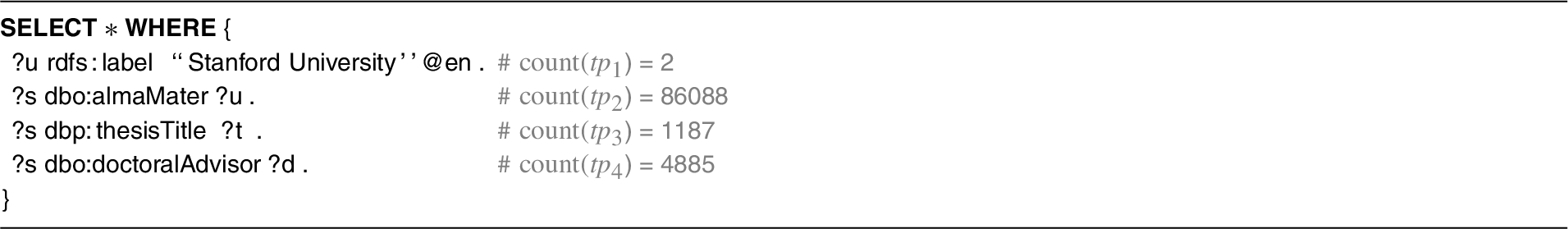
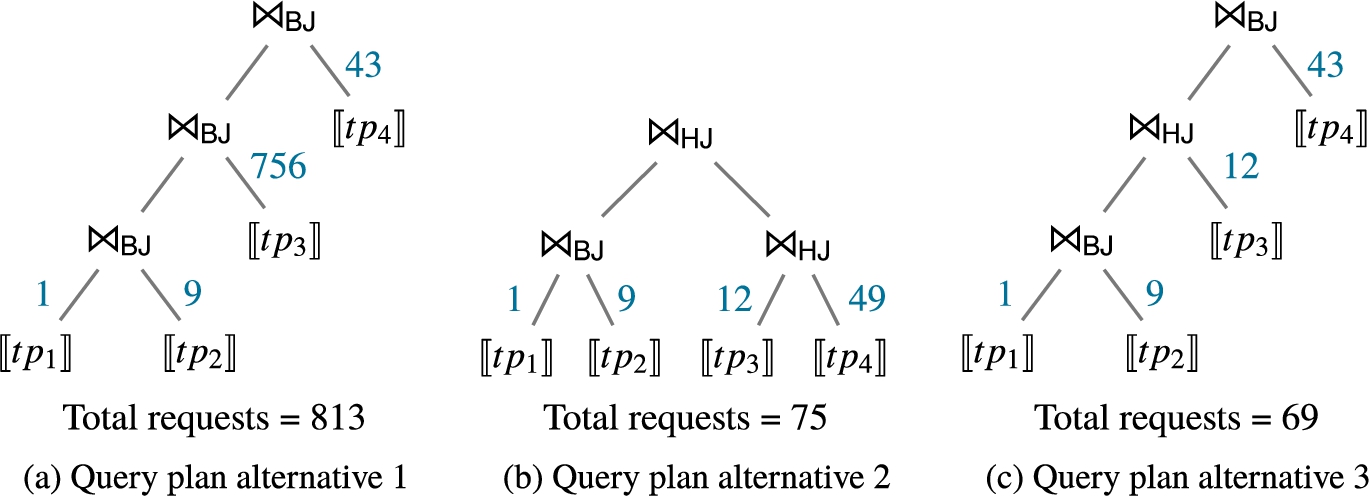
Evaluating SPARQL queries over the TPF server requires the client to obtain efficient query plans that minimize the query execution time, the number of requests, and the amount of data transferred. Typically, clients implement a query planning heuristic that relies on the metadata provided by the TPF server. The sort heuristics implemented by comunica sorts the triple patterns according to the number of triples they match in ascending order and places Nested Loop Joins (NLJs) as the physical operators [27]. Evaluating the query over the TPF server using comunica-sparql33 requires the client to perform 813 requests to obtain the 29 results of the query. The corresponding physical query plan is shown in Fig. 1(a), where the number of requests is indicated on the edges. The client performs 4 requests to obtain the statistics (counts) on the triple patterns, and thereafter, it executes the plan with 809 requests, leading to a total of 813 requests. An alternative query planning heuristic is implemented in the network of Linked Data Eddies (nLDE)44 which is another client for TPF servers. The query planning heuristic builds bushy plans around star-shaped subqueries and places Nested Loop Join or Symmetric Hash Join (SHJ) operators such that the estimated number of requests is minimized [1]. To this end, nLDE first performs 4 requests to obtain the count values of the triple patterns and thereafter, builds the bushy query plan as shown in Fig. 1(b). The execution of the query plans requires 71 requests, leading to a total of 75 requests. When inspecting the query in detail, we observe that neither comunica-sparql nor nLDE finds the query plan which minimizes the number of requests to be performed. The optimal plan is shown in Fig. 1(c) and it requires a total of 69 requests only: 4 requests to obtain the counts and 65 requests to execute the plan. The number of requests in the query plan can be reduced by sorting the triple patterns similar to comunica by ascending count values. Furthermore, placing the appropriate physical join operators according to the join cardinalities of the sub-plans minimizes the number of requests.
The example query showcases the challenge for heuristics to devise efficient query plans based only on the count statistic provided by the TPF servers. In the query, the subject-object join of triple patterns
Fig. 1.
Three alternative query plans for the SPARQL query from Listing 1. Indicated on the edges are the number of requests to be performed according to the corresponding join operators: nested loop join (NLJ) and symmetric hash join (SHJ).
In addition, adaptive query processing strategies [10] allow to eradicate potential query planning errors by adapting the join processing during query plan execution. Take for example the query plan in Fig. 1(a) which requires a large number of requests by probing each individual tuple from
Our motivating example illustrates how efficient client-side query processing over TPF server can be achieved by (i) obtaining efficient query plans that are less prone to cardinality estimation errors, and (ii) adapting the join strategy during query execution. In Section 4, we present our approaches for robust query planning that not only considers the best-case scenario but also an average-case scenario when determining an efficient query plan. Moreover, in Section 5, we present the concept of Polymorphic Join Operators which are able to adapt their join strategy during query execution.
3.Background and related work
Different cost models and adaptive techniques have been proposed in federated SPARQL query engines. Therefore, we first present related work on federated SPARQL query processing (§3.1). Thereafter, we present the planning techniques implemented by client-side query processing for Linked Data Fragments (§3.2). Finally, we present adaptive and robust query processing approaches from the area of relational databases which address estimation errors in query planning and query execution (§3.3).
3.1.Federated SPARQL query processing
A variety of cost models [9,12,23–25] and adaptive query processing approaches [2,20] have been proposed to employ efficient federated SPARQL query processing. DARQ [24] implements a cost model to reduce the amount of data transferred and the number of transmissions. The cost estimation functions for nested loop joins and bind joins rely on join cardinality estimations derived from statistical information from the service descriptions of the federation members. The optimizer uses Iterative Dynamic Programming (IDP) to obtain an efficient query plan. The federated engine SPLENDID [12] also implements a cost model to devise efficient plans. The cost model incorporates the network communication based on the estimated number of tuples to be transferred for either a bind or a hash join operator. Join cardinalities are estimated using precomputed indices based on VoID descriptions. The optimizer uses Dynamic Programming (DP) to find the cost-optimal plan. The cost model in SemaGrow [9] incorporates the costs for querying endpoints, transferring tuples, and processing them locally. The cardinality estimations for computing these costs rely on detailed statistics including the number of distinct subjects, predicates, and objects for a given triple pattern. The query plan optimizer uses DP to enumerate the space of possible join plans and prunes inferior plans. The cost function of Odyssey [23] is only based on the cardinalities of intermediate results to favor plans that produce fewer intermediate results. The cardinalities of intermediate results are estimated using characteristics sets statistics of the federation members, and DP is applied to enumerate alternative join orders for the subexpressions. CostFed’s [25] cost model also relies on detailed data summaries to estimate the cardinalities of subexpressions. The cost model is tailored to physical query plans with symmetric hash joins and bind joins. The optimizer follows a greedy-heuristic to incrementally build sub-plans with minimal cardinalities.
Federated SPARQL query processing approaches that focus on runtime adaptivity include ANAPSID [2] and ADERIS [20]. ANAPSID [2] is a federated SPARQL query engine that adapts to data availability and runtime conditions of endpoints to hide delays from users. The engine implements a query planner based on adaptive sampling and two non-blocking join operators that aim to produce query results even in the case that SPARQL endpoints get blocked. The ADERIS system [20] focuses on adaptive join ordering for federated SPARQL queries. The system relies on basic statistics (predicates per source) for an initial decomposition of the query. In contrast to a static query plan, ADERIS adapts the join order during query execution using a cost model that uses the cardinalities and selectivities determined during runtime.
Similar to our work, existing federated querying approaches [9,12,23–25] implement cost models for comparing alternative query plans. The cost models typically combine local processing and network communication cost and consider different join operators. However, they rely on fine-grained cardinality estimations that are based on detailed statistics about the data sources. Moreover, the optimizers are able to employ different plan enumeration approaches, such a DP, since typically the search space for federated plans is smaller as they work with subexpressions which are typically composed of several triple patterns and other operators. Similar to the Polymorphic Join Operators, ANAPSID [2] also focuses on intra-operator adaptivity but the join operators adapt to delayed or bursty data traffic rather than cardinality estimation errors. In contrast to our work, ADERIS [20] implements inter-operator adaptivity and the cost model relies on cardinality and selectivity statistics produced during the query execution.
3.2.Linked data fragments and clients
Linked Data Fragments (LDF) are interfaces for accessing and querying RDF graphs on the Web [28]. A central difference between these interfaces is their expressivity and the metadata they provide [15,17], resulting in different client-side query processing approaches for LDF interfaces. The original Triple Pattern Fragment (TPF) client [28] supports the evaluation of SPARQL queries over TPF servers and implements a heuristics to process the query which tries to minimize the number of requests. The TPF client implements non-blocking operators and the join order is given by sorting the triple patterns according to their cardinality. The triple pattern with the smallest estimated number of matches is evaluated and the resulting solution mappings are used to instantiate variables in the remaining triple patterns. This procedure is executed continuously during runtime until all triple patterns have been evaluated. Comunica [27] is a modular query engine that supports SPARQL query evaluation over heterogeneous interfaces including TPF servers. The client is embedded in the Comunica framework which aims to provide a research platform for SPARQL query evaluation to support the development of modular, web-based query engines. Comunica currently supports two heuristic-based configurations. The sort configuration sorts all triple patterns according to the metadata and joins them in that order similar to [28]. The smallest configuration does not sort the entire BGP but selects the triple pattern with the smallest estimated count on every recursive evaluation call. The network of Linked Data Eddies (nLDE) [1] is an adaptive client-side SPARQL query engine over TPF servers. The query optimizer in nLDE builds star-shaped groups (SSG) and joins the triple patterns by ascending cardinality. The optimizer places either symmetric hash join or nested loop join operators to minimize the expected number of requests that need to be performed. Furthermore, nLDE realizes adaptivity by adjusting the routing of result tuples during the query execution according to changing runtime conditions and data transfer rates.
More expressive LDF interfaces include brTPF and smart-KG. Bindings-restricted Triple Pattern Fragments (brTPF) [14] are an extension of the TPF interface that allows for evaluating a given triple pattern with a sequence of bindings to enable more efficient bind join strategies. Given a triple pattern and sequence of bindings, the brTPF server instantiates the variables of the triple pattern with the bindings and evaluates them over the RDF graph to return the matching triples. The authors propose a heuristic-based client that builds left-deep query plans which aims to reduce the number of requests and data transferred by leveraging bind joins. Smart-KG [6] is a hybrid shipping approach which aims to balance the load between clients and servers when evaluating SPARQL queries over remote sources. The smart-KG server extends the TPF interface by providing access to compressed partitions of the graph. These partitions are based on the concept of predicate families to support the evaluation of star-shaped subexpression over the partition at the client. The smart-KG client determines which subexpressions are evaluated locally over the shipped partitions and which triple patterns should be evaluated at the server.
Finally, SaGe [22] is a query engine that supports Web preemption by combining a preemptable server and a corresponding smart client. The server supports the fragment of SPARQL which can be evaluated in a preemptable fashion. The client decomposes a query such that the resulting subexpressions can be answered by the server and it also handles the preemptable execution of the query. As a result, the evaluation of the subexpressions is carried out at the server using a heuristic-based query planner that builds left-deep plans with index loop joins.
Different from the existing LDF clients, our query planner relies on a cost model, a robustness measure, and IDP to devise efficient query plans. Specifically, we focus on the TPF interface to showcase the effectiveness of our approach, however, it can be extended to support additional LDF interfaces. For instance, by extending the probe function in our cost-model to also support brTPF with several bindings per request. In addition, more expressive LDF interfaces and their clients may also benefit from our robustness measure. For example, to devise efficient and robust query plans in the smart-KG client or the SaGe server. While existing clients implement adaptivity during runtime [1,27,28], in contrast to the Polymorphic Join Operators, these adaptive approaches do not adjust the join strategy in response to estimation errors but focus on changing the join order and tuple routing during execution.
3.3.Robust query processing in relational databases
In the realm of relational databases, various approaches address uncertainties in the statistics and parameters used in cost models. Wiener et al. [29] consider different types of robustness including (i) query optimizer robustness as the ability of the optimizer to choose good plans under unexpected conditions, and (ii) query execution robustness as the efficient execution of a given plan under different runtime conditions. Yin et al. [32] focus on the former by investigating robust query optimization methods which are robust with respect to estimation errors. Their classification of such methods includes Robust Plan Selection, which comprises approaches that select a “robust” plan which is less sensitive to estimation errors over the “optimal” plan. These approaches, for example, use probability density functions for cardinality estimations instead of single-point values [7] or define cardinality estimation intervals where the size of the intervals indicate the uncertainty of the optimizer [8]. Wolf et al. [30] propose cardinality-based and selectivity-based robustness metrics for query plans. The core idea is computing the cost of a query plan as a function of the cardinality and selectivity estimations at all edges in the plan. The robustness metrics are computed based on the slope and area under the resulting cost function.
The CROP query planner can be considered a Robust Plan Selection approach. In contrast to [7] and [8], CROP has to rely on coarse grained statistics that do not allow for computing selectivity or cardinality estimation probabilities. Similar to [30], our measure computes the robustness of query plans and selects a robust plan from a selection of the cheapest plans.
Besides robust query planning, a variety of adaptive query processing approaches [10,13] have been proposed to support query execution robustness. Similar to our work, operator replacement considers approaches, where physical operators can be replaced with a logically equivalent operator at runtime [13]. Operator replacement typically occurs due to mid-query re-optimization [10]. For example, progressive query optimization (POP) [21] adapts to cardinality estimation errors by re-optimizing the query plans potentially leading to operator replacement. To this end, POP determines validity ranges of sub-plan cardinalities that trigger query plan re-optimization if the actual cardinalities violate these ranges. Materialized views and corresponding checkpoints allow the re-optimized query plans to reuse intermediate results.
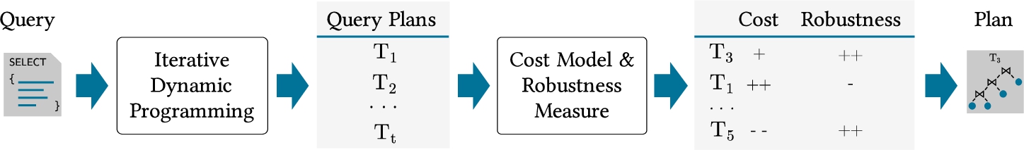
Fig. 2.
Overview of CROP.
Similarly, Rio [8] adapts to cardinality estimation errors by (i) considering the robustness of query plans during query optimization based on bounding-boxes for estimations, and (ii) creating switchable plans during the optimization phase that can be used as alternatives plans in response to estimation errors at runtime.
The proposed Polymorphic Join Operators can be considered as dynamic operator replacement. However, in contrast to [21] and [8], the Polymorphic Join Operators do not require a re-optimization of the query plan or precomputed switchable plans. Moreover, the Polymorphic Join Operators independently decide whether they adapt their join strategy solely based on runtime conditions without detailed statistics for validity ranges or bounding-boxes. This makes our proposed solution suitable for query execution over LDFs, where the engine has access only to coarse-grained statistics.
4.Robust query planning
We present CROP, a cost- and robustness-based query plan optimizer to devise efficient plans for SPARQL queries over Linked Data Fragment (LDF) servers. An overview of the approach is provided it Fig. 2. Given a SPARQL query, the query plan optimizer determines a set of alternative query plans. The efficiency and robustness of these plans are estimated by our cost model and robustness measure. Finally, the optimizer selects a query that yields an appropriate trade-off of both cost and robustness. In the following, we start by introducing the preliminaries and thereafter, present the cost model (§4.2), robustness measure (§4.3), and query planner (§4.4) in detail.
4.1.Preliminaries
The foundation of this work is the Resource Description Framework (RDF). Consider the three pairwise disjoint sets of Internationalized Resource Identifiers (IRIs) I, blank nodes B, or literals L. An RDF term is an element in
Definition 4.1
Definition 4.1(SPARQL Expression [26]).
A SPARQL expression is an expression that is recursively defined as follows.
(1) A triple pattern
(2) If
Furthermore, we denote the universe of SPARQL expression as
In the remainder of this work, we focus on query plans for BGPs to be evaluated over Linked Data Fragment (LDF) servers. An LDF server is a Web interface to access and query RDF graphs. We identify an LDF server by its IRI
Example 4.1.
The TPF server for DBpedia of our motivating example can be defined as
–
–
–
The central components of query plans for evaluating BGPs over LDF servers are its access operators. An access operator evaluates a SPARQL expression over a given LDF server by performing the necessary HTTP requests to obtain all solution mappings according to the interface.
Definition 4.2
Definition 4.2(Access Operator).
An access operator is a tuple
A join query plan defines the join order, the physical join operators, and the access operator for evaluating a BGP P in a tree structure.55
Definition 4.3
Definition 4.3(Join Query Plan).
A join query plan T is a binary tree, where the leaves
For query plan T, we denote the number of leaves as  ) and physical join operators (⋈). In addition, we indicate the join algorithm of a physical join operator by its subscript. For example, a bind join operator is denoted by
Definition 4.4
Definition 4.4(Evaluation of a Join Query Plan).
Given a query plan T, the evaluation of T is defined as 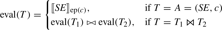
Furthermore, we define a function
Proposition 4.1.
Given an LDF interface c for RDF graph G with
The proposition follows from the algebraic equivalences defined by Schmidt et al. [26] and the fact that all expressions are evaluated over the same graph
4.2.Cost model
We now present our cost model to estimate the cost of evaluating a query plan for a basic graph pattern over an LDF server. In principle, the cost for evaluating a query plan in a decentralized scenario are determined by (i) the server cost for processing the requests (i.e., evaluating the expression) on the server, (ii) the network cost for transporting requests and responses over the network, and (iii) the client cost, for processing the tuples of the response. Specifically, determining the server and network costs is challenging in practice since they are influenced by a large number of factors, such as the server load or potential network delays. Therefore, we use the number of requests that need to be performed by an access operator as a proxy for server and network costs. Consequently, for the sake of comparability of the individual requests of the access operator and because any LDF interface (except data dumps) allows for evaluating triple patterns, we assume the subexpressions in the access operators to be triple patterns, i.e.,
In the following, we focus on the request cost for access operators for TPF servers and for the physical join operators Bind Join (BJ) and symmetric Hash Join (HJ). Given a query plan T for a conjunctive query the cost of evaluating T over LDF server c is computed as
4.2.1.Processing cost
The processing costs account for the effort of handling the tuples at the client once they have been received from the server. For instance, this includes parsing the tuples into the corresponding data structures and potentially inserting them into hash tables in the join operators. The first parameter of the cost model
In both cases, the estimated tuples produced by the join
4.2.2.Request cost
In our cost model, we use the request cost as a proxy for the network cost and the server-side cost when evaluating an expression at the server. The request cost
Access operator If a T is an access operator
Bind join The request costs of a Bind Join (BJ) are determined by the request cost for obtaining the tuples of the outer plan
In practice, there are two major reasons why this cannot be computed accurately. First, the number of tuples in
The minimum number of requests that need to be performed is given by the cardinality for
The discounting factor for BJs is computed using the parameter
The rationale for including a discount factor for the requests on the inner plan is twofold. First, since the join variables are bound by the terms obtained from the outer plan, the number of variables in the triple pattern is reduced which can reduce the cost per request. This was shown in an empirical study for TPF servers [18]. Second, for star-shaped queries, typically the number of tuples reduces with an increasing number of join operations and, therefore, the higher the BJ operator is placed in the query plan, the more likely it is that it needs to perform fewer requests in the inner plan than the estimated cardinality of the outer relation suggests. The discount factor
Symmetric hash join The request cost for the symmetric Hash Join (HJ) operator is computed based on the number of requests that need to be performed if either or both sub-plans
If both
Note that the number of requests for the HJ can be computed accurately if the true cardinalities of the expressions of the access operators are known. For example, the count metadata that provides (an estimation of) the number of triples matching a triple pattern allows for determining the number of requests accurately.
Cardinality estimation Central to our cost model are the expected number of intermediate results produced by the join operators as this number affects both the local processing and the request costs. Since we focus on query plans for BGPs, we determine the number of intermediate results by recursively applying a join cardinality estimation function to the query plan T. Given a query plan T, we estimate the cardinality as
To compute the cardinality estimation for an access operator
After presenting our cost model, we will now present the concept of robustness for query plans in order to avoid always choosing the cheapest plan merely based on these optimistic cardinality estimations.
4.3.Query plan robustness
Query planning approaches benefit from accurate join cardinality estimations to determine a suitable join order and to properly place physical operators such that the execution time of the query plan is minimized. However, estimating the join cardinalities is a challenging task, especially in the case that only basic statistics about the data are available. Addressing this challenge, we propose a robustness measure in order to determine how strongly the costs of a query plan are affected by potential cardinality estimations errors. To this end, our robustness measure compares the best-case cost of a query plan to its average-case cost. The average-case cost of a query plan is computed by using different cardinality estimation functions in the cost model to cover alternative join cardinalities. The resulting cost for each estimation function and the same query plan can be aggregated to an average cost value. Thus, a robust query plan is a plan in which the best-case cost only slightly differs from the average-case cost.
Example 4.2.
Let us revisit the query plans from our motivating example in Section 2. As we focus on query plans with access operators for the same LDF server c, for the sake of readability, we omit the access operator in the following examples, i.e.,
Table 1
Cost of query plans
| Cardinality Estimation Function | |||
| minimum | mean | maximum | |
| 5 | 43 477 | 86 951 | |
| 15 | 445 | 875 | |
Query plan
Definition 4.5
Definition 4.5(Cost ratio robustness measure).
Let T be a query plan,
That is, the cost ratio robustness (crr) of a plan is the ratio between the cost in the best-case
We extend the definition of the cost function from Section 4.2 to capture the average-case cost of a query plan by including the cardinality estimation functions applied to each join operator. Let
Definition 4.6
Definition 4.6(Best-case cost).
The best-case cost for a query plan T is defined as
In other words, at every join operator in the query plan, we use the minimum cardinality of the sub-plans to estimate the join cardinality. This is identical to the estimations used in our cost model. Note that while in principle the cardinality for very selective joins can even be lower than the minimum, it still provides an optimistic estimation for computing the best case cost. The computation of the average-case cost requires applying different combinations of such estimation functions at the join operators.
Definition 4.7
Definition 4.7(Average-case cost).
Given a set of m estimation functions
By applying a variety of cardinality estimation functions, different join selectivities can be reflected in the average-case cost. We empirically tested different sets of estimation functions in F and found that the following functions yield suitable estimations for computing the average-case cost:
The rationale for selecting these functions is to capture different join selectivities based on the cardinality estimations of the sub-plans to be joined. The function
Example 4.3.
Let us consider the query plan alternative 1 from our motivating example (cf. Fig. 1). In this example, the join  is a s-o join and all other joins are s-s joins. As a result, to compute the average case cost, the alternative estimation functions in F are applied to estimate
  . Based on these four alternative cardinality estimations, the minimum cardinality (cf. Eq. (4)) is used to estimate the cardinality of the remaining joins (as they are s-s joins). With these cardinality estimation alternatives, the cost of the query plan is computed which results in four different cost estimations. Finally, to obtain the average-case cost value, the median of those four cost estimations is computed.
4.4.Query plan optimizer
After presenting our cost model and robustness measure, we now present our optimizer that combines both aspects. Introducing the concept of robustness for query plans in addition to their cost yields two major questions: (i) in which cases should a more robust plan be chosen over the cheapest plan, and (ii) which alternative robust plan should be chosen instead of the cheapest plan? To this end, we propose a query plan optimizer that combines both aspects. Its parameters allow for defining the sensitivity of when a robust plan should be selected and also which alternative plan should be chosen over the cheapest plan. The query plan optimizer follows three main steps:
1. Obtain a selection of alternative query plans using Iterative Dynamic Programming (IDP).
2. Assess the robustness of the cheapest plan.
3. If the cheapest plan is not considered to be robust enough, find an alternative robust query plan.
Algorithm 1:
CROP query plan optimizer
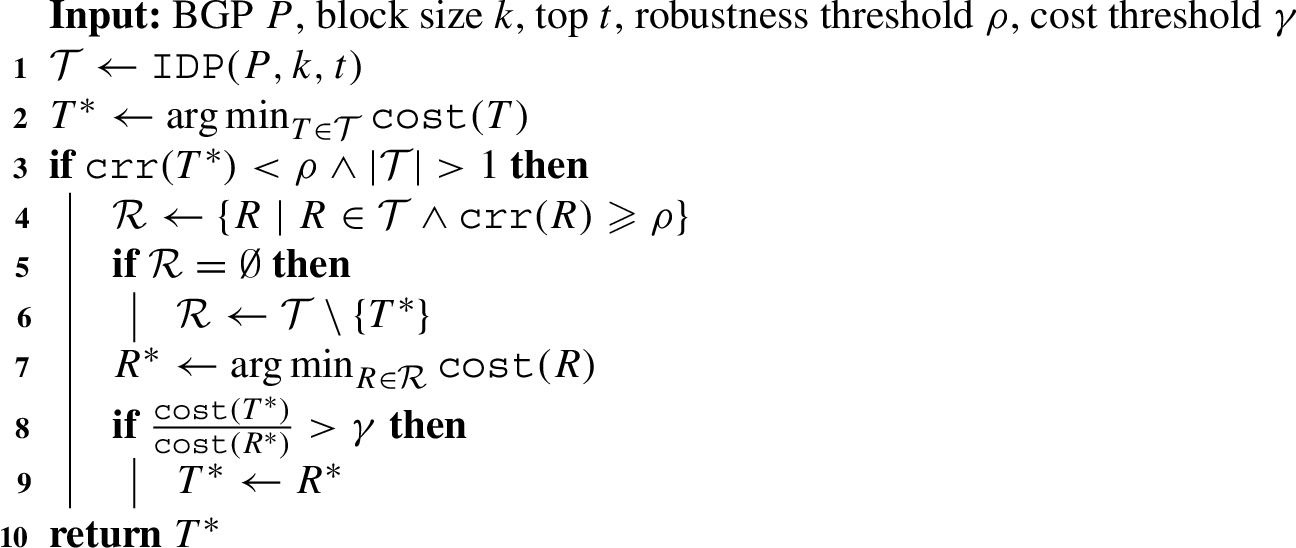
The query plan optimizer is detailed in Algorithm 1. Given a BGP P, the query planner determines the best query plan
Example 4.4.
Consider the query for the motivating example and
Given the set of t candidate query plans
Theorem 4.1.
With the number top plans t and the set of estimation functions F constant, the time complexity of the query plan optimizer is for a BGP P with n triple patterns in the order of
Case I:
Case II:
Proof.
The time complexity of the query plan optimizer is given by the IDP algorithm and computing the average-case cost in the robustness computation. Kossmann and Stocker [19] provide the proofs for the former. For the latter, given
Case I: For
Case II: For
5.A new class of adaptive join operators
We now present a new class of adaptive join operators which we call Polymorphic Join Operators. The goal of these operators is to improve the runtime efficiency by adapting the join strategy during the execution of a query plan. In particular, these operators adapt to potential join cardinality estimation errors of the planner to achieve an additional level of robustness during query execution.
A central task of the query planner is deciding on the appropriate physical join operators that maximize the query plan’s efficiency with respect to the runtime and number of requests. The efficiency depends on the join strategies implemented by the operators and the number of intermediate results they need to process. Based on join cardinalities estimations of the sub-plans, the query planner decides to place operators that implement different join strategies (e.g., bind join, hash join, etc). A client following the optimize-then-execute paradigm would then execute the resulting query plan. However, this approach does not allow for adapting to potential estimations errors of the planner which can lead to sub-optimal join strategies. Alternatively, the client could support intra-operator adaptivity aiming to support robust query execution. To this end, we propose two new operators in this class of adaptivity, namely a Polymorphic Bind Join and a Polymorphic Hash Join operator. For the sake of simplicity, we present the operators with a bindings block size equal to one, that is a single tuple is probed during the bind join phase. The operators can easily be extended to support larger block sizes for more expressive LDF interfaces.66
5.1.Polymorphic bind join
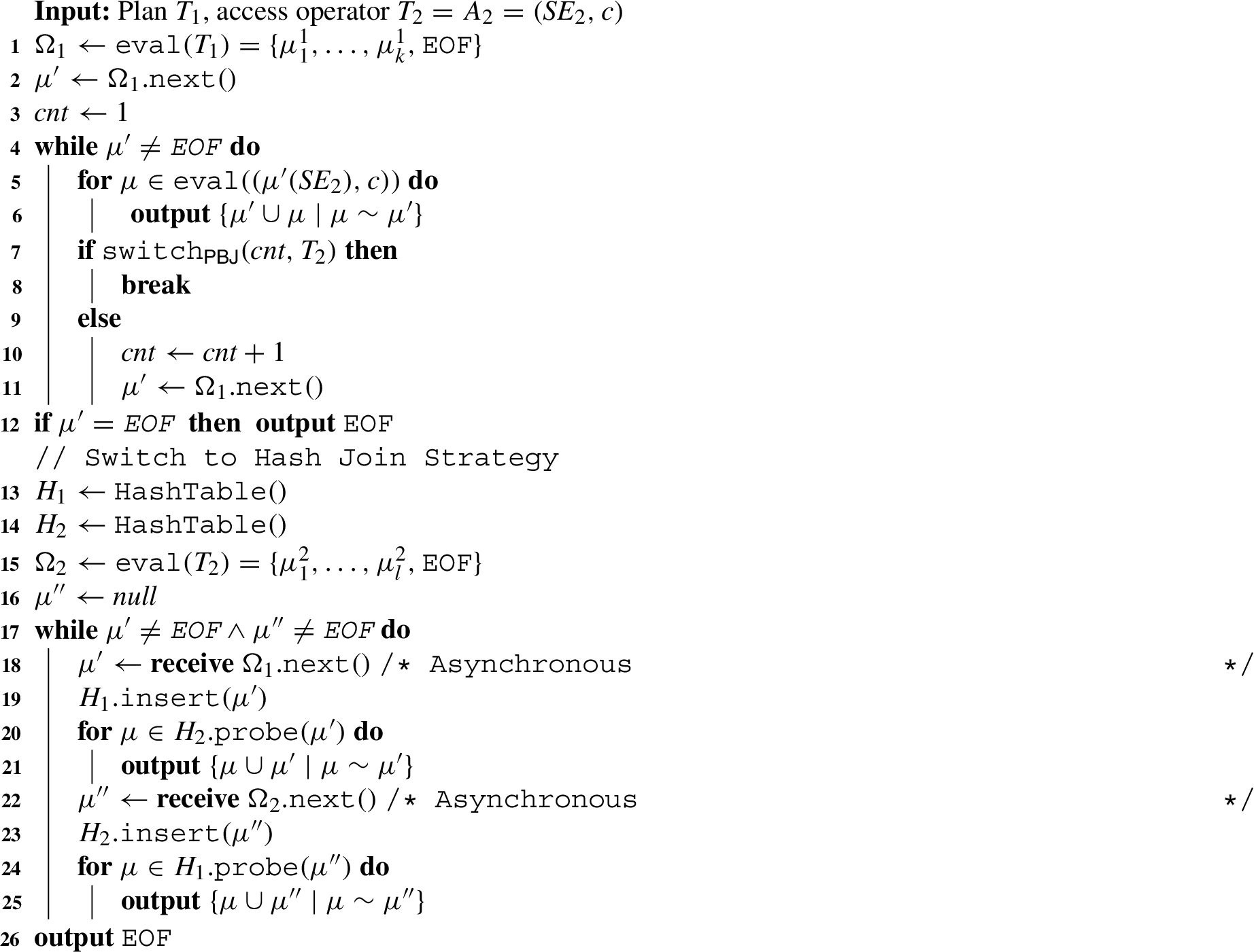
The Polymorphic Bind Join (PBJ) is a physical join operator that can switch its join strategy during query execution from a bind join to a hash join strategy. We denote the PBJ by
The PBJ operator is outlined in Algorithm 2. The operator receives a stream of tuples from the evaluation of the sub-plan
Adding the parameter
In the case that the operator decides to switch its join strategy (Line 9), it terminates the loop of the bind join. Thereafter, the operator sets up two hash tables (Line 14 and 15) and starts evaluating
Algorithm 2:
Polymorphic bind join
Example 5.1.
Let us consider the query plan from our motivating example shown in Fig. 1(a) that is evaluated over the DBpedia TPF server with a page size of 100. We focus on the second join operator
Parameters for the PBJ The PBJ follows a simple heuristic-based decision rule to decide whether it should switch its join strategy. This is due to the fact that it cannot assess how many tuples in
In other words, the PBJ decides correctly if it switches to a hash join operation as long as the access requests for
Example 5.2.
We consider the query plan from Fig. 1(a) with PBJ operators and focus on the second join operator
1. If
2. If
3. If
Correctness of the PBJ We show that the Polymorphic Bind Join operator produces correct solution mappings according to the SPARQL set semantics [26].
Theorem 5.1.
Given an RDF graph G, an LDF interface c with
The intuition of the operator’s correctness is as follows. If the operator does not switch its join strategy, it operates as a regular bind join operator producing correct results. In the case that it switches from the bind join strategy to the hash join strategy, there are still tuples from
Proof.
We demonstrate the correctness of the operator
Completeness: We assume that the
Let us consider a solution mapping μ, such that
Case I:
Case II:
Soundness: We assume that the
To this end, we consider a solution mapping μ, such that
5.2.Polymorphic hash join
We now introduce the Polymorphic Hash Join (PHJ), which is the complement of the PBJ. The PHJ enables adaptivity by switching its join strategy from a hash join to a bind join during query execution. We denote the PHJ by
Algorithm 3:
Polymorphic hash join
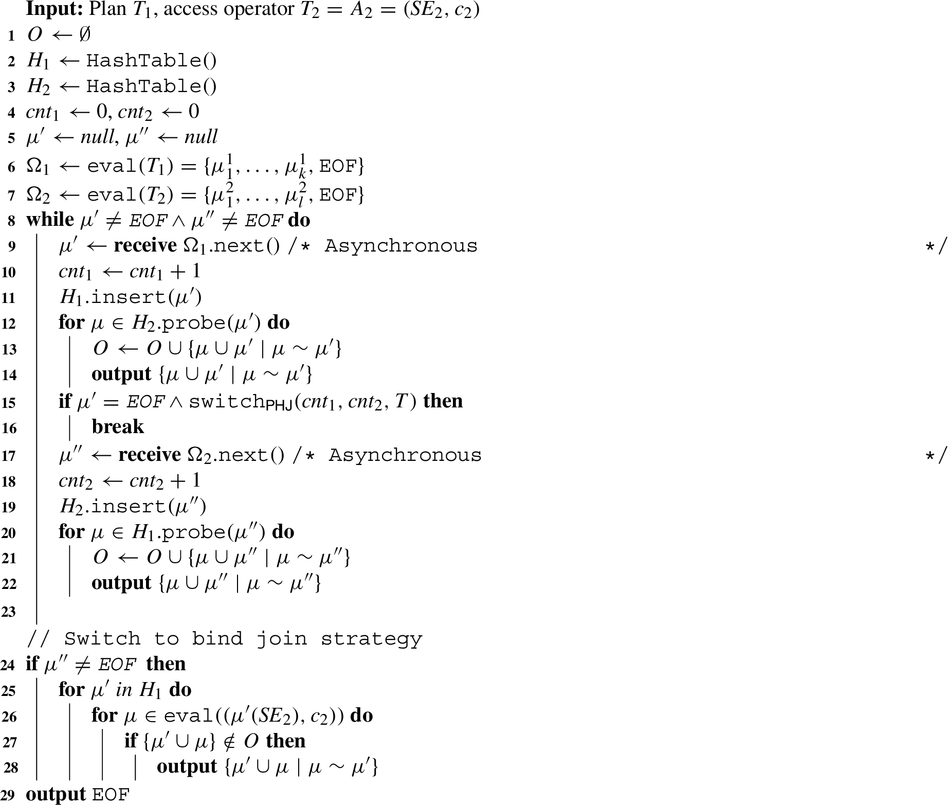
The PHJ operator is outlined in Algorithm 3. In the first phase, the operator follows a non-blocking, symmetric hash join strategy as long as the operator receives tuples from
The parameter
In the case that the PHJ decides to switch to the bind join, it terminates the hash join phase (Line 16). Thereafter, in the bind join phase, the operator probes all tuples from
Optimality condition for the PHJ For the PHJ there is an optimal parameter
Proposition 5.1.
For a query plan
In other words, if
If we assume that all requests are equal in terms of response time, we have that
Correctness of the PHJ We now show that the Polymorphic Hind Join operator produces correct solution mappings according to the SPARQL set semantics [26].
Theorem 5.2.
Given an RDF graph G, an LDF interface c with
The intuition of the operator’s correctness is as follows. If the operator does not switch its join strategy, it operates as a regular hash join operator producing a correct result set. The operator considers switching from the hash join strategy to the bind join strategy when all tuples from
Proof.
We prove the correctness of the operator
Completeness: The first case is that the
Let us consider a solution mapping μ, such that
Case I: The operator does not switch the operation, i.e.,
Case II: The operator switches the operation to the bind join strategy. This can only be the case if all solution mappings from
In both cases, the solution mapping μ is produced by the PHJ. This contradicts the assumption that
Soundness: The second case is that the
This means there is a solution mapping μ, such that
The first case is that
The second case is that μ is produced twice (i.e., a spurious duplicate) when the operator processes
5.3.Summary
We introduced a new class of adaptive join operators that are able to switch their join strategy during the execution of a query plan. In particular, we presented two instances from this class: the Polymorphic Bind Join (PBJ) and the Polymorphic Hash Join (PHJ). These operators allow for switching their join strategy from a bind join to a hash join and vice versa. While we presented PBJ and PHJ operators probe a single tuple in the bind join phase, both operators can easily be extended to handle several bindings per request (binding block size > 1). Moreover, the proposed operators can be further optimized by leveraging the query planner and the properties of the LDF interface. The query planner could determine the sensitivity of individual operators according to estimated cardinalities and probabilities of estimation errors. In addition, the operators could leverage the properties of the underlying LDF interface. For example, in the case that the solution mappings are sorted (e.g., for a TPF server with an HDT backend), the operators could use the order to reduce the number of requests after switching the join strategy. In addition, the PHJ could be extended in two ways. First, instead of keeping all produced tuples in the set O to avoid producing duplicate solution mappings, the operator could also check during the bind join phase, whether the tuples are in the hash table
6.Evaluation
In this experimental evaluation, we investigate the effectiveness of our two approaches for robust query processing over Linked Data Fragments. As previously mentioned, we evaluate the approaches using the example of Triple Pattern Fragment (TPF) servers. We investigate the effectiveness of the proposed query planning approach CROP and the impact of the adaptive join operators PBJ and PHJ on two different benchmarks with a fine-grained analysis of the results.
6.1.Experimental setup
Datasets and queries As the basis for our evaluation, we focus on two different datasets and corresponding benchmark queries that have also been used in previous evaluation for LDF clients [1,6,14,22,27,28]. First, we use a synthetic RDF graph and benchmark queries from the Waterloo SPARQL Diversity Test Suite (WatDiv) [4]. Specifically, we generated a dataset with scale factor = 100 and the corresponding default queries with query-count = 5 resulting in a total of 88 distinct queries from query categories, namely, 25 linear queries (L), 35 star queries (S), 25 snowflake-shaped queries (F) and 3 complex queries (C). The second benchmark is taken from the evaluation of nLDE99 and is based on the real-world RDF graph of DBpedia 2014 [1]. The benchmark consists of two subsets of queries. The first subset, Benchmark 1 (BM 1), consists of 20 non-selective queries composed of basic graph patterns with up to 14 triple patterns that produce a large number of intermediate results. The second subset, Benchmark 2 (BM 2), consists of 25 more selective queries from the domains Historical, Life Science, Movies, Music, and Sports. The number of queries per category as well as statistics on the number of answers and number of triple patterns for the queries of benchmarks is provided in Table 2. In addition, to showcase the benefits of combining the cost model with robustness in the query plan optimizer on different RDF graphs, we designed an additional test-set with 10 queries for 3 RDF graphs that include either a s-o and or an o-o join and 3-4 triple patterns. We used the RDF graphs DBpedia 2014, GeoNames 2012, and DBLP 2017 for which we obtained the HDT files from the RDF-HDT website.1010
Table 2
Properties of the benchmark queries
| # | # Answers | # Triple Patterns | |||||
| min | max | median | min | max | |||
| WatDiv | C | 3 | 2 | 417 029 | 20 | 6 | 10 |
| F | 25 | 0 | 58 | 8 | 6 | 9 | |
| L | 25 | 0 | 239 | 47 | 2 | 3 | |
| S | 35 | 0 | 320 | 4 | 3 | 9 | |
| nLDE | BM 1 | 20 | 2 | 45 655 205 | 7131 | 4 | 14 |
| BM 2 | 25 | 2 | 1768 | 19 | 3 | 5 | |
Implementation We implemented CROP1111 on top of the nLDE client4, which is implemented in Python 2.7.13. We implemented our cost model, robustness measure, and query plan optimizer, such that the resulting physical query plans can be executed using nLDE. We used the default of 2 eddy operators and do not consider the routing adaptivity features of nLDE, that is, we select no routing policy for the execution. We deployed the TPF server with an HDT backend [11] using the Server.js v2.2.31212 implementation. We set the number of workers for the TPF server to 5. All experiments were executed on a Debian Jessie 64 bit machine with CPU: 2× Intel(R) Xeon(R) CPU E5-2670 2.60 GHz (16 physical cores), and 256 GB RAM. The queries were executed three times in all experiments. The timeout was set to 900 seconds for the experiments to set the parameters for CROP (δ, k, γ, and ρ). For all the remaining experiments, we set a runtime timeout of 600 seconds.
Evaluation metrics We consider the following query execution metrics:
(i) Runtime: Elapsed time in seconds spent by a query engine to complete the evaluation of a query measured in seconds. In the implementation of CROP, we distinguish between the optimization time spent by the query planner to obtain a query plan and the execution time to execute the plan.
(ii) Number of Requests: Total number of requests submitted to the server during the query execution including query planning.
(iii) Number of Answers: Total number of answers produced during query execution.
(iv) Diefficiency: Continuous efficiency as the answers are produced over time [3].
We provide all results of our experimental study in our supplemental material on Zenodo.1313
Table 3
Cost-model: impact of the δ-parameter of the height discount factor for the Bind Join (BJ) on the query plan efficiency (runtime and requests), percentage of BJs and bushy plans. Best efficiency values are indicate in bold
| δ | WatDiv | nLDE BM | ||||||
| Runtime (s) | Requests | BJs | Bushy Plans | Runtime (s) | Requests | BJs | Bushy Plans | |
| 0 | 255.0 | 24 039 | 50% | 2% | 1300.75 | 24 702 | 34% | 10% |
| 1 | 267.01 | 30 133 | 61% | 2% | 588.74 | 24 743 | 39% | 10% |
| 2 | 224.6 | 30 708 | 66% | 0% | 330.99 | 27 184 | 44% | 10% |
| 3 | 222.15 | 29 907 | 72% | 0% | 221.27 | 36 154 | 54% | 10% |
| 4 | 221.26 | 29 587 | 74% | 0% | 182.86 | 36 497 | 59% | 10% |
| 5 | 236.55 | 32 933 | 74% | 2% | 196.83 | 40 082 | 67% | 5% |
| 6 | 215.22 | 32 659 | 73% | 5% | 200.95 | 42 587 | 71% | 5% |
| 7 | 211.72 | 32 651 | 74% | 5% | 202.02 | 42 586 | 71% | 5% |
6.2.Robust query planning
We start by evaluating the proposed cost model, robustness measure, and corresponding query planner. First, we focus on the height discount factor for the cost model and the block size k for the IDP algorithm. Second, we focus on the cost and robustness threshold values of the query planner. Finally, we compare the resulting parameterization for CROP to the state-of-the-art clients for TPF servers. In order to determine how well the parameter settings generalize, we randomly selected a subset of the queries from the benchmarks to set the parameters but compare our approach to the state of the art for all benchmark queries. From the 88 WatDiv Benchmark queries, we randomly selected 2 queries per subgroup (L1-L5, F1-F5, S1-S7, C), resulting in 36 queries total. For the nLDE benchmark, we randomly chose 10 queries from BM 1 and 2 queries per domain from BM 2, resulting in 20 queries total.
Cost model and IDP parameters We start by investigating how the parameter settings of the cost model affect the efficiency and structure of the query plans obtained by the planner. We begin with the parameter δ which determines the impact of the height discount factor (Eq. (3)). We consider the following settings:
Regarding the efficiency of the query plans, we observe that an increase in the δ values yields a reduction of query runtimes. In particular, the lowest runtime for the WatDiv benchmark are observed for
Even though we can observe a similar impact of the δ value on the percentage of BJs in the query plans, the shape of the query plans differs in the two benchmarks. When considering the percentage of bushy plans, we find that in the WatDiv benchmark fewer bushy plans are obtained and the best results in the nLDE benchmark are observed with a higher bushy plan ratio. These results show that, on the one hand, the δ parameter not only affects the type of join operators placed in the plan but also their shape. Based on the previous observations, we set
Next, we focus on the parameterization of the IDP algorithm. Specifically, investigate how the block size k impacts both times for the planner to devise these plans (optimization time) and the efficiency of their execution (execution time and the number of requests). We set the number of top plans kept by the IDP to
Fig. 3.
IDP: impact of the different block sizes in the IDP algorithm on the execution time, optimization time, and number of requests.
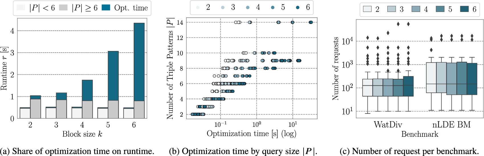
The results show that for small queries (
The optimization times (log-scale) with respect to the query size are shown in Fig. 3(b), where the block size is indicated in color. The results show the impact of the number of triple patterns in the query on the optimization time. Especially, for large block sizes
Finally, we look at the distribution of the number of requests for the different benchmark and block sizes as shown in Fig. 3(c). We can observe that for the WatDiv benchmark, the number of outliers increases, especially with
CROP query optimizer parameters The previous experiments focused on determining appropriate parameters for the cost model. We now focus on the parameters for the proposed query optimizer (cf. Algorithm 1), namely the robustness threshold ρ and the cost threshold γ. The robustness threshold ρ defines whether an alternative plan should be considered. The cost threshold γ limits the alternative plans to those which are not considered too expensive with respect to the cheapest plan. We tested all 25 combinations of
Table 4
Mean runtime, mean number of requests, and the number of robust plans (
| γ | |||||||||||||||
| Runtime | Requests | Runtime | Requests | Runtime | Requests | Runtime | Requests | Runtime | Requests | ||||||
| WatDiv Benchmark | |||||||||||||||
| 0.1 | 87.88 | 20 796 | 6 | 89.04 | 20 796 | 6 | 96.47 | 21 504 | 6 | 97.31 | 21 643 | 6 | 338.30 | 26 395 | 8 |
| 0.3 | 87.79 | 20 796 | 6 | 89.68 | 20 796 | 6 | 194.62 | 30 078 | 2 | 196.18 | 30 217 | 2 | 196.45 | 30 217 | 2 |
| 0.5 | 195.14 | 30 078 | 2 | 195.15 | 30 078 | 2 | 196.77 | 30 078 | 2 | 197.63 | 30 217 | 2 | 197.45 | 30 217 | 2 |
| 0.7 | 194.41 | 30 078 | 2 | 193.61 | 30 078 | 2 | 196.47 | 30 078 | 2 | 194.97 | 30 085 | 0 | 195.29 | 30 085 | 0 |
| 0.9 | 195.19 | 30 078 | 2 | 192.97 | 30 078 | 2 | 194.84 | 30 078 | 2 | 195.77 | 30 085 | 0 | 194.49 | 30 085 | 0 |
| nLDE Benchmark | |||||||||||||||
| 0.1 | 291.45 | 31 465 | 1 | 303.14 | 49 925 | 2 | 303.95 | 49 925 | 2 | 304.31 | 49 925 | 2 | 384.13 | 58 092 | 3 |
| 0.3 | 293.19 | 31 465 | 1 | 303.29 | 49 925 | 2 | 301.46 | 49 925 | 2 | 299.85 | 49 925 | 2 | 302.20 | 49 925 | 2 |
| 0.5 | 290.03 | 31 465 | 1 | 196.19 | 35 783 | 1 | 196.01 | 35 783 | 1 | 196.82 | 35 783 | 1 | 195.37 | 35 783 | 1 |
| 0.7 | 290.84 | 31 465 | 1 | 196.67 | 35 783 | 1 | 196.28 | 35 783 | 1 | 198.50 | 35 783 | 1 | 196.26 | 35 783 | 1 |
| 0.9 | 289.72 | 31 465 | 1 | 195.78 | 35 783 | 1 | 197.67 | 35 783 | 1 | 196.06 | 35 783 | 1 | 197.13 | 35 783 | 1 |
Fig. 4.
Custom testset: runtime, number of requests, number of answers, and query plan robustness for the 10 queries of the custom benchmark. Results compare CROP without robustness (
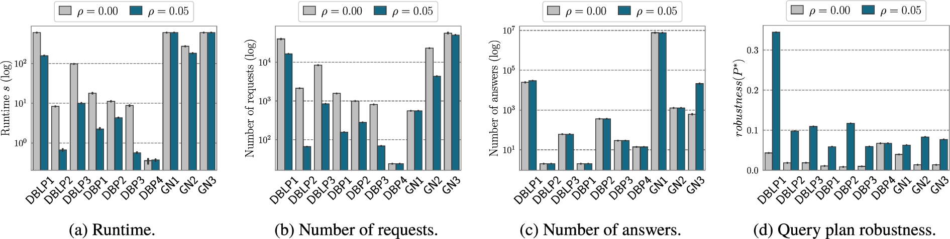
For the WatDiv benchmark, the results show that the best performing query plans are obtained for parameter values
Next, we study the effectiveness of our query planning approach in identifying efficient alternative robust plans using the 10 queries from our custom test-set. We keep the parameters from the previous experimental evaluations and compare the configuration of our planner with
Comparison to the state of the art After the intrinsic evaluation of our approach and determining appropriate parameters for the query optimizer, we now compare CROP to state-of-the-art TPF clients. Specifically, we compare CROP to nLDE [1] and Comunica [27].
Table 5
Comparison to the state of the art
| Timeout [%] | ||||||
| WatDiv | CROP | 2.12 | 0.68 | 375 | 419 448 | 0 |
| nLDE | 9.01 | 0.84 | 862 | 419 448 | 0 | |
| Comunica | 6.98 | 2.76 | 1572 | 419 448 | 0 | |
| nLDE BM | CROP | 58.14 | 0.89 | 4520 | 2 969 457 | 6 |
| nLDE | 77.15 | 0.77 | 3897 | 6 616 570 | 9 | |
| Comunica | 84.28 | 4.67 | 9234 | 423 904 | 10 |
In contrast to the previous experiments, we evaluate the clients using all queries from both benchmarks and set the timeout to 600 seconds. Table 5 summarizes the results, where the mean (
Fig. 5.
Comparison to the state of the art: mean query runtimes of Comunica, nLDE, and CROP for the different benchmarks and query categories.
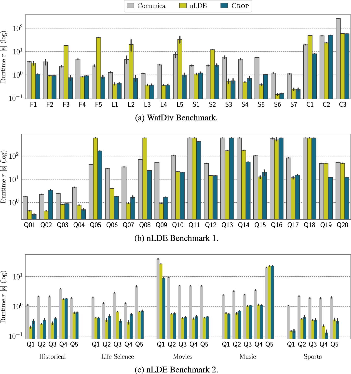
Considering the individual runtimes per query group of the WatdDiv benchmark (Fig. 5(a)), we observe that CROP, in general, exhibits very good performance in terms of runtime in the majority of the cases. Overall, CROP yields the lowest runtimes with the lowest number of requests (Table 5). Combining these observations, the results suggest that the query plans obtained by CROP find a balance between the left-deep plans (i.e., Comunica) and the bushy plans (i.e., nLDE) for the WatDiv benchmark. Finally, none of the clients reach the timeout and consequently, all clients produce complete answers.
Next, we focus on the nLDE Benchmark, for which the runtimes are detailed in Fig. 5(b) and Fig. 5(c). The runtime results for the nLDE Benchmark 1 reveal a similar performance of CROP as in the WatDiv benchmark. While CROP performs best in
Summarizing the experimental study on our cost- and robustness-based query plan optimizer CROP, we examined how the parameters of the cost model and the planner impact the query plans and compared our approach to state-of-the-art TPF clients. The results show that the height discount factor and the block size of the IDP allow the query planner for obtaining query plans that find a balance of runtime, the number of requests, and optimization time. The cost and robustness thresholds enable the query planner to determine when and which alternative robust plan should be selected, in the case that the cheapest plan is not considered to be robust enough. Finally, comparing CROP to state-of-the-art TPF clients, we found that CROP outperforms the existing approaches in the majority of cases by exploring and devising appropriate query plans without following a fixed heuristic that either builds left-deep plans (Comunica) or bushy plans (nLDE).
6.3.Polymorphic join operators
We now evaluate the proposed Polymorphic Join operators and investigate how this novel intra-operator adaptivity affects the query plan executions.
Planning approaches In order to understand the effectiveness of the adaptive PBJ and PHJ, we determine their impact on a variety of query planning approaches. As a result, we are able to examine how different planning methods can benefit from the adaptive operators during the query plan execution. Specifically, we focus on three query planning approaches: a left-deep planner, the nLDE planner, and CROP. Similar to Comunica’s sort heuristics, the left-deep planner (LDP) obtains query plans by sorting the triple patterns by increasing count values and builds left-linear plans according to this join order. We consider three different variants of the planning approach, which differ in the join strategies they implement. LDP (HJ) supports hash joins only, LDP (BJ) supports bind joins only, and LDP (BJ + HJ) supports both hash and bind joins. The LDP (BJ + HJ) uses an optimistic join cardinality estimation function (the minimum) and places either a hash join or a bind join based on the resulting estimated number of requests.1515 Additionally, we also use the nLDE planning approach that builds bushy-plans around star-shaped subqueries, and the CROP query planner with the parameter configuration from the previous experiments (
Table 6
Overview of the polymorphic join operators for the different benchmarks and planning approaches. Listed are the mean (
| WatDiv | nLDE BM | ||||||||||||
| LDP (HJ) | Baseline | 37.29 | 15.81 | 1961 | 375 163 | 0% | 0% | 176.46 | 22.77 | 2899 | 2 378 020 | 0% | 0% |
| PHJ | 10.86 | 1.84 | 651 | 16 202 | 0% | 41% | 112.92 | 1.6 | 2615 | 2 291 301 | 0% | 22% | |
| LDP (BJ) | Baseline | 12.91 | 2.95 | 1859 | 419 448 | 0% | 0% | 80.0 | 7.91 | 9561 | 1 389 673 | 0% | 0% |
| PBJ | 2.19 | 0.78 | 298 | 419 448 | 33% | 0% | 87.75 | 1.56 | 2683 | 2 184 025 | 66% | 0% | |
| LDP (BJ + HJ) | Baseline | 6.48 | 1.18 | 611 | 419 448 | 0% | 0% | 62.77 | 0.87 | 1478 | 2 369 838 | 0% | 0% |
| PBJ | 3.95 | 1.07 | 395 | 419 448 | 6% | 0% | 85.1 | 0.88 | 1676 | 1 785 498 | 7% | 0% | |
| PHJ | 4.69 | 0.71 | 499 | 419 448 | 0% | 16% | 62.71 | 0.86 | 1477 | 2 404 440 | 0% | 0% | |
| PBJ + PHJ | 2.11 | 0.7 | 283 | 419 448 | 6% | 16% | 85.26 | 0.93 | 1675 | 2 421 653 | 7% | 0% | |
| nLDE | Baseline | 9.01 | 0.84 | 862 | 419 448 | 0% | 0% | 77.15 | 0.77 | 3897 | 6 616 570 | 0% | 0% |
| PBJ | 6.13 | 0.85 | 531 | 419 448 | 8% | 0% | 104.82 | 0.91 | 3521 | 6 272 811 | 31% | 0% | |
| PHJ | 8.47 | 0.86 | 828 | 419 448 | 0% | 6% | 76.91 | 0.74 | 3899 | 6 574 086 | 0% | 0% | |
| PBJ + PHJ | 5.61 | 0.85 | 497 | 419 448 | 8% | 6% | 104.81 | 0.84 | 3523 | 6 346 455 | 31% | 0% | |
| CROP | Baseline | 2.12 | 0.68 | 375 | 419 448 | 0% | 0% | 58.14 | 0.89 | 4520 | 2 969 457 | 0% | 0% |
| PBJ | 1.99 | 0.68 | 272 | 419 448 | 5% | 0% | 86.6 | 1.07 | 2381 | 1 985 203 | 45% | 0% | |
| PHJ | 2.09 | 0.64 | 373 | 419 448 | 0% | 3% | 58.09 | 0.87 | 4515 | 2 180 385 | 0% | 0% | |
| PBJ + PHJ | 1.97 | 0.65 | 270 | 419 448 | 5% | 3% | 86.54 | 1.09 | 2381 | 2 954 945 | 45% | 0% | |
Experimental results An overview of the results for all planning approaches per benchmark is provided in Table 6. The table shows the query execution performance according to the mean runtimes, median runtimes, the mean number of requests, and the total answers produced by each approach. Additionally, the percentage of PBJ and PHJ operators that adapted their join strategy during query execution are shown as
The percentage of operators that adapt their join strategy during query execution (
However, considering the results for the nLDE benchmark, the impact of the polymorphic join operators on the query execution differs. For all planning approaches, the results show that enabling the PBJ results in higher mean runtimes. At the same time, fewer answers are produced when enabling the PBJ and PHJ. The only exception is the LDP (BJ) query planner, where enabling the PBJ increases the mean runtime by ~8%, but reduces the median runtime by ~80% and the number of answers produced almost doubles. Comparing the behavior of the PHJ and PBJ for the planning approaches, we find that none of the PHJ operators switch their join strategy, except for the LDP (HJ) planner. As a consequence, the query plans and their execution of the baseline and PHJ configuration are the same and the slight differences in performance are due to runtime conditions (e.g., the exact timing in the execution when the timeout is reached). In summary, only the left-deep query planning approach with just PHJ and just the PBJ operators can benefit from the polymorphic join operators in the nLDE benchmark. For the other query planning approaches, the PBJ switches its strategy inappropriately increasing the query execution performance while the PHJ does not adapt its strategy at all. These results highlight the importance of investigating different benchmarks as the properties of the RDF graphs as well as the queries affect the effectiveness of the proposed operators. Understanding these differences allows to appropriately choose the operators according to the use case and to further improve their effectiveness in future work.
Fig. 6.
Example diefficiency plots with the polymorphic join operators (PBJ / PHJ) and the baseline without polymorphic operators in gray for different planning approaches. Indicated by the blue arrows are the points in the answer traces where the adaptivity impacts the diefficiency.
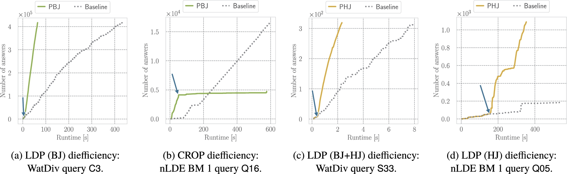
Next, we investigate the impact of the polymorphic join operators on the continuous production of answers by means of the diefficiency. To this end, we visualize the cumulative number of answers produced with respect to the query runtime for four example queries in Fig. 6. The first two queries (Fig. 6(a) and Fig. 6(b)) compare the baseline to the configuration with the PBJ enabled. For query C3 from the WatDiv benchmark and the LDP (BJ) planner, we can observe that after obtaining a few hundred tuples from the initial access operator of the query, the PBJ operators switch to the hash join strategy. Only the last PBJ in the query plan does not switch its strategy due to the large number of matching triples for the last triple pattern in the join order:
The second two plots (Fig. 6(c) and Fig. 6(d)) compare the baseline to the configuration with the PHJ enabled. While we can observe the potentially detrimental effect of the PBJ in the case that it switches its join strategy too early, the PHJ yields consistent improvements in diefficiency. As shown for example for query S33 in Fig. 6(c) and query Q05 in Fig. 6(d), the PHJ adapts its join strategy appropriately in both cases. The adaptivity substantially improves the diefficiency and reduces the total number of requests of the query plan execution. Due to the higher selectivity of the first join operator in the query plan for S33, the PHJ switches its join strategy rather quickly, while in Q05 the operator switches later during the execution as more tuples are produced by the preceding joins.
Fig. 7.
Scatter plots of the runtimes (log-log scale) for all planners with and without adaptive join operators. Value above the diagonal indicate performance degradation with adaptivity and values below performance improvement.
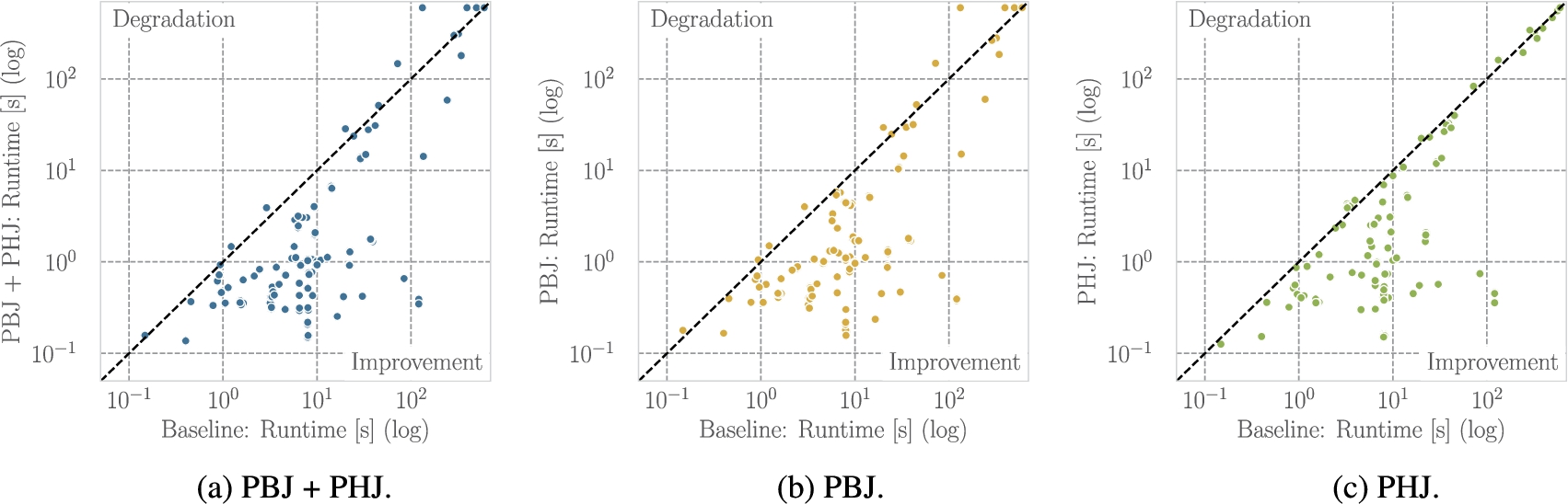
As a summary, we compare the runtimes of all planners for each query with and without adaptivity in Fig. 7. Each dot represents the runtimes of a query with and without adaptivity for a specific planner. Dots below the diagonal line represent an improvement in the execution performance (lower runtime is better). Overall, for the combination of PBJ and PHJ (Fig. 7(a)), we observe that, for the majority of queries, the polymorphic join operators allow for improving the robustness of query plan execution by adapting their join strategy. For just the PBJ (Fig. 7(b)), we observe a few queries where the performance substantially degrades while the majority yield a performance improvement. As expected, for the PHJ (Fig. 7(c)), we see that the runtime of the majority of queries improves. Just a few queries are slightly above the diagonal line which is likely to be attributed to runtime conditions. Combining the theoretical properties and the empirical evaluation of the PHJ, our findings show that the opportunity of improving the query execution efficiency with PHJ outweighs the potential risk of performance degradation. For the PBJ, we find that (with the current parameters) in many cases there is a higher risk of performance degradation. Therefore, future work should further investigate and improve the PBJ operator and its parameterization to reduce this risk.
7.Conclusion
In this work, we investigated different robust query processing techniques for Linked Data Fragments. In particular, we proposed two approaches to overcome the challenges of join cardinality estimation errors to devise efficient query planning and execution.
Our first approach, a cost- and robustness-based query plan optimizer (CROP), devises plans that are robust with respect to cardinality estimation errors. We propose a cost model to estimate the cost of query plans that combines local processing and network costs. We assess the robustness of a query plan using the cost ratio robustness measure, which compares the query plan’s best-case cost to its average-case cost (RQ 1). While the best-case cost assumes optimistic cardinality estimations, the average-case cost accounts for potential estimation errors by incorporating alternative, less optimistic cardinality estimations. Our query planner combines the cost model and robustness measure to devise efficient query plans. The results of our experimental study provide the following insights regarding RQ 2: (1) Including the robustness measure improves the query plan efficiency for queries with s-o and o-o joins. (2) In the case that the cheapest plan is not robust enough, an alternative robust plan that is not too expensive should be chosen. (3) CROP overall outperforms state of the art TPF clients.
In our second approach, we focus on query execution robustness by adapting the operators to estimation errors. To this end, we propose a new class of adaptive join operators that are able to switch their join strategy at runtime. We propose a Polymorphic Bind Join (PBJ) and a Polymorphic Hash Join (PHJ), which are able to switch their join strategy from a bind to hash join and vice versa. Our theoretical analysis proves the correctness of both operators under set semantics. In our empirical evaluation, we investigate the impact of PBJ and PHJ on the query execution efficiency for different planning approaches. The results show that especially the left-deep query planning approaches benefit from the adaptivity of the operators. In addition, we find that the gains in robustness during query execution depend on the operator and query characteristics. Specifically, the PHJ consistently enables more robust query execution, while the PBJ yields better results for the more selective queries in the WatDiv benchmark (RQ 3).
Concluding, we found that robust query processing approaches for Linked Data Fragments enable more efficient query execution. Robust query planning approaches help to devise efficient query plans that are less prone to potential cardinality estimation errors. Adaptive join operators can enhance the robustness during query execution by reducing the impact of sub-optimal query planning decisions. Future work may continue in both directions. Our query planning approach should be extended and evaluated for additional LDF interfaces. Moreover, existing clients for LDF interfaces, such as Comunica or smart-KG, could benefit from implementing the cost model and the robustness measure. In the area of adaptive join operators, future work should investigate alternative switch rules for the polymorphic join operators, e.g., by considering information from the query planner similar to [8] and [21]. In addition, other types of polymorphic join operators should be studied. For instance, operators that are able to switch their strategies several times. Lastly, the operators can be extended to further leverage the properties of the LDF interfaces, such as sorted tuples or the support of several bindings in the expressions.
Notes
5 We only consider binary join operators, resulting in a binary tree.
6 See for example [17], where the concept of polymorphism refers to adapting the block size according to the LDF interface while in this work it refers to adapting the join strategy.
7 In the pseudocode, we use the receive keyword to indicate asynchronicity: The operator determines whether the next tuple is available in the stream and if this is not the case, it continues its operation without executing the dependent steps.
8 We choose to describe the operator with the set O to provide a more intuitive description and proof of correctness.
14 Results are aggregated per query group in WatDiv.
15 Similar to Lines 10–15 in Algorithm 1 of [1].
References
[1] | M. Acosta and M. Vidal, Networks of linked data eddies: An adaptive web query processing engine for RDF data, in: The Semantic Web – ISWC 2015 – 14th International Semantic Web Conference, Bethlehem, PA, USA, October 11–15, 2015, Proceedings, Part I, M. Arenas, Ó. Corcho, E. Simperl, M. Strohmaier, M. d’Aquin, K. Srinivas, P. Groth, M. Dumontier, J. Heflin, K. Thirunarayan and S. Staab, eds, Lecture Notes in Computer Science, Vol. 9366: , Springer, (2015) , pp. 111–127. doi:10.1007/978-3-319-25007-6_7. |
[2] | M. Acosta, M. Vidal, T. Lampo, J. Castillo and E. Ruckhaus, ANAPSID: An adaptive query processing engine for SPARQL endpoints, in: The Semantic Web – ISWC 2011 – 10th International Semantic Web Conference, Bonn, Germany, October 23–27, 2011, Proceedings, Part I, L. Aroyo, C. Welty, H. Alani, J. Taylor, A. Bernstein, L. Kagal, N.F. Noy and E. Blomqvist, eds, Lecture Notes in Computer Science, Vol. 7031: , Springer, (2011) , pp. 18–34. doi:10.1007/978-3-642-25073-6_2. |
[3] | M. Acosta, M. Vidal and Y. Sure-Vetter, Diefficiency metrics: Measuring the continuous efficiency of query processing approaches, in: The Semantic Web – ISWC 2017 – 16th International Semantic Web Conference, Vienna, Austria, October 21–25, 2017, Proceedings, Part II, C. d’Amato, M. Fernández, V.A.M. Tamma, F. Lécué, P. Cudré-Mauroux, J.F. Sequeda, C. Lange and J. Heflin, eds, Lecture Notes in Computer Science, Vol. 10588: , Springer, (2017) , pp. 3–19. doi:10.1007/978-3-319-68204-4_1. |
[4] | G. Aluç, O. Hartig, M.T. Özsu and K. Daudjee, Diversified stress testing of RDF data management systems, in: The Semantic Web – ISWC 2014 – 13th International Semantic Web Conference, Riva del Garda, Italy, October 19–23, 2014. Proceedings, Part I, P. Mika, T. Tudorache, A. Bernstein, C. Welty, C.A. Knoblock, D. Vrandecic, P. Groth, N.F. Noy, K. Janowicz and C.A. Goble, eds, Lecture Notes in Computer Science, Vol. 8796: , Springer, (2014) , pp. 197–212. doi:10.1007/978-3-319-11964-9_13. |
[5] | C.B. Aranda, M. Arenas and Ó. Corcho, Semantics and optimization of the SPARQL 1.1 federation extension, in: The Semanic Web: Research and Applications – 8th Extended Semantic Web Conference, ESWC 2011, Heraklion, Crete, Greece, May 29 – June 2, 2011, Proceedings, Part II, G. Antoniou, M. Grobelnik, E.P.B. Simperl, B. Parsia, D. Plexousakis, P.D. Leenheer and J.Z. Pan, eds, Lecture Notes in Computer Science, Vol. 6644: , Springer, (2011) , pp. 1–15. doi:10.1007/978-3-642-21064-8_1. |
[6] | A. Azzam, J.D. Fernández, M. Acosta, M. Beno and A. Polleres, SMART-KG: Hybrid shipping for SPARQL querying on the web, in: WWW ’20: The Web Conference, 2020, Taipei, Taiwan, April 20–24, 2020, Y. Huang, I. King, T. Liu and M. van Steen, eds, ACM / IW3C2, (2020) , pp. 984–994. doi:10.1145/3366423.3380177. |
[7] | B. Babcock and S. Chaudhuri, Towards a robust query optimizer: A principled and practical approach, in: Proceedings of the ACM SIGMOD International Conference on Management of Data, Baltimore, Maryland, USA, June 14–16, 2005, F. Özcan, ed., ACM, (2005) , pp. 119–130. doi:10.1145/1066157.1066172. |
[8] | S. Babu, P. Bizarro and D.J. DeWitt, Proactive re-optimization, in: Proceedings of the ACM SIGMOD International Conference on Management of Data, Baltimore, Maryland, USA, June 14–16, 2005, F. Özcan, ed., ACM, (2005) , pp. 107–118. doi:10.1145/1066157.1066171. |
[9] | A. Charalambidis, A. Troumpoukis and S. Konstantopoulos, SemaGrow: Optimizing federated SPARQL queries, in: Proceedings of the 11th International Conference on Semantic Systems, SEMANTICS 2015, Vienna, Austria, September 15–17, 2015, A. Polleres, T. Pellegrini, S. Hellmann and J.X. Parreira, eds, ACM, (2015) , pp. 121–128. doi:10.1145/2814864.2814886. |
[10] | A. Deshpande, Z.G. Ives and V. Raman, Adaptive query processing, Found. Trends Databases 1: (1) ((2007) ), 1–140. doi:10.1561/1900000001. |
[11] | J.D. Fernández, M.A. Martínez-Prieto, C. Gutiérrez, A. Polleres and M. Arias, Binary RDF representation for publication and exchange (HDT), J. Web Semant. 19: ((2013) ), 22–41. doi:10.1016/j.websem.2013.01.002. |
[12] | O. Görlitz and S. Staab, SPLENDID: SPARQL endpoint federation exploiting VOID descriptions, in: Proceedings of the Second International Workshop on Consuming Linked Data (COLD2011), Bonn, Germany, October 23, 2011, O. Hartig, A. Harth and J.F. Sequeda, eds, CEUR Workshop Proceedings, Vol. 782: , CEUR-WS.org, (2011) , http://ceur-ws.org/Vol-782/GoerlitzAndStaab_COLD2011.pdf. |
[13] | A. Gounaris, N.W. Paton, A.A.A. Fernandes and R. Sakellariou, Adaptive query processing: A survey, in: Advances in Databases, 19th British National Conference on Databases, BNCOD 19, Sheffield, UK, July 17–19, 2002, Proceedings, B. Eaglestone, S. North and A. Poulovassilis, eds, Lecture Notes in Computer Science, Vol. 2405: , Springer, (2002) , pp. 11–25. doi:10.1007/3-540-45495-0_2. |
[14] | O. Hartig and C.B. Aranda, Bindings-restricted triple pattern fragments, in: On the Move to Meaningful Internet Systems: OTM 2016 Conferences – Confederated International Conferences: CoopIS, C&TC, and ODBASE 2016, Rhodes, Greece, October 24–28, 2016, Proceedings, C. Debruyne, H. Panetto, R. Meersman, T.S. Dillon, E. Kühn, D. O’Sullivan and C.A. Ardagna, eds, Lecture Notes in Computer Science, Vol. 10033: , (2016) , pp. 762–779. doi:10.1007/978-3-319-48472-3_48. |
[15] | O. Hartig, I. Letter and J. Pérez, A formal framework for comparing linked data fragments, in: The Semantic Web – ISWC 2017 – 16th International Semantic Web Conference, Vienna, Austria, October 21–25, 2017, Proceedings, Part I, C. d’Amato, M. Fernández, V.A.M. Tamma, F. Lécué, P. Cudré-Mauroux, J.F. Sequeda, C. Lange and J. Heflin, eds, Lecture Notes in Computer Science, Vol. 10587: , Springer, (2017) , pp. 364–382. doi:10.1007/978-3-319-68288-4_22. |
[16] | L. Heling and M. Acosta, Cost- and robustness-based query optimization for linked data fragments, in: The Semantic Web – ISWC 2020 – 19th International Semantic Web Conference, Athens, Greece, November 2–6, 2020, Proceedings, Part I, J.Z. Pan, V.A.M. Tamma, C. d’Amato, K. Janowicz, B. Fu, A. Polleres, O. Seneviratne and L. Kagal, eds, Lecture Notes in Computer Science, Vol. 12506: , Springer, (2020) , pp. 238–257. doi:10.1007/978-3-030-62419-4_14. |
[17] | L. Heling and M. Acosta, A framework for federated SPARQL query processing over heterogeneous linked data fragments, CoRR abs/2102.03269, 2021. https://arxiv.org/abs/2102.03269. |
[18] | L. Heling, M. Acosta, M. Maleshkova and Y. Sure-Vetter, Querying large knowledge graphs over triple pattern fragments: An empirical study, in: The Semantic Web – ISWC 2018 – 17th International Semantic Web Conference, Monterey, CA, USA, October 8–12, 2018, Proceedings, Part II, D. Vrandecic, K. Bontcheva, M.C. Suárez-Figueroa, V. Presutti, I. Celino, M. Sabou, L. Kaffee and E. Simperl, eds, Lecture Notes in Computer Science, Vol. 11137: , Springer, (2018) , pp. 86–102. doi:10.1007/978-3-030-00668-6_6. |
[19] | D. Kossmann and K. Stocker, Iterative dynamic programming: A new class of query optimization algorithms, ACM Trans. Database Syst. 25: (1) ((2000) ), 43–82. doi:10.1145/352958.352982. |
[20] | S.J. Lynden, I. Kojima, A. Matono and Y. Tanimura, ADERIS: An adaptive query processor for joining federated SPARQL endpoints, in: On the Move to Meaningful Internet Systems: OTM 2011 – Confederated International Conferences: CoopIS, DOA-SVI, and ODBASE 2011, Hersonissos, Crete, Greece, October 17–21, 2011, Proceedings, Part II, R. Meersman, T.S. Dillon, P. Herrero, A. Kumar, M. Reichert, L. Qing, B.C. Ooi, E. Damiani, D.C. Schmidt, J. White, M. Hauswirth, P. Hitzler and M.K. Mohania, eds, Lecture Notes in Computer Science, Vol. 7045: , Springer, (2011) , pp. 808–817. doi:10.1007/978-3-642-25106-1_28. |
[21] | V. Markl, V. Raman, D.E. Simmen, G.M. Lohman and H. Pirahesh, Robust query processing through progressive optimization, in: Proceedings of the ACM SIGMOD International Conference on Management of Data, Paris, France, June 13–18, 2004, G. Weikum, A.C. König and S. Deßloch, eds, ACM, (2004) , pp. 659–670. doi:10.1145/1007568.1007642. |
[22] | T. Minier, H. Skaf-Molli and P. Molli, SaGe: Web preemption for public SPARQL query services, in: The World Wide Web Conference, WWW 2019, San Francisco, CA, USA, May 13–17, 2019, L. Liu, R.W. White, A. Mantrach, F. Silvestri, J.J. McAuley, R. Baeza-Yates and L. Zia, eds, ACM, (2019) , pp. 1268–1278. doi:10.1145/3308558.3313652. |
[23] | G. Montoya, H. Skaf-Molli and K. Hose, The odyssey approach for optimizing federated SPARQL queries, in: The Semantic Web – ISWC 2017 – 16th International Semantic Web Conference, Vienna, Austria, October 21–25, 2017, Proceedings, Part I, C. d’Amato, M. Fernández, V.A.M. Tamma, F. Lécué, P. Cudré-Mauroux, J.F. Sequeda, C. Lange and J. Heflin, eds, Lecture Notes in Computer Science, Vol. 10587: , Springer, (2017) , pp. 471–489. doi:10.1007/978-3-319-68288-4_28. |
[24] | B. Quilitz and U. Leser, Querying distributed RDF data sources with SPARQL, in: The Semantic Web: Research and Applications, 5th European Semantic Web Conference, ESWC 2008, Tenerife, Canary Islands, Spain, June 1–5, 2008, Proceedings, S. Bechhofer, M. Hauswirth, J. Hoffmann and M. Koubarakis, eds, Lecture Notes in Computer Science, Vol. 5021: , Springer, (2008) , pp. 524–538. doi:10.1007/978-3-540-68234-9_39. |
[25] | M. Saleem, A. Potocki, T. Soru, O. Hartig and A.N. Ngomo, CostFed: Cost-based query optimization for SPARQL endpoint federation, in: Proceedings of the 14th International Conference on Semantic Systems, SEMANTICS 2018, Vienna, Austria, September 10–13, 2018, A. Fensel, V. de Boer, T. Pellegrini, E. Kiesling, B. Haslhofer, L. Hollink and A. Schindler, eds, Procedia Computer Science, Vol. 137: , Elsevier, (2018) , pp. 163–174. doi:10.1016/j.procs.2018.09.016. |
[26] | M. Schmidt, M. Meier and G. Lausen, Foundations of SPARQL query optimization, in: PDatabase Theory – ICDT 2010, 13th International Conference, Lausanne, Switzerland, March 23–25, 2010, Proceedings, L. Segoufin, ed., ACM International Conference Proceeding Series, ACM, (2010) , pp. 4–33. doi:10.1145/1804669.1804675. |
[27] | R. Taelman, J.V. Herwegen, M.V. Sande and R. Verborgh, Comunica: A modular SPARQL query engine for the web, in: The Semantic Web – ISWC 2018 – 17th International Semantic Web Conference, Monterey, CA, USA, October 8–12, 2018, Proceedings, Part II, D. Vrandecic, K. Bontcheva, M.C. Suárez-Figueroa, V. Presutti, I. Celino, M. Sabou, L. Kaffee and E. Simperl, eds, Lecture Notes in Computer Science, Vol. 11137: , Springer, (2018) , pp. 239–255. doi:10.1007/978-3-030-00668-6_15. |
[28] | R. Verborgh, M.V. Sande, O. Hartig, J.V. Herwegen, L.D. Vocht, B.D. Meester, G. Haesendonck and P. Colpaert, Triple pattern fragments: A low-cost knowledge graph interface for the web, J. Web Semant. 37–38: ((2016) ), 184–206. doi:10.1016/j.websem.2016.03.003. |
[29] | J.L. Wiener, H.A. Kuno and G. Graefe, Benchmarking query execution robustness, in: Performance Evaluation and Benchmarking, First TPC Technology Conference, TPCTC 2009, Lyon, France, August 24–28, 2009, Revised Selected Papers, R.O. Nambiar and M. Poess, eds, Lecture Notes in Computer Science, Vol. 5895: , Springer, (2009) , pp. 153–166. doi:10.1007/978-3-642-10424-4_12. |
[30] | F. Wolf, M. Brendle, N. May, P.R. Willems, K. Sattler and M. Grossniklaus, Robustness metrics for relational query execution plans, Proc. VLDB Endow. 11: (11) ((2018) ), 1360–1372, http://www.vldb.org/pvldb/vol11/p1360-wolf.pdf. doi:10.14778/3236187.3236191. |
[31] | E. Wössner, C. Qin, J. Fernández and M. Acosta, Triple pattern join cardinality estimations over HDT with enhanced metadata, in: Proceedings of the Posters and Demo Track of the 15th International Conference on Semantic Systems Co-Located with 15th International Conference on Semantic Systems (SEMANTiCS 2019), Karlsruhe, Germany, September 9th – to – 12th, 2019, M. Alam, R. Usbeck, T. Pellegrini, H. Sack and Y. Sure-Vetter, eds, CEUR Workshop Proceedings, Vol. 2451: , CEUR-WS.org, (2019) , http://ceur-ws.org/Vol-2451/paper-31.pdf. |
[32] | S. Yin, A. Hameurlain and F. Morvan, Robust query optimization methods with respect to estimation errors: A survey, SIGMOD Rec. 44: (3) ((2015) ), 25–36. doi:10.1145/2854006.2854012. |


