
Is the data normally distributed?
1Introduction
The normal distribution is the foundation of many statistical analysis techniques. These so called ‘parametric methods’ use the parameters of the distribution (mean, standard deviation) as part of the calculations. When data is analysed using parametric statistics, certain conditions should be met to apply those statistics correctly. One of these conditions is that data are normally distributed, and some suggest that this should be determined early in any analysis [1, 2]. But others suggest it is unnecessary [3], as normality is not an important assumption [4] and many parametric tests are ‘robust’ and can deal with non-normal data distributions [3]. Yet, readers of research papers seek assurances that the data analysis is appropriate [5].
In spite of authors discussing their need, Thode [6] described approximately 400 methods to test for normality. So, many options are available to researchers which range from informal plotting through to formal hypothesis testing which tests the null hypothesis of ‘the variable being examined follows a normal distribution’ [1]. So, a P value below a given significance level, suggests departure from normality.
Researchers need to be aware of these techniques, so that they can determine their analysis options, and to make sure the data contains no surprises. The purpose of this paper is to outline some of the techniques that can be used.
2Plotting data
Healy [4] suggested that looking at your data is the best way to determine non-normality. A researcher should visually inspect their data first, [1, 7] and not doing so is according to Tukey [8], inexcusable. Henderson [7] said that the first step in analysis was to screen the data for outliers. The box plot in Fig. 1 shows a distribution, with two ‘extreme’ high values. The researcher can determine if they are outliers or typos.
Next, the data should be plotted in a histogram [1, 7]. This ‘eye balling’ enables assessing whether the data approximates to a normal distribution, and if the data has a tail. Figure 2 displays several histograms of 90 90 test data scores. Selected parameters of the distributions are shown in Table 1. In Fig. 2, the distributions of the samples are different, Fig. A and B have much flatter distributions than C and D, which is largely down to the respective sample sizes. Larger samples will approximate more closely to a normal distribution. Kim [9] suggests that using the histogram of the distribution may be is best in a larger sample (n > 50). Certainly, the two distributions with smaller sample sizes in Fig. 1 (A & B) are flatter and lack the distinctive shape that is beginning to emerge in Figs. A and D.
Data distributions could also be examined using a graphic called a normal probability plot, sometimes know as a Q-Q probability plot. If the data approximates to a normal distribution, it should form a straight line along the upward diagonal [1, 9, 10]. Any departures from the line are evidence of a non-normal data distribution, for example Healy [4] stated that skewness can be seen if the data forms a curve. The normal probability plots for each of the samples are shown in Fig. 3. Each sample approximates quite well to the straight line. At either end of the four distributions, there is some departure from the diagonal. In each case it is not large, but it is most marked in the smaller samples (A & B). Figure 4 shows plots for positive and negative skewed distributions. Their departure from the diagonal is marked, and they are clearly non-normal.
3Summary statistics
Skewness is a measure of the asymmetry of the sample distribution [11, 12]. It is offered by many statistical packages and is also a function included in Excel [skew()]. So, it is readily accessible to researchers. For a true normal distribution the skewness parameter would be zero. A distribution is said to have a positive skew, when more data is in the right side of the distribution. A distribution is said to have a negative skew when most of the data values are on the left of the distribution. From the sample distributions in Fig. 1 and Table 1, A has a positive skew and B, C and D all have a negative skew. However, none of the values, exceed a value of±2, which is considered as the point where the distribution departs substantially from normality [9]. Another measure of departure from normality is a Z test as defined in Equation 1.
(1)
(2)
For this calculation the standard error of the skew is needed, the estimate [13] is given in Equation 2. As with any Z test the critical cut off at P < 0.05 is 1.96.
4Significance tests
Researchers can apply significance tests to determine if there the data depart from normality. Two popular tests are the Shapiro-Wilk test, and the Kolmogorov-Smirnoff test. The statistics for the six samples studied are in Table 2. The results for the first four (A, B, C & D) all recorded data above P > 0.05 and indicate normality, whereas for samples E and F, the low P values indicate that the data is not normally distributed. Sainani [1] regards using these tests as optional, and if used they should accompany graphical techniques. While the Shapiro-Wilk test is more powerful than the Kolmogorov-Smirnoff test [9], it is best used with samples of under 300 [9]. With samples larger than this, it is unreliable [9] as it emphasises unimportant deviations [1]. In contrast, important deviations may be disregarded in small samples [1].
Just because a variable is continuous (an interval or ratio scale) does not mean the data is normally distributed. This is especially true when dealing with small samples. Any data set should be examined for normality before applying a test for differences or associations. Many techniques are available to assess normality, and researchers are urged to use a variety of methods to assess their data. Frequently in physiotherapy research, relatively small sample sizes are used (n < 50). Examine your data and avoid surprises.
References
[1] | Sainani KL. Dealing with non-normal data. Physical Medicine and Rehabilitation (2012) ;4: :1001–5. |
[2] | Lacher DA. Sampling distribution of skewness and kurtosis. Clinical Chemistry (1989) ;35: :320. |
[3] | Norman G. Likert scales, levels of measurement and the ‘laws’ of statistics. Advances in Health Science Education (2010) ;15: :625–32. |
[4] | Healy MJ. Statistics from the inside. 12. non-normal data. Archives of Diseases in Childhood (1994) ;70: (2):158–63. |
[5] | Altman DG, Bland JM. Detecting skewness from summary information. BMJ (1996) ;313: :1200. |
[6] | Thode HJ. Testing for normality. New York: Marcel Dekker; (2002) . |
[7] | Henderson R. Testing experimental data for uniform normality. Clinica Chem Acta (2006) ;366: :112–29. |
[8] | Tukey JW. Explaratory data analysis. Reading MA: Addison-Wesley Publishing Company; (1977) . |
[9] | Kim HY. Statistical notes for clinical researchers: Assessing normal distribution (1). Restorative Dentistry and Endodontics (2013) ;38: :245–8. |
[10] | Ghasemi A, Zahediasl S. Normality tests for statistical analysis: A guide for non-statisticians. International Journal of Endocrinology and Metabolism (2012) ;10: :486–9. |
[11] | Ho D, Yu CC. Descriptive statistics for modern test score distributions: Skewness, kurtosis, discreetness, and celing effects. Educational and Psychological Measurement (2015) ;75: :365–88. |
[12] | Kim HY. Statistical notes for clinical researchers: Assessing normal distributions (2) using skewness and kurtosis. Restorative Dentistry and Endodontics (2013) ;38: :52–4. |
[13] | Tabachnick BG, Fidell LS. Using multivariate statistics. London: Allyn and Bacon (2001) . |
Figures and Tables
Fig.1
Distribution of 90/90 test results (n = 96).
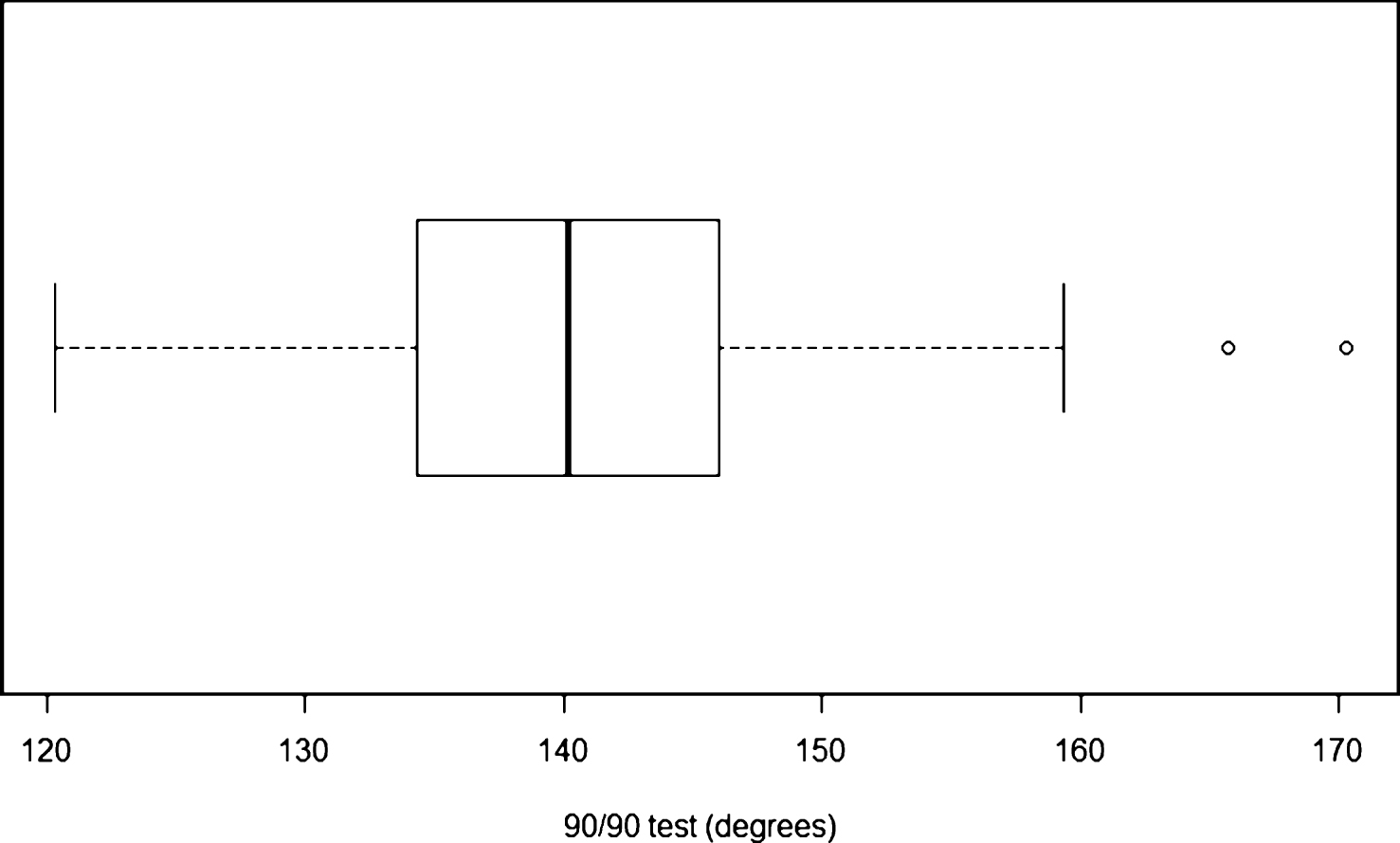
Fig.2
Histograms of four different samples of 90 90 test scores.
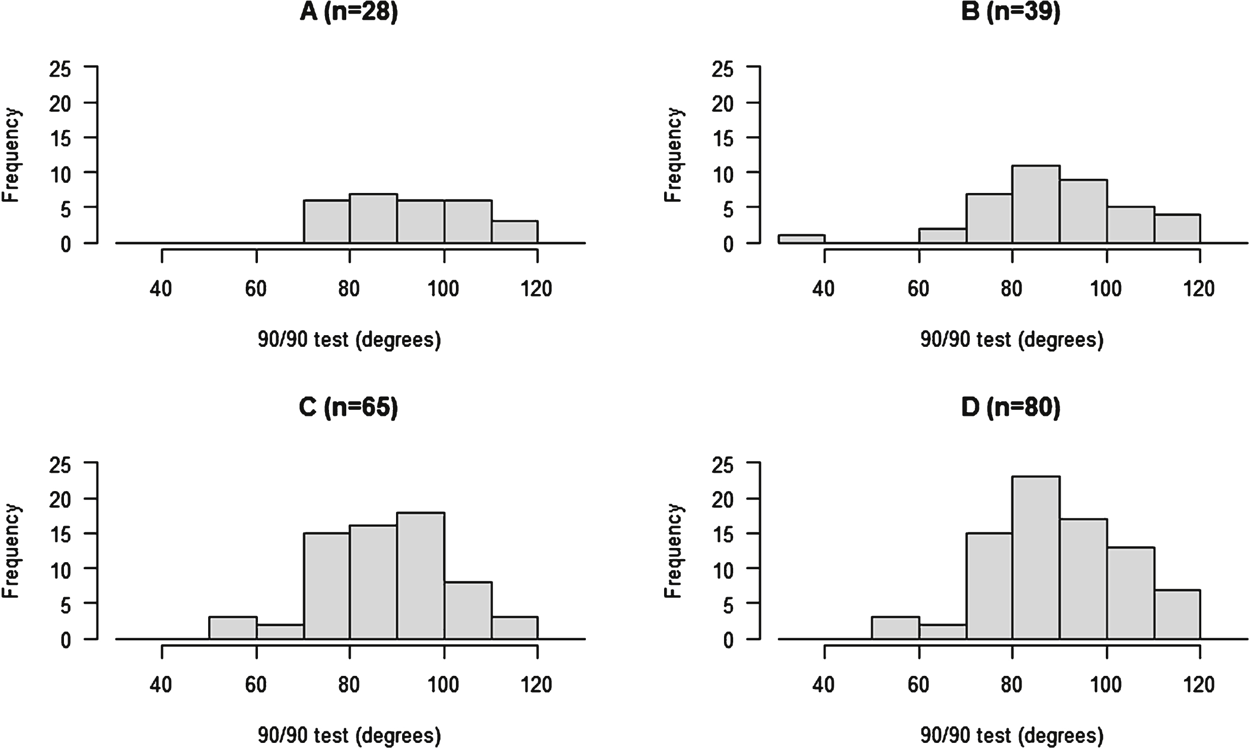
Fig.3
Normal probability plots of four different samples of 90 90 test scores.
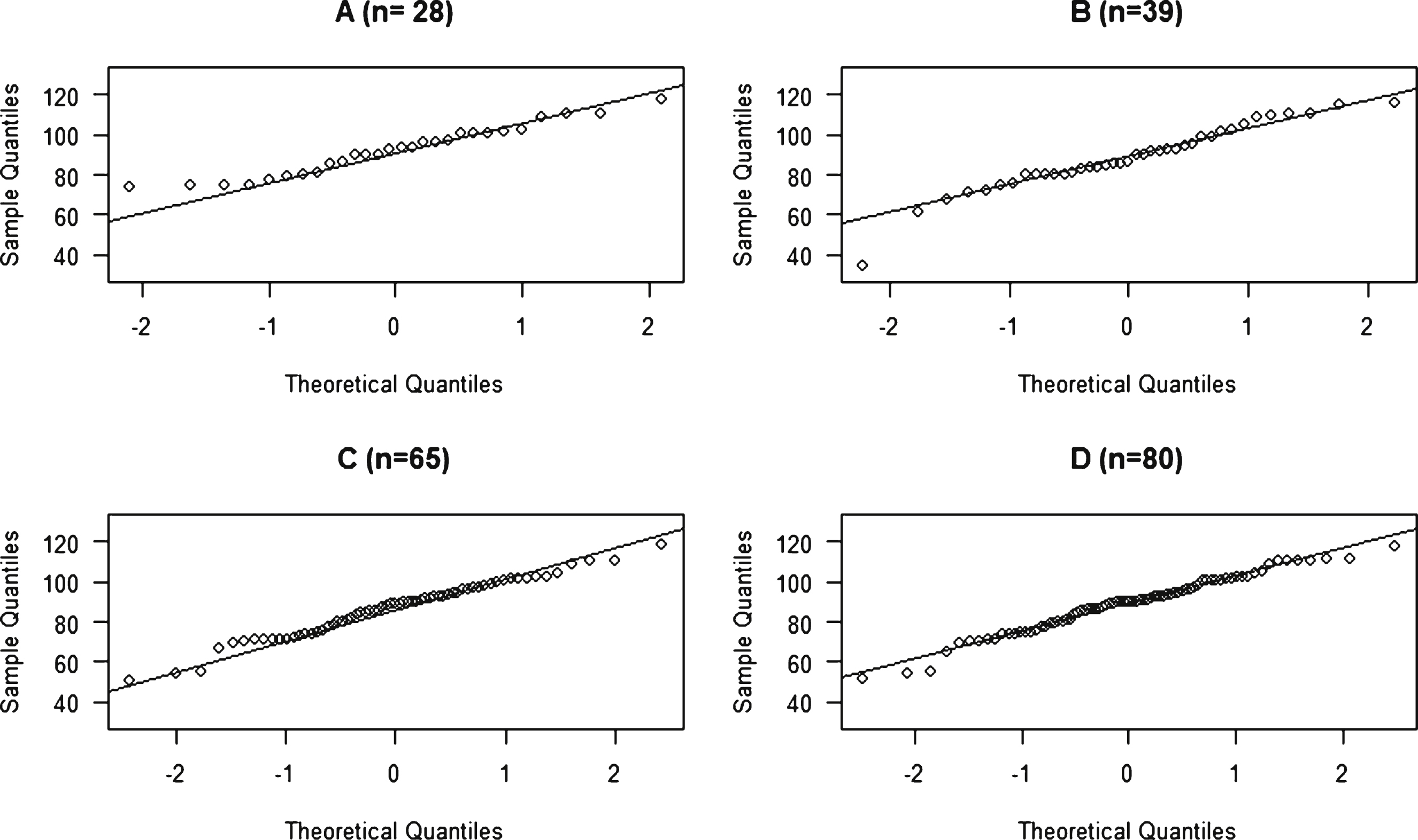
Fig.4
Normal probability plots of a positive(E) and a negative(F) skewed distribution.
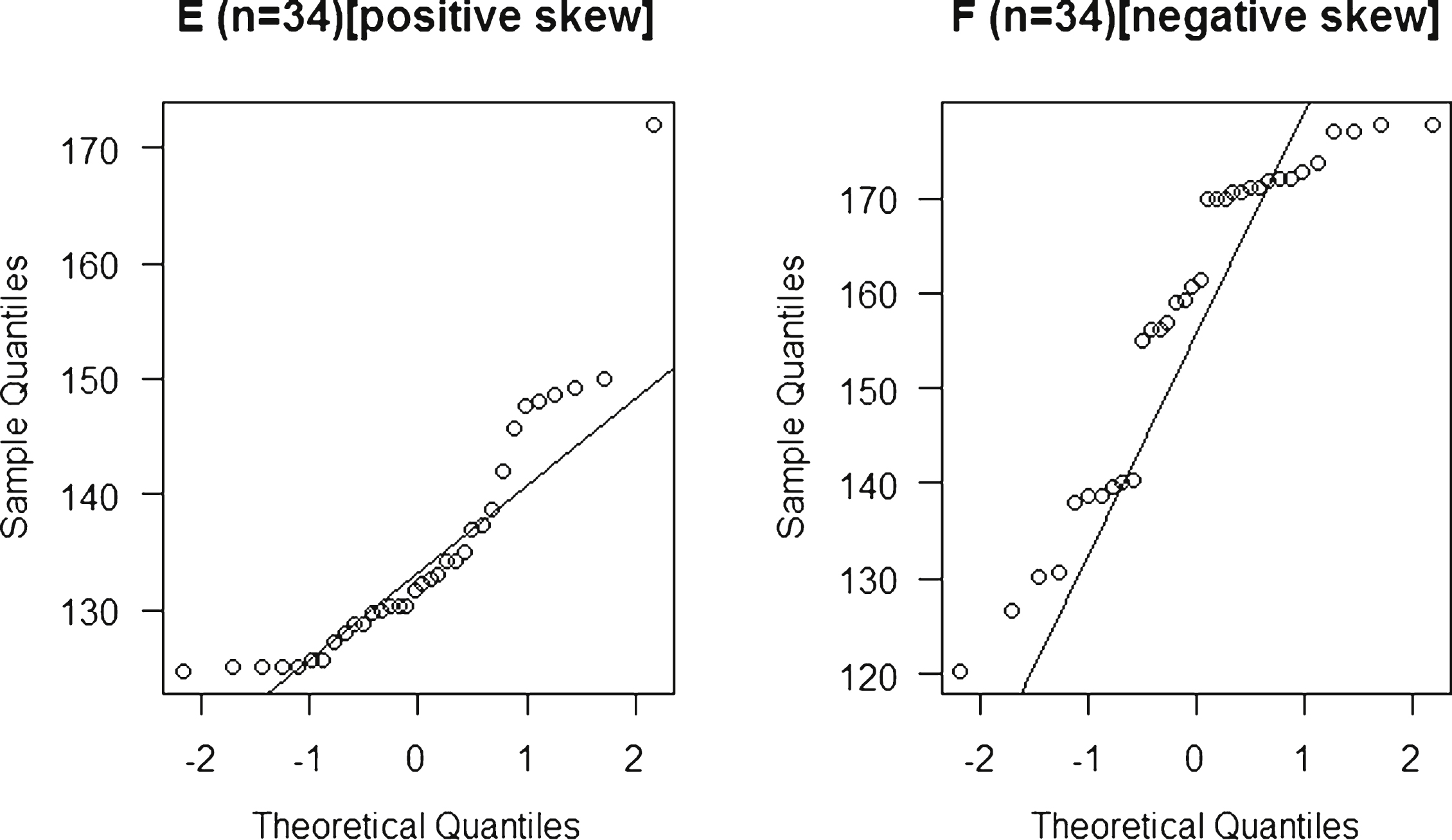
Table 1
Parameters of the four sample distributions
| n | Mean | SD | Skew | SEskew | Z | |
| A | 28 | 92.1 | 12.4 | 0.14 | 0.463 | 0.302 |
| B | 39 | 88.3 | 16.2 | –0.71 | 0.392 | –1.810 |
| C | 65 | 86.7 | 13.9 | –0.33 | 0.304 | –1.086 |
| D | 80 | 88.9 | 13.8 | –0.39 | 0.274 | –1.424 |
Table 2
Shapiro-Wilk tests for normality
| n | w | P | |
| A | 28 | 0.959 | 0.33 |
| B | 39 | 0.946 | 0.06 |
| C | 65 | 0.981 | 0.39 |
| D | 80 | 0.978 | 0.19 |
| E | 34 | 0.832 | 0.001 |
| F | 34 | 0.877 | 0.001 |


