
Inferences for generalized Topp-Leone distribution under dual generalized order statistics with applications to Engineering and COVID-19 data
Abstract
This article accentuates the estimation of a two-parameter generalized Topp-Leone distribution using dual generalized order statistics (dgos). In the part of estimation, we obtain maximum likelihood (ML) estimates and approximate confidence intervals of the model parameters using dgos, in particular, based on order statistics and lower record values. The Bayes estimate is derived with respect to a squared error loss function using gamma priors. The highest posterior density credible interval is computed based on the MH algorithm. Furthermore, the explicit expressions for single and product moments of dgos from this distribution are also derived. Based on order statistics and lower records, a simulation study is carried out to check the efficiency of these estimators. Two real life data sets, one is for order statistics and another is for lower record values have been analyzed to demonstrate how the proposed methods may work in practice.
1.Introduction
Shekhawat and Sharma (2020) introduced a new extension of Topp-Leone (TL) distribution on the unit interval by adding a skewness parameter in the TL distribution using the power transformation called the generalized Topp-Leone (GTL) distribution. The probability density Eq. (1) of GTL distribution is given by
(1)
and the corresponding cumulative distribution Eq. (2) and hazard function are given by
(2)
It can be seen that
(3)
Topp-Lone distribution is a member of GTL distribution if
Bounded distributions are increasingly gaining grounds in literature owing to their significance in several areas like psychology, economics, biology, engineering and many others. For instance, in psychology, proportions and percentages play a vital role in evaluating the probability of judgments (Smithson & Shou, 2017). Similarly in economics, one may come across several instances where data are bound on the unit interval. For example, proportion of income spent on non-durable consumption, pension plan participation rates, market shares, fractional repayment on debts and capital structures (Ghosh et al., 2019; Papke & Wooldridge, 1996; Smithson & Shou, 2017). Besides, for measuring reliability, it is imperative to have models defined on the unit interval in order to have plausible results (Genç, 2013).
Distributions based on unit interval are known to have desirable failure (hazard) rate characteristics such as increasing, decreasing and bathtub shapes. However, one may encounter situations where only increasing and bathtub failure rates are used or observed. These failure rate characteristics are vital when modeling datasets. For instance, Rajarshi and Rajarshi (1998), and Lawless (2003) in their studies observed that distributions with bathtub hazard rates are needed to model lifetime of electronic, electrochemical and mechanical products; while Lai (2013) observed that the optimum number of minimal repairs for systems have increasing failure rates. Also, it has been observed that during clinical development drugs have increasing failure rate (see Woosley and Cossman (2007)).
The concept of generalized order statistics (gos) has held the attention of statisticians for a long time. It was first proposed by Kamps (1995) and includes ordered random variables arranged in increasing order of magnitude such as order statistics, sequential order statistics, progressive type II censored order statistics, records and Pfeifers records. However, the ordered random variables which are arranged in decreasing order of magnitude can not be studied in this framework. Owing to this, statisticians felt the need for the ordered random variables which can also be arranged in decreasing order of magnitude. For example, the life length of an electric bulb arranged from highest to lowest. The study of distributional properties of such random variables by using the inverse image of gos is popularly known as dual generalized order statistics. Pawlas and Szynal (2001) first proposed the concept of dual generalized order statistics (dgos) wherein the order random variables can be studied in both increasing and decreasing order of magnitude. This concept was further studied in a systematic manner by Burkschat et al. (2003). Dual gos includes order statistics (reversed ordered order statistics), lower k-records and lower Pfeifer records. For better understanding, dgos can be used when
In the last two decades or so, several studies have been carried out on the statistical properties of continuous distributions based on dgos. In this regard, readers may refer to the works of Pawlas and Szynal (2001), Ahsanullah (2004, 2005), Mbah and Ahsanullah (2007), Anwar and Athar (2008), Barakat and El-Adll (2009), Khan et al. (2010), Khan and Kumar (2010, 2011), Jaheen and Al Harbi (2011), Athar and Faizan (2011), Kumar (2013a, b), Khan and Khan (2015), Kumar (2016), Li (2016), Kumar and Dey (2017), Khan and Iqrar (2019), Kumar et al. (2020) among others.
However, to the best of our knowledge, there are no reports on GTL distribution based on dgos. The motivation of the paper is two fold: first is to derive the explicit expressions for the single and the product moments based on dgos of GTL distribution. Second is to estimate the parameters of the model from both frequentist and Bayesian view points based on order statistics and lower record values.
The paper is organized as follows. In Section 2, we present preliminaries of dgos. In Section 3, we present explicit expressions for the single moments and product moments of order statistics of dgos of GTL distribution. In the same Section, we reported the mean and variances of order statistics and lower record values. Two methods of estimation namely, maximum likelihood method of estimation and Bayesian method of estimation are discussed in Section 4. To obtain the Bayes estimates, independent gamma priors of the unknown model parameters are used under squared error loss (SEL) function. In Section 5, simluation study is carried out to evaluate the performance of the ML and the Bayes estimates based on root mean squared error (RMSE) and relative absolute bias (RAB). In addition, average length (AL) and coverage percentages (CPs) for the 95% approximate confidence interval (ACI) and highest posterior density (HPD) credible intervals of the parameters under order statistics and lower record values is provided in the same Section. We illustrate the methodology developed in this manuscript and the usefulness of the GTL distribution based on two real-life data sets, one is for order statistics and another is for lower record values in Section 6. Finally, concluding remarks are provided in Section 7.
Some lemmas useful for the derivation of the explicit expressions are provided in APPENDIX. The lemmas make use of the Gauss hypergeometric function and Kampé de Feriet’s Function defined by
and
where
2.Dual generalized order statistics and preliminaries
The random variables
for
(4)
for
It follows also that the joint pdf of the
(5)
for
3.Relations for moments of the dgos from GTL distribution
In this section, we derive explicit expressions and recurrence relations for single and product moments of dgos given a random sample
3.1Relations for single moments of dgos
Here, first we present the explicit expressions and recurrence relations for rth dgos,
Theorem 1. For
(6)
where
Proof From Eq. (4), we get
The result follows by using Lemma 1. The proof is complete.
Corollary 1. For
(7)
where
Remark 1. Setting
That is
(8)
Remark 2. Putting
(9)
as obtained by Zghoul (2011) for
Theorem 2 establishes a recurrence relation for single moments
Theorem 2. For
(10)
Throughout, we follow the conventions that
Proof From Eqs (3) and (4), we have
Upon integrating by parts by treating
Corollary 2. For the GTL distribution given in Eq. (1)
Remark 3. Setting
Replacing
which verify the result of Zghoul (2010) for
Remark 4. Setting
and hence for lower records
as obtained by Zghoul (2011) for
3.2Relations for product moments of dgos
Here, first we present the explicit expressions and recurrence relations for rth and sth dgos,
Theorem 3. For
(11)
where
Proof From Eq. (5), we have
The result follows by using Lemma 2. The proof is complete.
Corollary 3. For
(12)
Remark 5. If
Remark 6. If
Theorem 4. For
(13)
Proof From Eqs (3) and (5), we have
Integrating by parts and treating
Remark 7. Setting
Which verifies the result of Kumar (2012) for
Remark 8. For
and hence for lower records
4.Estimation based on dgos
4.1Maximum likelihood estimation
Let
(14)
The natural logarithm of the likelihood function
(15)
By differentiating Eq. (15) partially with respect
and
The maximum likelihood estimator (MLE) of
(16)
where
The MLE of
(17)
where
To construct the
Practically, by dropping the expectation operator
(18)
From Eq. (18), the Fisher’s elements will be
and
Under some regularity conditions, the asymptotic normality of MLEs
where
4.2Bayesian estimation
In this subsection, we focus on obtaining the Bayes estimates of the unknown model parameters
(19)
Now, we can write the joint posterior distribution of
(20)
where
(21)
From Eq. (18) we can observe that it is not possible to obtain the Bayes estimators of
(22)
and
(23)
It is observed that the conditional posterior distributions of the unknown parameters
Step 5:
Step 1: Set an initial values
Step 2: Set
Step 3: Generate
(a) Generate
(b) Obtain
(c) Generate
(d) If
(e) If
Step 4: Set
Step 5: Redo steps 3–4 for
To construct the HPD credible intervals of
where
Here
5.Monte carlo simulation
In this section, a Monte Carlo simulation is conducted to examine and compare the performance of the proposed maximum likelihood and Bayes estimators of the unknown parameters
Step 7:
Step 1: Set two arbitrarily true values of
Step 2: Set hyper-parameters values of
Step 3: For
Step 4: Two special cases of dgos are considered, the first is the order statistics (OS) by taking
Step 5: Using Newton-Raphson iterative method, the MLEs
Step 6: Using Metropolis-Hastings within Gibbs algorithm described in Subsection 4.2, the MCMC Bayes estimates
Step 7: Repeat Steps 3–6 for 5,000 times and obtain the average estimates (AEs) for any parameteric function of
where
Extensive computations were performed using
Table 1
The AEs of
| ( |
| MLE | BE | ||
|---|---|---|---|---|---|
| OS | LR | OS | LR | ||
| (0.1, 0.5) | 20 | 0.3965 | 0.0946 | 0.0801 | 0.4120 |
| (2.1899, 3.6538) | (0.0239, 0.0538) | (0.0240, 0.2050) | (0.3296, 3.1202) | ||
| 40 | 0.2758 | 0.0972 | 0.0908 | 0.4856 | |
| (1.8928, 2.2698) | (0.0172, 0.0283) | (0.0143, 0.1181) | (0.4037, 3.8564) | ||
| 60 | 0.1747 | 0.0984 | 0.0896 | 0.5699 | |
| (1.1252, 1.1715) | (0.0127, 0.0156) | (0.0142, 0.1182) | (0.4838, 4.6988) | ||
| 80 | 0.1311 | 0.0987 | 0.1009 | 0.6847 | |
| (0.4632, 0.6936) | (0.0115, 0.0129) | (0.0101, 0.0808) | (0.6045, 5.8472) | ||
| 100 | 0.1171 | 0.0990 | 0.1047 | 0.7715 | |
| (0.1680, 0.5109) | (0.0104, 0.0105) | (0.0099, 0.0818) | (0.7032, 6.7148) | ||
| (0.2, 0.7) | 20 | 0.8413 | 0.1884 | 0.1924 | 0.5264 |
| (7.9099, 3.8938) | (0.0511, 0.0582) | (0.0357, 0.1524) | (0.3347, 1.6321) | ||
| 40 | 0.4543 | 0.1950 | 0.1962 | 0.5160 | |
| (3.5710, 1.8081) | (0.0333, 0.0252) | (0.0213, 0.0863) | (0.3332, 1.5801) | ||
| 60 | 0.3219 | 0.1970 | 0.2020 | 0.6019 | |
| (1.8096, 1.0412) | (0.0256, 0.0151) | (0.0224, 0.0847) | (0.4384, 2.0093) | ||
| 80 | 0.2344 | 0.1973 | 0.1950 | 0.6485 | |
| (0.6286, 0.5575) | (0.0243, 0.0136) | (0.0157, 0.0645) | (0.4655, 2.2424) | ||
| 100 | 0.2243 | 0.1981 | 0.1930 | 0.7917 | |
| (0.2461, 0.4669) | (0.0200, 0.0093) | (0.0141, 0.0565) | (0.6047, 2.9584) | ||
Table 2
The AEs of
| ( |
| MLE | BE | ||
|---|---|---|---|---|---|
| OS | LR | OS | LR | ||
| (0.1, 0.5) | 20 | 17.438 | 0.5045 | 0.5188 | 0.6678 |
| (87.216, 34.331) | (0.0201, 0.0090) | (0.0355, 0.0593) | (0.1769, 0.3357) | ||
| 40 | 3.1199 | 0.5024 | 0.5112 | 0.6333 | |
| (32.639, 5.6498) | (0.0148, 0.0049) | (0.0209, 0.0327) | (0.1413, 0.2665) | ||
| 60 | 1.0034 | 0.5014 | 0.4883 | 0.5382 | |
| (3.6558, 1.3772) | (0.0112, 0.0028) | (0.0190, 0.0314) | (0.0481, 0.0771) | ||
| 80 | 0.8228 | 0.5011 | 0.4887 | 0.5729 | |
| (1.8427, 0.9821) | (0.0102, 0.0023) | (0.0176, 0.0282) | (0.0846, 0.1458) | ||
| 100 | 0.7161 | 0.5009 | 0.5070 | 0.5852 | |
| (1.1628, 0.7523) | (0.0089, 0.0018) | (0.0156, 0.0249) | (0.0998, 0.1713) | ||
| (0.2, 0.7) | 20 | 32.329 | 0.7100 | 0.5882 | 0.8123 |
| (128.72, 45.638) | (0.0438, 0.0142) | (0.1160, 0.1597) | (0.1300, 0.1633) | ||
| 40 | 5.5303 | 0.7045 | 0.7056 | 0.8130 | |
| (36.371, 7.2950) | (0.0295, 0.0064) | (0.0185, 0.0213) | (0.1307, 0.1614) | ||
| 60 | 2.0287 | 0.7027 | 0.7074 | 0.6988 | |
| (14.341, 2.2711) | (0.0228, 0.0038) | (0.0178, 0.0205) | (0.0421, 0.0559) | ||
| 80 | 1.2408 | 0.7024 | 0.7008 | 0.7680 | |
| (2.6203, 1.1009) | (0.0216, 0.0035) | (0.0103, 0.0124) | (0.0731, 0.0972) | ||
| 100 | 1.0462 | 0.7016 | 0.7080 | 0.7540 | |
| (1.9061, 0.8135) | (0.0177, 0.0023) | (0.0160, 0.0175) | (0.0593, 0.0772) | ||
Table 3
The ALs of
| ( |
|
|
| ||||||
|---|---|---|---|---|---|---|---|---|---|
| ACI | HPD | ACI | HPD | ||||||
| OS | LR | OS | LR | OS | LR | OS | LR | ||
| (0.1, 0.5) | 20 | 283.90 | 0.4422 | 0.1054 | 0.1875 | 3.9013 | 0.0819 | 0.0466 | 0.3047 |
| (0.8678) | (0.9995) | (0.9900) | (0.9980) | (0.7652) | (0.9490) | (0.9766) | (0.9925) | ||
| 40 | 31.758 | 0.3114 | 0.0636 | 0.1384 | 1.9543 | 0.0598 | 0.0424 | 0.3484 | |
| (0.8930) | (0.9995) | (0.9720) | (0.9731) | (0.8334) | (0.9728) | (0.9660) | (0.9525) | ||
| 60 | 5.1739 | 0.2537 | 0.0517 | 0.0887 | 0.8119 | 0.0495 | 0.0370 | 0.4053 | |
| (0.9080) | (0.9997) | (0.9762) | (0.9799) | (0.8658) | (0.9848) | (0.9754) | (0.9997) | ||
| 80 | 2.8548 | 0.2196 | 0.0576 | 0.1306 | 0.4560 | 0.0431 | 0.0388 | 0.4801 | |
| (0.9178) | (0.9998) | (0.9880) | (0.9535) | (0.8778) | (0.9874) | (0.9849) | (0.9877) | ||
| 100 | 2.0738 | 0.1963 | 0.0492 | 0.1464 | 0.2787 | 0.0387 | 0.0334 | 0.6752 | |
| (0.9236) | (0.9999) | (0.9555) | (0.9830) | (0.8914) | (0.9898) | (0.9798) | (0.9967) | ||
| (0.2, 0.7) | 20 | 581.67 | 0.6201 | 0.1204 | 0.2123 | 9.0819 | 0.1630 | 0.1081 | 0.2381 |
| (0.8724) | (0.9990) | (0.9696) | (0.9760) | (0.7784) | (0.9480) | (0.9633) | (0.9958) | ||
| 40 | 66.834 | 0.4397 | 0.0714 | 0.1812 | 3.1801 | 0.1200 | 0.0754 | 0.3243 | |
| (0.8978) | (0.9998) | (0.9692) | (0.9660) | (0.8328) | (0.9772) | (0.9923) | (0.9887) | ||
| 60 | 16.072 | 0.3557 | 0.0634 | 0.1192 | 1.5496 | 0.0990 | 0.0896 | 0.5180 | |
| (0.9018) | (0.9998) | (0.9690) | (0.9652) | (0.8660) | (0.9860) | (0.9858) | (0.9922) | ||
| 80 | 4.8497 | 0.3078 | 0.0355 | 0.0903 | 0.5831 | 0.0861 | 0.0545 | 0.4193 | |
| (0.9172) | (0.9946) | (0.9595) | (0.9605) | (0.8822) | (0.9874) | (0.9823) | (0.9932) | ||
| 100 | 3.2833 | 0.2750 | 0.0496 | 0.0848 | 0.5018 | 0.0774 | 0.0469 | 0.4310 | |
| (0.9192) | (0.9914) | (0.9727) | (0.9649) | (0.8932) | (0.9914) | (0.9700) | (0.9958) | ||
Table 4
Lower record data from data 1
| 0.083 | 0.025 | 0.023 | 0.017 | 0.015 | 0.008 | 0.007 | 0.005 | 0.001 |
From Tables 1–3, we are able to make the following observations. The performances of the proposed estimates of
Also, the ALs of ACI/HPD credible intervals narrow down as
Further, the RMSEs and RABs associated with the BEs of
For interval estimates, the 95% HPD credible intervals are better than ACIs in respect of their ALs and CPs. Moreover, the ACIs of
6.Real-life data analysis
In this section, we analyze two real data sets to illustrate our established results. The first one based on lower record (LR) and the second one based on order statistics (OS). It is known that OR and LR can be obtained from the dgos as a special case, therefore, the estimators and confidence intervals of the GTL distribution based on LR and OS can be obtained directly from Section 4.
Example I: Analysis of Boeing 720 jet airplanes based on LR
The first data set consists of number of successive failure for the air conditioning system reported of each member in a fleet of 13 Boeing 720 jet airplanes studied by Tahir et al. (2015). Since the maximum number of successive failure is 603, the original data were transformed to be in the interval
Table 5
The MLEs, Bayes estimates, the corresponding SE (within parentheses) and the confidence/credible interval estimates based on LR data
| Parameter | MLE | Bayes estimates |
|---|---|---|
|
| 331.09 (177.45) | 330.629 (9.876) |
| (0.000, 447.40) | (310.95, 349.74) | |
|
| 0.0259 (0.0508) | 0.0256 (0.0034) |
| (0.000, 0.1493) | (0.0189, 0.0325) |
Table 6
Recovery rate of COVID-19 in Spain
| 0.667 | 0.500 | 0.490 | 0.429 | 0.750 | 0.653 | 0.516 | 0.789 | 0.769 | 0.687 |
| 0.520 | 0.725 | 0.638 | 0.608 | 0.659 | 0.629 | 0.571 | 0.592 | 0.606 | 0.592 |
| 0.592 | 0.559 | 0.595 | 0.616 | 0.646 | 0.672 | 0.684 | 0.685 | 0.695 | 0.707 |
| 0.721 | 0.732 | 0.741 | 0.751 | 0.752 | 0.755 | 0.764 | 0.771 | 0.776 | 0.781 |
| 0.784 | 0.785 | 0.787 | 0.790 | 0.796 | 0.793 | 0.791 | 0.796 | 0.797 | 0.798 |
| 0.801 | 0.804 | 0.829 | 0.832 | 0.835 | 0.837 | 0.839 | 0.846 | 0.849 | 0.852 |
| 0.854 | 0.855 | 0.856 | 0.858 | 0.860 | 0.863 |
Figure 1.
Estimated SF and P-P plots for real data 1.
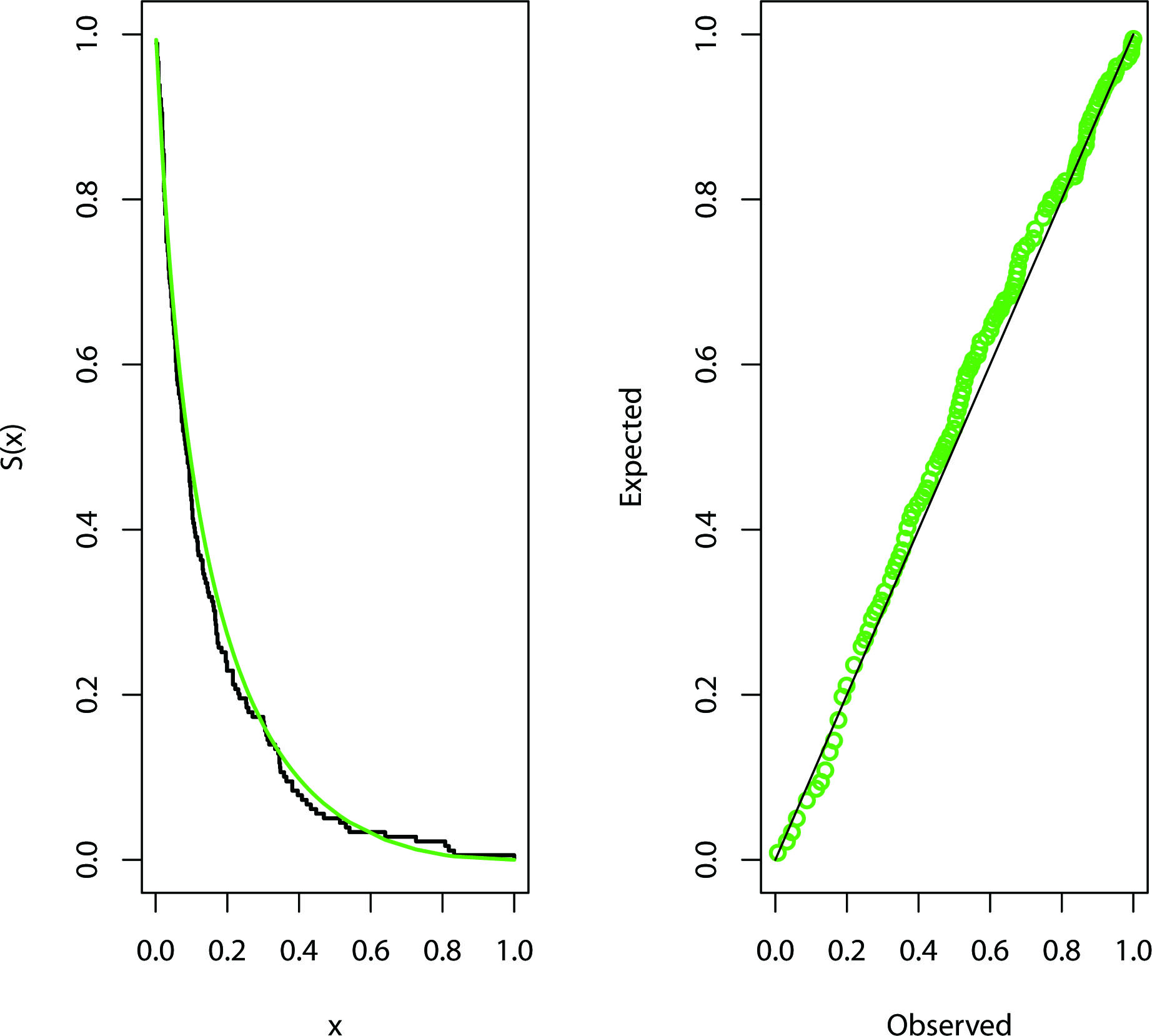
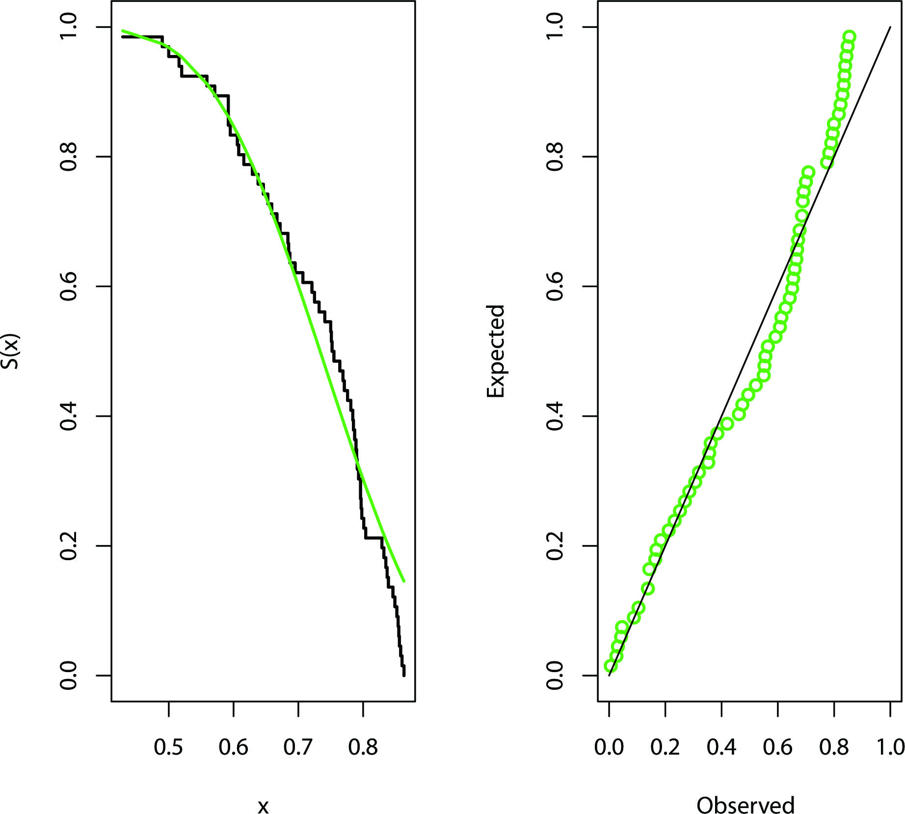
Example II: Analysis of recovery rate of COVID-19 in Spain based on OS
The second data set presents the daily recovery rate of COVID-19 in Spain from March 3 to May 7. The data consists of 66 daily recovery rate and available in https://www.worldometers.info/coronavirus/country/spain/. The data set is presented in Table 6. Since the data consists of the recovery rates of COVID-19 in Spain, which is a unit interval data, one of the choices to model this data set is the beta distribution. It is not easy to analyze the beta distribution under dgos because its cdf contains an incomplete beta function. In this case, the GTL distribution can be used as a good model with flexible pdf and cdf to analyze this data set as it is measured in the unit interval (0, 1). We first check whether the GTL distribution can be model to these data set. The Kolmogorov-Smirnov distance and the corresponding
Table 7
The MLEs, Bayes estimates, the corresponding SE (within parentheses) and the confidence/ credible interval estimates based OS data
| Parameter | MLE | Bayes estimates |
|---|---|---|
|
| 24557.3 (164118.8) | 24303.47 (493.501) |
| (0.000, 346230.21) | (23364.4, 25280.7) | |
|
| 0.01720 (0.0577) | 0.01721 (0.00073) |
| (0.000, 0.1303) | (0.01577, 0.01866) |
Figure 2.
Estimated SF and P-P plots for real data 2.
7.Conclusion
In this paper, first we have obtained the explicit expression for the single and product moments of dgos from GTL distribution. The results obtained in this paper are more generalized in the sense that it includes the moment of order statistics and lower records from GTL distribution. Further, ML and Bayes methods of estimation are used for estimation of the parameters of the GTL distribution based on order statistics and lower record values. A simulation study is carried out to compare the proposed estimators in terms of RMSE and RAB. In addition, ACIs and HPD credible intervals are compared in terms of their AL and CPs. From simulation and real data analysis, we observe that Bayesian approach is quite satisfactory as compared to non-Bayesian procedure for both OS and LR values. Although many properties of GTL distribution have been discussed recently, it seems that BLUEs/BLUPS of the parameters and prediction of future observations based on ordered data for this distribution have not been investigated yet. The work is in progress and it will be reported later.
Acknowledgments
The authors are grateful for the comments and suggestions by the referees and the associate editor. Their comments and suggestions have greatly improved the article.
References
[1] | Ahsanullah, M. ((2004) ). A characterization of the uniform distribution by dual generalized order statistics. Communications in Statistics-Theory and Methods, 33: , 2921-2928. |
[2] | Ahsanullah, M. ((2005) ). On lower generalized order statistics and a characterization of power function distribution. Statistical Methods, 7: , 16-28. |
[3] | Arnold, B. C., & Press, S. J. ((1983) ). Bayesian inference for Pareto populations. Journal of Econometrics, 21: , 287-306. |
[4] | Barakat, H. M., & El-Adll, M. E. ((2009) ). Asymptotic theory of extreme dual generalized order statistics. Stat Probabil Lett, 79: , 1252-1259. |
[5] | Burkschat, M., Cramer, E., & Kamps, U. ((2003) ). Dual generalized order statistics. Metron LXI, 13-26. |
[6] | Chen, M. H., & Shao, Q. M. ((1999) ). Monte Carlo estimation of Bayesian credible and HPD intervals. Journal of Computational and Graphical Statistics, 8: , 69-92. |
[7] | Cohen, A. C. ((1965) ). Maximum likelihood estimation in the Weibull distribution based on complete and censored samples. Technometrics, 5: , 579-588. |
[8] | Dey, S., Ali, S., Park, C. ((2015) ). Weighted exponential distribution: Properties and different methods of estimation. J Stat Comput Simul, 85: , 3641-3661. |
[9] | Dey, S., Dey, T., Ali, S., & Mulekar, M. S. ((2016) a). Two-parameter Maxwell distribution: Properties and different methods of estimation. J Stat Theory Prac, 10: , 291-310. |
[10] | Dey, S., Singh, S., & Tripathi, Y. M. ((2016) b). Estimation and prediction for a progressively censored generalized inverted exponential distribution. Stat Methodol, 32: , 185-202. |
[11] | Genç, A. I. ((2013) ). Estimation of P(X>Y) with Topp–Leone distribution. J Stat Comput Simul, 83: , 326-339. |
[12] | Ghosh, I., Dey, S., & Kumar, D. ((2019) ). Bounded M-O extended exponential distribution with applications. Stochastics and Quality Control, 34: , 35-51. |
[13] | Henningsen, A., & Toomet, O. ((2011) ). ‘MaxLik’: A package for maximum likelihood estimation in R. Computational Statistics, 26: , 443-458. |
[14] | Jaheen, Z. F., & Al Harbi, M. M. ((2011) ). Bayesian estimation based on dual generalized order statistics from the exponentiated Weibull model. J Stat Theory Appl, 10: , 591-602. |
[15] | Kamps, U. ((1995) ). A concept of generalized order statistics. B.G. Teubner Stuttgart. |
[16] | Khan, R. U., Anwar, Z., & Athar, H. ((2008) ). Recurrence relations for single and product moments of dual generalized order from exponentiatedWeibull distribution. Aligarh J Statist, 28: , 37-45. |
[17] | Khan, R. U., & Kumar, D. ((2010) ). On moments of generalized order statistics fromexponentiated Pareto distribution and its characterization. Applied Mathematical Sciences (Ruse), 4: , 2711-2722. |
[18] | Khan, R. U., & Kumar, D. ((2011) ). Expectation identities of lower generalized order statistics from generalized exponential distribution and its characterization. Mathematical Methods of Statistics, 20: , 150-157. |
[19] | Khan, R. U., & Khan, M. A. ((2015) ). Dual generalized order statistics from family of J-shaped distribution and its characterization. Journal of King Saud University – Science, 27: , 285-291. |
[20] | Khan, M. J. S., & Iqrar, S. ((2019) ). On moments of dual generalized order statistics from Topp-Leone distribution. Communication in Statistics-Theory and Methods, 48: , 479-492. |
[21] | Kundu, D., & Howlader, H. ((2010) ). Bayesian inference and prediction of the inverse Weibull distribution for type-II censored data. Comput Stat Data Anal, 54: , 1547-1558. |
[22] | Kundu, D., & Pradhan, B. ((2011) ). Bayesian analysis of progressively censored competing risks data. Sankhya B, 73: , 276-296. |
[23] | Kumar, D. ((2013) a). On moments of lower generalized order statistics from exponentiated Lomax distribution. American Journal of Mathematical and Management Sciences, 32: , 238-256. |
[24] | Kumar, D. ((2013) b). Relations for marginal and joint moment generating functions of Marshall-Olkin extended logistic distribution based on lower generalized order statistics and characterization. American Journal of Mathematical and Management Sciences, 32: , 19-39. |
[25] | Kumar, D. ((2016) ). Lower generalized order statistics based on inverse Burr distribution. American Journal of Mathematical and Management Sciences, 35: , 15-35. |
[26] | Kumar, D., & Dey, S. ((2017) ). Relations for moments of generalized order statistics from extended exponential distribution. American Journal of Mathematical and Management Sciences, 36: , 378-400. |
[27] | Kumar, D., Nassar, M., & Dey, S. ((2020) ). Inference for generalized inverse Lindley distribution based on generalized order statistics. Afrika Matematika, 31: , 1207-1235. |
[28] | Lawless, J. F. ((2003) ). Statistical models and methods for lifetime data. John Wiley and Sons. |
[29] | Lai, M. T. ((2013) ). Optimum number of minimal repairs for a system under increasing failure rate shock model with cumulative repair-cost limit. International Journal of Reliability and Safety, 7: , 95-107. |
[30] | Li, L. ((2016) ). Bayes estimation of Topp-Leone distribution under symmetric entropy loss function based on lower record values. Science J Appl Math Statist, 4: , 284-288. |
[31] | Mathai, A. M., & Saxena, R. K. ((1973) ). Generalized hypergeometric functions with applications in statistics and physical science. Lecture Notes in Mathematics, 348: , Berlin: Springer-Verlag. |
[32] | Mbah, A. K., & Ahsanullah, M. ((2007) ). Some characterization of the power function distribution based on lower generalized order statistics. Pakistan J Statist, 23: , 139-46. |
[33] | Papke, L. E., & Wooldridge, J. M. ((1996) ). Econometric methods for fractional response variables with an application to 401(k) plan participation rates. J Appl Econ, 11: , 619-632. |
[34] | Pawlas, P., & Szynal, D. ((2001) ). Recurrence relations for single and product moments of lower generalized order from the inverse Weibull distribution. Demonstratio Mathematica, 34: , 353-58. |
[35] | Plummer, M., Best, N., Cowles, K., & Vines, K. ((2006) ). CODA: convergence diagnosis and output analysis for MCMC. R news, 6: , 7-11. |
[36] | Rajarshi, S., & Rajarshi, M. B. ((1988) ). Bathtub distributions: A review. Comm Statist Theory Methods, 17: , 2597-2621. |
[37] | Shekhawat, K., & Sharma, V. K. ((2020) ). An extension of J-shaped distribution with application to tissue damage proportions in blood. Sankhya B: The Indian Journal of Statistics. doi: 10.1007/s13571-019-00218-6. |
[38] | Smithson, M., & Shou, Y. ((2017) ). CDF-quantile distributions for modelling random variables on the unit interval. British Journal of Mathematical and Statistical Psychology, 70: , 412-438. |
[39] | Tahir, M. H., Hussain, M. A., Cordeiro, G. M., Hamedani, G. G., Mansoor, M., & Zubair, M. ((2015) ). The Gumbel-Lomax distribution: Properties and applications. Journal of Statistical Theory and Applications, 15: , 61-79. |
[40] | Woosley, R. L., & Cossman, J. ((2007) ). Drug development and the FDA’s critical path initiative. Public Policy, 81: , 129-133. |
[41] | Zghoul, A. A. ((2010) ). Order statistics from a family of J-shaped distributions. Metron, 68: , 127-36. |
[42] | Zghoul, A. A. ((2011) ). Record values from a family of J-shaped distributions. Statistica, 71: , 355-65. |
Appendices
Appendix
Lemma 1. For positive real numbers
(24)
Then
where
(25)
where
Proof We have
where
Lemma 2. For positive real numbers
(26)
Then
where
(27)
Proof We have
(28)
where
Now by using Eq. (28), we obtain
In view of Eq. (25),
where


