Statistical methods for estimating cure fraction of COVID-19 patients in India

1.Introduction

The outbreak of novel coronavirus disease 2019 (COVID-19) has created a global health crisis since January 2020. The first cluster of cases of COVID-19 was reported in Wuhan, Hube Province, China as cluster of cases of pneumonia of unknown etiology on 31 December 2019. By this date (19 May 2020) the virus has spread all over the world. It affected nearly 5 million (4982937) people and caused more than three hundred and twenty thousand (324554) deaths while more than 1.9 million people (1958416) people recovered from the disease. The World Health Organization (WHO) declared the novel coronavirus (COVID-19) outbreak as a global pandemic on 11 March 2020. However, in India, the first case of COVID-19 is reported in the state of Kerala on 30 January 2020, for a medical student came from China. Now, all major cities in India are under the threat of COVID-19. By this time, 106480 positive cases were reported and the death toll reached 3301. The good news is that a large group of people counted to be 42309 recovered from the disease. Development of medical facilities and rapid actions in taking treatments, make sure that a lion’s share of the patients is recovering completely from the disease.

The popular statistical model used in the analysis of epidemiological data is Susceptible, Infected and Recovered (SIR) model and allied other compartmental models. Many studies were reported on COVID-19 patient data using SIR models and other popular statistical techniques (Nadia & Hazem, 2020; Waqas et al., 2020). In the present paper, our goal is to analyse COVID-19 patient data from India, using lifetime data models which are widely used in epidemiological studies and public health research (Lee & Go, 1997; Cole & Hudgens, 2010).

We analyse the data on COVID-19 patients in India (available as of 19 May 2020) using statistical techniques in lifetime data analysis. This appears to be the first study on COVID-19 patient data (not only in India but worldwide also) in this direction. In this context, we can define death due to COVID-19 as the event of interest. For a number of patients, the information on ‘date of confirmation of disease’ and ‘date of status change’ is available along with the age and gender of the patient. For a patient with status as ‘death’, the number of days between disease confirmation and death is considered as an observed lifetime. If the status of the patient is given to be ‘recovered’ or ‘hospitalised’, the number of days between date of confirmation of disease and status change is counted as a censored lifetime since we know only that event of interest does not happen till that date.

In lifetime studies, researchers generally assume that all of the study subjects will experience the event of interest if they are followed long enough (Maller & Zhao, 1996). However, in some situations, a non-negligible proportion of individuals may not experience the event of interest even after a long period of time. For example, a COVID-19 patient recovered once from the disease is assumed that he/she has acquired immunity to the disease and will not experience it in the future. These patients can be considered as long term survivors. Lifetime data with long term survivors can be analysed using cure rate models. Cure rate models are treated as an effective statistical tool for analysing data from epidemiological studies and clinical cancer research (Othus et al., 2012; Stolenberg et al., 2020).

The rest of the article is organised as follows. In Section 2, we describe the statistical models and computational procedures employed in this study. We use Kaplan Meier estimator of the survivor function to get a basic information about the presence of long term survivors in the population. Mixture cure model proposed by Boag (1949) is employed in this study to model the data. The effect of covariates on lifetime is analysed using proportional hazards model and the cure fraction is estimated in presence of covariates. The regression parameters as well as the cure fraction are estimated simultaneously. We use the package ‘smcure’ in R language (Cai et al., 2012) for this purpose. In Section 3, we present the results and analyse them with a detailed discussion. Finally, Section 4 gives concluding remarks and a discussion on possible future works.

2.Model and inference procedures

In general, suppose that we have n patients under study. Define T as the time (number of days) between the date of confirmation of disease and status change. According to the current status of the patient, T is treated as an observed lifetime or a censoring time. Suppose that a vector of p×1 covariates denoted by z is observed for each patient along with the censoring indicator δ which takes the value 1 for an observed lifetime and 0 otherwise. Let S(t|z) be the survivor function of T in presence of the covariate vector z, which is given by

We suppose that some patients will not experience death due COVID-19, even if they observed infinitely long and our aim is to estimate the fraction of those patients. In cure model, we define the latent variable Y as the indicator event which takes the value 1, if the individual belongs to uncured group (if the patient experiences the event) and 0 otherwise. Now the lifetime T can be decomposed as T=Y⁢T*+(1-Y)⁢∞, where T* is the lifetime of susceptible (uncured) individuals and ∞ denotes infinity symbol. We can note that the variable Y denote the true event status and the variable δ denote the observed failure status. Now, survivor function given in Eq. (1) can be written as

where S*(t|z) is defined as S*(t|z)=P(T>t|z), which is a proper survivor function. The usual practice to estimate π⁢(z) is by modelling it as logistic distribution (Farewell, 1982) given by

where γ is a collection of parameter vectors. In presence of long term survivors, the survivor function S(t|z) is such that limt→∞S(t|z)>0, and this limiting value given by 1-π⁢(z), corresponds to the proportion of long term survivors, known as cure rate.

To assess the impact of covariate values z on the survivor function of uncured individuals, we can model the survivor function S*(t|z). In this paper we use Cox PH model (Cox, 1972), the most popular regression model used in medical research to model survivor function in presence of covariates. Under the assumptions of Cox PH model, the survivor function S*(t|Z) can be written as

where S0*⁢(t) is the baseline survivor function, which is common for all individuals and β is the p×1 vector of regression parameters. Now Eq. (4) can be used to model Eq. (2) and the resulting model can be termed as Proportional Hazards Mixture Cure (PHMC) model.

To get a basic information on the presence of cured individuals in a data set, we can use the Kaplan Meier (KM) estimator (Kaplan & Meier, 1958) of baseline survivor function which is independent of covariate vector z. The Kaplan Meier or Product Limit estimator at a time t is given by

where di is the number of events and ni is the number of individuals at risk at time ti. It is clear that, a high value of S^0⁢(τ), where τ is the largest observed lifetime is the evidence of the presence of long term survivors (Maller & Zhao, 1996).

Our goal is to estimate the baseline survivor function S0*⁢(t) (different from the KM estimator), the vector of regression parameters β and the cure fraction 1-π⁢(z), simultaneously from the given data. To estimate the regression parameters under PH model, Peng and Dear (2000) and Sy and Taylor (2000) proposed a partial likelihood method, where we can estimate β without specifying the baseline survivor function S0*⁢(t). Let Φi=(Ti,δi,zi) for i=1,2,…,n be the observed data. Expectation-Maximization (EM) algorithm can be used to estimate the parameters of interest in PHMC model. Given 𝑦=(y1,y2,…,yn) and Φi,i=1,2,…,n, the complete likelihood can be written as

where h⁢(⋅) is the hazard rate function corresponding to S*⁢(⋅). The logarithm of the complete likelihood l can be written as l=l1+l2, where

and

The conditional expectation of the complete log likelihood with respect to yi given Φ can be calculated using the E-step of EM algorithm along with the estimates of β and S0*⁢(t). Since Eqs (7) and (8) are linear functions of yi, we need only the conditional expectation of yi to perform this computation. Let us denote β(k)^ and S0*⁢(t)(k)^ as the estimates of β and S0*⁢(t) obtained in kth iteration. Now the conditional expectation of yi given β(k)^ and S0*⁢(t)(k)^ can be written as

We can see that bi(k)=1 if δi=1 and δi=0, it will be the conditional probability that the ith individual remaining uncured. Since δi⁢log⁡bi(k)=0 and δi⁢bi(k)=bi(k), the expectations of Eqs (7) and (8) can be written as

and

The Maximisation step (M-step) in EM algorithm can be used to maximize Eqs (10) and (11).

To estimate the parameters under PH model, we can employ the methods given in Peng & Dear (2000). The log likelihood function under PHMC model can be constructed similar to the usual PH model, with an additional offset variable log (bi(k)). Now the estimate of survivor function using E-step in EM algorithm. Let t(1),t(2),…,t(p) denote the distinct uncensored failure times, dt(j) denote the number of events and R⁢(t(j)) denote the risk set at at time t(j). Now the Breslow type estimator for S0*(t|Y=1) is given by

where β^ is the estimate of β, obtained in the previous step. Now we can estimate the probability π⁢(z) using Eq. (3).

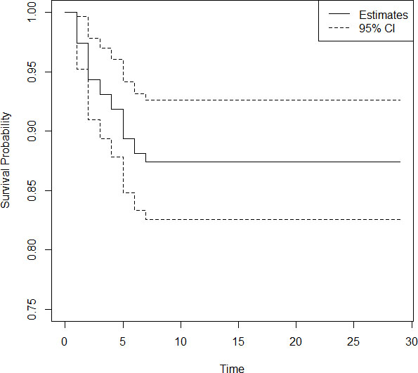
Figure 1.

KM plot of COVID-19 patients in India.

3.Data and results

In this section, we analyse the data on COVID-19 patients in India, using statistical methods explained in Section 2. Since the response variable is time (number of days in hospital) in this study, to employ lifetime data models we need information on the ‘date of confirmation of the disease’ and ‘date of status change’. The available information in the file ‘patient raw data’ from the site ‘https://api.covid19india.org’ as of 19 May 2020 is used to carry out the analysis. From the raw data, we can see that 10.83% of lifetimes are the actually observed lifetimes (current status of the patient is death due to COVID-19) and the remaining 89.17% of lifetimes are censored (current status of the patient is recovered/hospitalized). Since in this study, our interest is focused on death due to COVID-19, the lifetimes of patients deceased due to any reason other than COVID-19 is also considered as a censored lifetime.

We plot a Kaplan Meier curve using the Eq. (5) given in Section 2, to get a basic information about the presence of long term survivors in the data. The minimum value of survival probability estimated is 0.874 with a standard error 0.0114. The plot of KM curve is given in Fig. 1. From Fig. 1 it is evident that, a large fraction of patients will be long term survivors in the data. We analyse the above data to estimate the cure fraction in presence of covariates gender and age. A separate analysis is done for both covariates, since for some patients information on gender, and for some others information on age is missing. First, we estimate the cure fraction considering the covariate gender. In the accessible data, 24.6% are females and the remaining 73.4% are males. We denote females by 0 and males by 1 in the analysis. The estimate of regression parameter is obtained as 0.386. Since the parameter value is greater than 0 it implies that females have greater survival probability than males. The cure fraction of the data is estimated as 0.8840. Survival probability predicted using this model is plotted separately for males and females. The plot of the same is given in Fig. 2.

Figure 2.

Predicted survival probability of males and females.

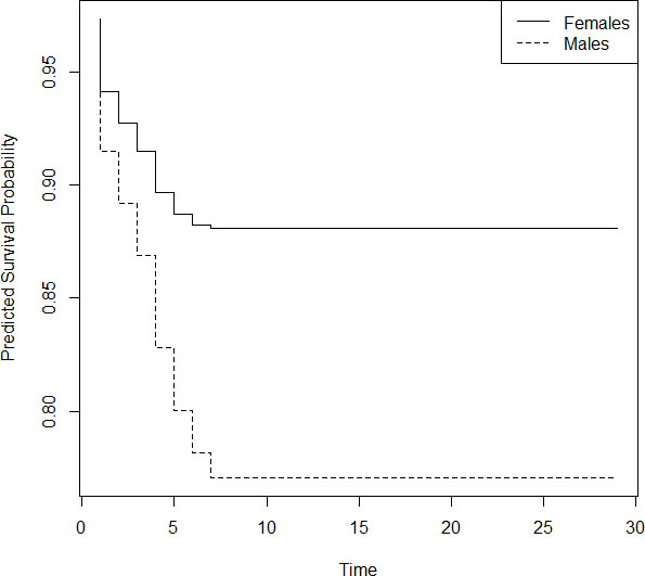
From Fig. 2, we can see that females have a greater survival probability than males; a fact reported by other researchers also. We further note that the survival probability for females becomes constant by day 8 and the value is 0.88. In the case of males, the constancy in survival probability is achieved by day 7 and the value is 0.76.

We now consider the covariate age to estimate the cure fraction. The minimum recorded age is 1 and the maximum is 96. The regression parameter is estimated as 0.2381, which means that the hazard ratio will be greater than 1. Hence age can be treated as a ‘bad prognostic factor’ which tells us that as age increases hazard will increase. The cure fraction is estimated to be 0.9313 with respect to age. We plot the survival probability curve for patients by dividing them into two groups with respect to age; below 60 years and equal to or above 60 years. The value 60 is chosen to determine, how much the survival pattern is different for senior citizens and others. The estimated survival probability is plotted in Fig. 3.

Figure 3.

Predicted survival probability of patients above and below 60 years.

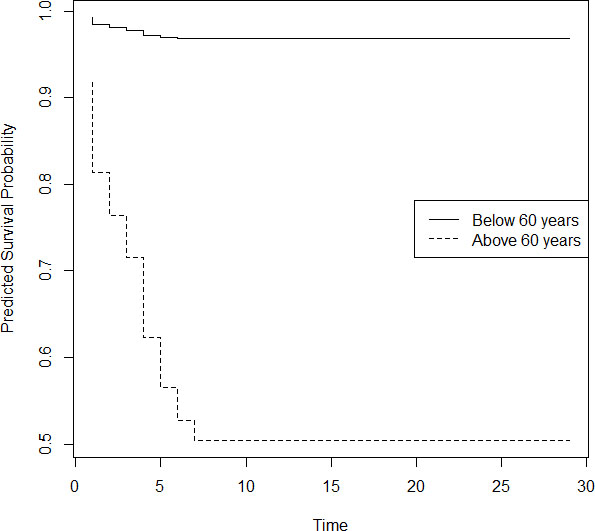
We can see from Fig. 3 that, there is a significant difference in the pattern of survival probabilities for senior people and others. For aged people, survival probability became constant after 7 days and it is only 0.5, while for others survival probability attains stability by day 7 and the value is 0.98. This shows that almost all patients of age below 60 are recovering from COVID-19, while nearly half of the aged people are surviving the disease.

4.Concluding remarks

We analysed the data on COVID-19 patients in India using statistical methods in lifetime data analysis. All the reported statistical studies on COVID-19 data from various nations use compartmental models in epidemiology. We developed a cure rate model to analyse data on COVID-19 patients in India and estimated the proportion of long term survivors in the data in presence of comorbidities age and gender. It is shown that female patients have a greater chance of survival than male patients. Further, the survival probability of the younger population is more than 0.95, while for the aged population it is around 0.5 only.

A COVID-19 patient may be diagnosed with the disease at a later date after infection. In such cases, the exact date of infection may not be known. This possibility of partial information on lifetime leads to the data with left censoring. Our study can be extended to incorporate left censored lifetimes. The models using for the analysis of grouped data, where the lifetimes are grouped into several non-overlapping groups can be used to analyse COVID-19 patient data. Studies in these directions will be reported elsewhere. In addition, it will be worthwhile to analyse the data on COVID-19 patients in presence of information on the current health condition of the patient, since patients with cardiac problems and diabetes may have a greater hazard rate. If the cause of death of a COVID-19 patient can be attributed to any reason other than COVID-19, competing risk models can be developed to explore COVID-19 patient data. A study in this direction will be done separately.

References

[1] | Boag, J. W. ((1949) ). Maximum likelihood estimates of the proportion of patients cured by cancer therapy. Journal of Royal Statistical Society-Series B, 11: (1), 15-53. |
[2] | Cai, C., Zou, Y., Peng, Y., & Zhang, J. ((2012) ). An R-Package for estimating semiparametric mixture cure models. Computer Methods and Programs in Biomedicine, 108: (3), 1255-1260. |
[3] | Cole, S. R., & Hudgens, H. G. ((2010) ). Survival analysis in infectious disease research: Describing events in time. AIDS, 24: (16), 2423-2431. |
[4] | Cox, D. R. ((1972) ). Regression models and life tables. Journal of the Royal Statistical Society – Series B, 34: (2), 187-220. |
[5] | Farewell, V. T. ((1982) ). The use of mixture models for the analysis of survival data with long-term survivors. Biometrics, 38: (4), 1041-1046. |
[6] | Kaplan, E. L., & Meier, P. ((1958) ). Nonparametric estimation from incomplete observations. Journal of the American Statistical Association, 53: (282), 457-481. |
[7] | Lee, E. T., & Go, O. T. ((1997) ). Survival analysis in public health research. Annual Review of Public Health, 18: (1), 105-134. |
[8] | Maller, R., & Zhao, X. ((1996) ). Survival Analysis with Long-Term Survivors, Wiley, New York. |
[9] | Nadia, A. R., & Hazem, A. N. ((2020) ). Data analysis of coronavirus COVID-19 epidemic in South Korea based on recovered and death cases. Journal of Medical Virology, DOI: 10.1002/jmv.25850. |
[10] | Othus, M., Barlogie, B., LeBlanc, M. L., & Crowley, J. J. ((2012) ). Cure models as a useful statistical tool for analysing survival. Clinical Cancer Research, 18: (14), 3731-3736. |
[11] | Peng, Y., & Dear, K. B. G. ((2000) ). A nonparametric mixture model for cure rate estimation. Biometrics, 56: (1), 237-243. |
[12] | Stoltenberg, E. A., Nordeng, H. M., Ystrom, E., & Samuelsen, S. O. ((2020) ). The cure model in perinatal epidemiology. Statistical Methods in Medical Research, DOI: 10.1177/0962280220904092. |
[13] | Sy, P. & Taylor, M. G. ((2000) ). Estimation in a Cox proportional hazards cure model. Biometrics, 56: (1), 227-236. |
[14] | Waqas, M., Farooq, M., Ahmad, R., & Ahmad, A. ((2020) ). Analysis and prediction of COVID-19 pandemic in Pakistan using time-dependent SIR model. arXiv preprint arXiv:2005.02353. The data available on the following websites are used in this study. https://www.worldometers.info/coronavirus/worldwide-graphs https://www.covid19india.org https://api.covid19india.org |