Modeling COVID-19 positivity rates and hospitalizations in Texas

2.1Data

We used records on the 7-day COVID-19 positivity rate by specimen date and the number of persons hospitalized with COVID-19 provided by the Texas Department of State Health Services (2020a). This dataset comes with some caveats and limitations, in particular the disclaimer that “all data are provisional and subject to change.” Examples of limitations include:

2.2Models

Joinpoint Regression is a piecewise regression model that is widely used to capture trends in the data. The model identifies the significant points in the data where the trend changes. The model is popular in estimating the mortality and incidence of cancer trends. The two stage Bayesian joinpoint model applied in this study is an advancement of the previous models used to estimate cancer rates (Ghosh et al., 2009; Kafle et al., 2014). Let yi,i=1,2,…,m be the number of COVID confirmed cases from ni tests performed on a day ti,i=1,2,…,m. Let there be K change points that describe the behavior of the confirmed COVID-19 cases (yi) as a function of time (ti,i=1,2,…,m) and we assumed 0⩽K⩽5. Then the counts yi at time ti,i=1,2,…,m can be modeled by using the Poisson probability distribution as follows:

where t¯ is the mean of ti, τk is the location of kth change point, γk gives the change of slope at the kth joinpoint and (ti-τk)+=ti-τk if ti-τk>0 and zero otherwise.

The previous equation was modified to find the estimated rate of confirmed cases on a given day:

The assumption of joinpoints in our model is random so all parameters in the above models were fitted using the Bayesian methods. For k=K(=5) fixed, we applied a Bayesian Model Selection (BMA) criteria to select the best model among K+1 nested models. These K+1 nested models have some common parameters. We can only assign the same priors to all common parameters in all the nested models if they have the same meaning (Berger & Pericchi, 2001). To overcome this issue we adopted the alternative reparametrization method proposed by Martinez-Beneito et al. (2011). The reparametrized model is as given below:

where δ is the binary indicators for the k breakpoints in the model as follows:

The parameters in the above models were fitted using the Bayesian methods as explained in Kafle et al. (2014). We estimated Daily Percentage Change (DPC) to detect the rate of change of confirmed cases in the model using the following formula:

We fitted the second stage model to study the rate of hospitalization in the population using the fitted COVID-19 rates from the first stage as one of the covariates and estimated the lag time in hospitalization. Let hi,i=1,2,…,m be the observed hospitalization counts of COVID patients in the population at time (ti,i=1,2,…,m). Again, using the same assumptions as above, the hospitalization hi at time ti,i=1,2,…,m can be modeled as

Here Ni is the total population at time (ti,i=1,2,…,m), rateie is the estimated confirmed cases from the first stage model, ψ is time lag, and ci’s are the coefficients.

The above model is used to estimate the rate of hospitalization (h⁢ri) and lag time, as a function of positivity below:

Here h⁢ri is the hospitalization rate, rateie is the estimated confirmed cases from the first stage model, ψ is time lag, and ci’s are the coefficients. The estimation of the lag time in hospitalization in our model is motivated by the extension of the model (Ghosh et al., 2009) and assumed a prior to be uniformly distributed between 3 and 15 days, consistent with previous estimates of the disease progression (Linton et al., 2020; Yang et al., 2020). The parameter estimates and detection of change points in this model were obtained using the same approach as explained above using the following model:

3.1Test positivity rates

As shown in Fig. 1, the analysis identified four joinpoints that can be tied anecdotally to statewide initiatives and behavior changes: May 31, June 19, July 4 and September 21. Texas Department of State Health Services (2020b), reports a list of executive orders issued in response to the pandemic during this time period. According to the Centers for Disease Control (2020), the mean time from infection to symptom onset is 6 days, and the median number of days from symptom onset to COVID-19 test among positive patients is 3 days. Thus, changes in test positivity rates can be expected roughly 9 days after behavioral shifts.

Figure 1.

Daily rates of COVID-19 confirmed cases.

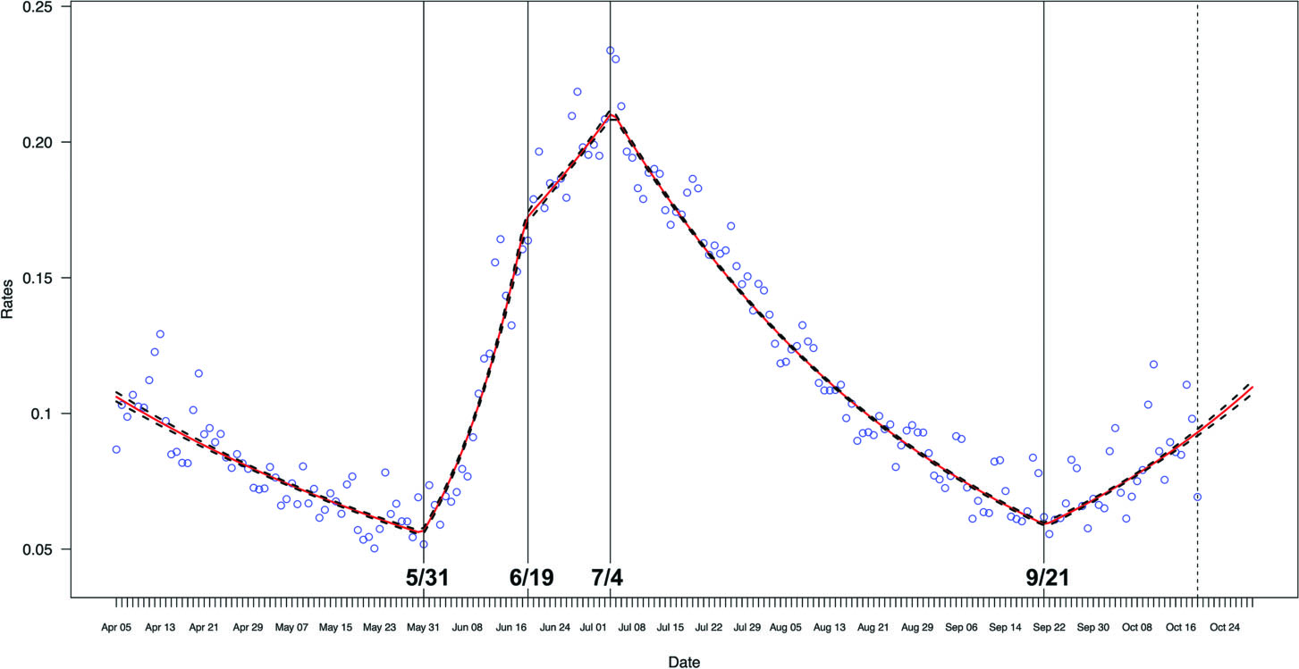
On April 2, a statewide stay at home order began. Bars, malls, retailers, and gyms shut down. Restaurants were allowed to stay open, but only for to-go orders. This order was highly effective in reducing the positivity rate of COVID-19 tests beginning April 5. On May 1, Texas began reopening. Texas reopened restaurants (to 25% capacity) on May 1, reopened offices and gyms (to 25% capacity) on May 18, and reopened bars (to 25% capacity) on May 22. Texas also expanded restaurants to 50% capacity on May 22. Nine days later, May 31, was identified as the first joinpoint in the model as the COVID-19 positivity rate in Texas began increasing steeply. Texas continued reopening in June as the positivity rate increased, although the slope shifted at a second joinpoint of June 19. On June 22, Governor Abbott implored Texans to distance and wear masks (Svitek, 2020). On June 26, bars in Texas were ordered to close except for delivery and take-out, and restaurants were reduced from 75% to 50% capacity. Eight days later, July 4, the COVID-19 positivity rate began to decline. Additionally, on July 2 the governor issued an order requiring masking in public spaces, “with few exceptions,” solidifying the downward trend. Universities across Texas reopened the weeks of August 17 and August 24 (ABC13 Eyewitness News, 2020, August 19), while K – 12 school districts opened for in person schooling on dates ranging from September 8 to October 13 (Swaby & Platoff, 2020, September 8). Not surprisingly, the model detected a reversal of the downward trend in incidence on September 21. Thus behavioral shifts do appear to pre-date breakpoints, although these observations are strictly anecdotal.

The mean, standard deviation, Monte Carlo errors, and associated 95% credible intervals for Test Positivity Rates model were presented in the table below.

3.2Hospitalization rates

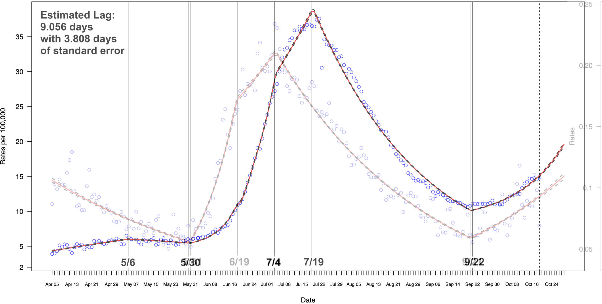
In addition to the insights the first stage model provided for the impact of behavior changes, it informed the second stage model, using the estimated positivity rate to estimate the hospitalization rate, as well as the time to hospitalization, in the Texas population. The estimated positivity rate from the first stage model accurately modeled the hospitalization rates in the second stage (Fig. 2), with joinpoints at May 6, May 30, July 4, July 19 and September 22. As expected, both graphs have the same overall shape, with the exception of the first segments of each graph: The daily positivity rate of COVID-19 cases falls from April 5 to May 31, whereas the daily hospitalization numbers are roughly rising or flat over this time period. We believe that the primary reason for this deviation is the relatively small number of tests conducted during this time period: From April 5-30, Texas conducted an average of 11081 tests per day, whereas during May, Texas conducted an average of 24674 tests per day. In the months of June and July, the average number of tests per day were 44723 and 61671, respectively. Average daily tests have been above 35000 in each month since. We believe that the small number of daily tests during April and May resulted in an artificially high positivity rate (relative to the rest of the time series) at the beginning of the time series. The estimated lag time between a change in positivity rates across Texas and hospitalization rates is 9.056 days, with a standard error of 3.808. The lag estimate and associated standard error appear to support the conclusions of Yang et al. (2020) who found a median of 9.5 (± 2.5) days between symptom onset and ICU among patients in Wuhan early in the outbreak. The additional error in the model of Texas patients incorporates the additional variability currently associated with access to testing for asymptomatic, symptomatic and significantly ill COVID-19 positive Texans.

Figure 2.

Daily Hospitalization Rates Due to COVID-19 and Test Positivity Rates Combined.

The mean, standard deviation, Monte Carlo errors, and associated 95% credible intervals for Hospitalization Rates model were presented in the table below.

References

[1] | ABC13 Eyewitness News ((2020) ). Texas colleges and universities’ fall 2020 plans. Available at https://abc13.com/college-back-to-school-plan-university-online-fall-2020/6350823. |
[2] | Berger, J. O., & Pericchi, L. R. ((2001) ). Objective bayesian methods for model selection: introduction and comparison. Lecture Notes-Monograph Series, 38: 135-207. |
[3] | Centers for Disease Control and Prevention ((2020) ). COVID-19 pandemic planning scenarios. Available at https://www.cdc.gov/coronavirus/2019-ncov/hcp/planning-scenarios.html. |
[4] | Ghosh, P., Basu, S., & Tiwari, R. C. ((2009) ). Bayesian analysis of cancer rates from SEER program using parametric and semiparametric joinpoint regression models. Journal of the American Statistical Association, 104: (486), 439-452. |
[5] | Kafle, R. C., Khanal, N., & Tsokos, C. P. ((2014) ). Bayesian age-stratified joinpoint regression model: An application to lung and brain cancer mortality. Journal of Applied Statistics, 41: (12), 2727-2742. |
[6] | Keskinocak, P., Orac, B. E., Baxter, A., Asplund, J., & Serbun, N. ((2020) ). Impact of social distancing on COVID 19 spread: State of Georgia case study. PLoS One, 15(10). |
[7] | Linton, N. M., Kobayashi, T., Yang, Y., Hayashi, K., Akhmetzhanov, A. R., Jung, S. M., Yuan, B., Kinoshita, R., & Nishiura, H. ((2020) ). Incubation period and other epidemiological characteristics of 2019 novel coronavirus infections with right truncation: A statistical analysis of publicly available case data. Journal of Clinical Medicine, 9: (2), 538. |
[8] | Martinez-Beneito, M. A., García-Donato, G., & Salmerón, D. ((2011) ). A Bayesian joinpoint regression model with an unknown number of break-points. Annals of Applied Statistics, 5: (3), 2150-2168. |
[9] | Svitek, P. ((2020) ). Gov. Greg Abbott urges voluntary measures to curb coronavirus spread but says closing Texas will be “the last option”. The Texas Tribune. Available at https://www.texastribune.org/2020/06/22/texas-coronavirus-greg-abbott-press-conference/. |
[10] | Swaby, A., & Platoff, E. ((2020) ). Many Texas students will return to classrooms Tuesday. Little will be normal. The Texas Tribune. Available at https://www.texastribune.org/2020/09/08/texas-schools-reopening-in-person/. |
[11] | Texas Department of State Health Services ((2020) a). Accessible version (Excel). Available at https://dshs.texas.gov/news/updates.shtm. |
[12] | Texas Department of State Health Services ((2020) b). Opening the state of Texas. Available at https://www.dshs.state.tx.us/coronavirus/opentexas.aspx. |
[13] | Yang, X., Yu, Y., Xu, J., Shu, H., Xia, J., Liu, H., Wu, Y., Zhang, L., Yu, Z., Fang, M., Yu, T., Wang, Y., Pan, S., Zou, X., Yuan, S., & Shang, Y. ((2020) ). Clinical course and outcomes of critically ill patients with SARS-CoV-2 pneumonia in Wuhan, China: a single-centered, retrospective, observational study. The Lancet Respiratory Medicine, 8: (5), 475-481. |