
A versatile laboratory setup for high resolution X-ray phase contrast tomography and scintillator characterization
Abstract
BACKGROUND:
X-ray micro-tomography (μCT) is a powerful non-destructive 3D imaging method applied in many scientific fields. In combination with propagation-based phase-contrast, the method is suitable for samples with low absorption contrast. Phase contrast tomography has become available in the lab with the ongoing development of micro-focused tube sources, but it requires sensitive and high-resolution X-ray detectors. The development of novel scintillation detectors, particularly for microscopy, requires more flexibility than available in commercial tomography systems.
OBJECTIVE:
We aim to develop a compact, flexible, and versatile μCT laboratory setup that combines absorption and phase contrast imaging as well as the option to use it for scintillator characterization. Here, we present details on the design and implementation of the setup.
METHODS:
We used the setup for μCT in absorption and propagation-based phase-contrast mode, as well as to study a perovskite scintillator.
RESULTS:
We show the 2D and 3D performance in absorption and phase contrast mode, as well as how the setup can be used for testing new scintillator materials in a realistic imaging environment. A spatial resolution of around 1.3μm is measured in 2D and 3D.
CONCLUSIONS:
The setup meets the needs for common absorption μCT applications and offers increased contrast in phase contrast mode. The availability of a versatile laboratory μCT setup allows not only for easy access to tomographic measurements, but also enables a prompt monitoring and feedback beneficial for advances in scintillator fabrication.
1Introduction
X-ray micro-tomography (μCT) has become a well-established method for non-destructive 3D imaging [52]. The high penetration depths of X-rays in many materials allows for the reconstruction of volume information from a series of 2D projection images, revealing the inner structure of the sample. This makes it an attractive technique whenever the integrity of the sample is crucial, as e.g. in bio-medical imaging [11, 23, 28, 35, 45], archaeometry [38, 40], paleontology [13], industrial quality control [7, 33], and material science [14, 42].
Besides relying on the contrast given by the local absorption coefficients in the sample, it is possible to use the phase shift as an additional contrast mechanism [12, 50]. This is especially useful for low-Z materials, which often have weak absorption and thus weak contrast, but still cause significant phase shifts [18]. Multiple techniques to access phase information have been proposed, among others interferometric [5, 27, 34, 36, 39], crystal-analyzer-based [6], speckle [53, 54], and Zernike techniques [19]. In contrast to these techniques, propagation-based phase-contrast imaging (PB-PCI) does not need any additional optical elements to encode/decode the phase information. Given enough coherence of the incoming wave, a small in-line propagation distance between sample and detector allows for interference between phase shifted parts of the wave, resulting in detectable intensity modulations. Even though the technique is common at synchrotron sources, the requirements on coherence, monochromaticity and brilliance of the source are moderate, making this method also feasible [51]. It is especially beneficial for setups using micro-focus X-ray tubes where the flux is low, but some spatial coherence is provided. As with other phase contrast methods, PB-PCI can be used for bio-medical samples [10, 15, 46]
Even though synchrotron setups still outperform lab systems in terms of resolution and speed, a lab setup comes with the considerable benefit of easy accessibility and experimental flexibility. High resolution scintillator detectors and micro-focus sources provide resolutions in the micrometer range, which is often sufficient for applications from biology or material science, whereas new nano-focus lab sources are pushing for sub-micron resolution [10, 29].
In μCT systems, the scintillators are often the bottleneck for spatial resolution, signal-to-noise ratio, and measurement speed. Since a high resolution requires thin scintillators, the materials need a high X-ray absorption coefficient (stopping power) in the right energy range, as well as a good conversion efficiency to provide sufficient sensitivity [22, 25]. Moreover, temporal effects such as afterglow and degradation can pose a problem for serial imaging, i.e., in tomography [26]. The development and testing of cost-efficient scintillators with a high stopping power (high-Z), high light yield, low afterglow, high stability, and low detection limit is thus of great research interest for X-ray microscopy. Scintillator development is a growing field, fueled by the increasing demand for of X-ray imaging detectors as well as constantly evolving fabrication and synthesis methods [26]. Many different materials are currently studied, such as powders, single crystals, structured arrays, nano crystals and ceramics [26]. Recently, metal halide perovskites (MHP) have been recognized as a promising candidate for a new generation of scintillators [20, 24].
Even though commercial integrated μCT solutions are available and some are offering a phase contrast mode, they are tailored for labs that focus on a high throughput of samples and often lack the flexibility that a customized setup offers for method development, adjustments for specific imaging tasks and testing of new optical elements and hardware. Integrated commercial systems are also not ideal for educating students on the inner workings of X-ray imaging. To have more flexibility is especially important in the field of scintillator development, since characterizing their performance in realistic lab settings is crucial. Here, we present a custom build X-ray μCT setup that combines traditional absorption μCT, propagation-based phase-contrast tomography (PB-PCT) and the option to be used for scintillator characterization. Alongside the technical specifications and performance measures we show by means of an example application the bottlenecks and recommend design considerations based on the intended use.
2Setup Design
The setup has three main components: a micro-focus X-ray source, a tomography stage, and an X-ray scintillator detector (see Fig. 1a). All three components are flexibly mounted on a passive air-cushioned optical table to reduce vibrations, and can be moved independently from each other. The main design idea was to build a flexible yet compact setup that allows for a wide range of geometries. Since conventional X-ray lab sources are divergent sources, the coherence length and geometrical magnification are influenced by the distance to the source [21]. Depending on source and detector parameters two different geometries are common: source-size-limited (high magnification) or detector-limited (low magnification). For this setup we chose a detector-limited approach where the resolution is limited by the detector point-spread function [16]. The sample is placed relatively close to the detector and the magnification is close to 1. In this geometry a high-resolution detector allows us to use a standard micro-focus source with a source size larger than the detector resolution (up to a few tens of micrometer). Moreover, due to the low magnification, we can assume a parallel beam illumination in the tomography reconstruction. In comparison, high magnification geometries require a source size smaller than the detector resolution and cone beam tomographyreconstructions.
Fig. 1
a) Photo of the tomography setup. From right to left: 1 - source, 2 - sample stage, 3 - high-resolution scintillator detector, 4 - top view USB microscope for monitoring. b) and c) photo of the scintillator mount attached to the objective lens without build-in scintillator: 1 - micrometer screws of kinematic mount, 2 – magnetically attachable scintillator carrier plate with pinhole. Note that the picture in a) shows the detector with a commercial scintillator.

The source is a micro-focus X-ray tube with a water-cooled copper target (Rigaku) and a nominal source spot diameter of 28.1μm (FWHM at 45 V/1 mA). The photon flux of (4.192 ± 0.001) 1010 ph/s on the optical axis at 4.2 cm distance was measured over 64 h with an X-ray diode (xPin, Rigaku) and shows only small fluctuations. A stable illumination position and flux is crucial for μCT measurements that take many images and thus have overall measurement times that can add up to several hours. As specified by the manufacturer the electron spot on the target has a positional and size uncertainty of±1μm, respectively. The exposure time for each image depends on the chosen distances as well as on the sample properties and is in the range of several tens of seconds due to the limited flux. Since the measurement itself runs automatically, these long measurement times only pose a concern if the sample is radiation sensitive or changes over time.
The tomography stage includes five linear axes (SmarAct) and one precision air-bearing rotation stage (LAB RT075S). Two long range linear axes (103 mm, 63 mm travel range) are positioned underneath the rotation stage to align the rotational axis with the vertical center line of the detector and adjust the magnification. The two additional horizontal axes (30 mm travel range) on top of the rotation stage are used to position the sample on the rotation axis. The vertical alignment (21 mm travel range) is done by a linear motor with an angular bracket. It has a maximum lift of about 1.5 N. This 5-axis design allows for greater freedom in sample mounting and the option of stitching sub-volumes of larger samples in zoom-tomography. The sample mount is compatible with standard scanning electron microscopy (SEM) studs. The smallest source-sample distance which still allows for a full tomographic acquisition is 6 cm. The shortest sample-detector distance for tomography is 6 mm. A digital microscope is positioned on top of the sample stage to be able to monitor the alignment remotely (see Fig. 1a).
The rotation is provided by a compact air bearing stage (LAB RT075S) with an encoder resolution of 133μrad. It is crucial for achieving a successful tomographic reconstruction with high resolution to have a radial run-out error smaller than the 2D resolution. For our system, the radial run-out of the combined sample stage was measured interferometrically by the manufacturer and certified to be below 1μm, which fulfils this requirement.
The detector is a high-resolution scintillator-based X-ray camera (XSight, Rigaku) with a CCD of 3296 px (H)×2472 px (V). The objective lens unit of the detector can be easily exchanged to adjust the effective pixel size and field of view (FOV) to the given imaging task. Two commercial lens units are currently in use: L0540 and L2160, providing a pixel size and nominal FOV of 0.55μm/1.76×1.36 mm and 2.14μm/7.05×5.28 mm, respectively. The scintillators build into each lens unit are optimized for the respective resolution and therefore yield slightly different efficiencies. Since information on the exact composition and thickness of the scintillators is not publicly available, the spectral sensitivity is unknown. The manufacturer specifies the energy range from 5–30 keV for both objectives.
2.1Scintillator mount
Besides studying tomography samples, the setup can be used for testing, characterization, and comparison of new scintillator materials. This is done with a modified lens unit with the same optics and the same effective pixel size as lens unit L0540, 0.54μm, but without integrated scintillator, acquired from Rigaku. The focal plane was designed to be 1.2 mm in front of the lens unit, where the scintillator under test should be positioned (see Fig. 1b). Since the depth of focus of the lens unit is less than 5μm, it is necessary to align the scintillator precisely in the focal plane to achieve the best resolution. The scintillator mount can be directly attached to the housing, leaving the rest of the setup unaffected. This compact design allows the sample to be positioned close enough to the scintillator for absorption contrast imaging. The mount is based on an adapted kinematic optics mount and thus provides three micrometer screws for tilting and translating the scintillator plane (see Fig. 1c). It must be noted that only planar scintillators can be properly aligned, due to the small depth of focus. A magnetically attachable metal carrier with a pinhole holds the scintillator itself and can easily be exchanged without disassembling the mount (see Fig. 1c). Moreover, the magnetic attachment of the carrier allows for manual in-plane translation to find a good scintillator area. The alignment of the focal plane can be done by grazing illumination with an UV torch (without X-rays) since the cooled CCD is very sensitive to visible light and most scintillators also react to UV. The option to align without X-rays is helpful when the monitoring of degradation due to X-ray exposure is of interest. When aligned, a 1.2 mm gap remains between detector and scintillator, which makes it crucial to block all ambient light and to perform a proper flat field correction to account for possible straylight.
To better understand the performance of the scintillator, it is important to measure the X-ray excited scintillation spectrum. For this purpose a cooled spectrometer (Ocean Insight QE Pro) is available.
2.2Alignment Procedure without a goniometer
Since no goniometer is used in the setup, the rotation axis is likely to have a tilt along the optical axis (pitch angle) as well as in the detector plane (roll angle) [44]. The roll angle can be easily identified and corrected in the data processing by numerically rotating the images. The pitch angle cannot easily be corrected for in the data processing. It results in each pixel row being the projection along a slightly different slice through the volume for each image, which will cause artifacts in the tomography reconstruction. However, for a small pitch angle and a divergent source, it is possible to compensate for this misalignment by adjusting the optical axis [44]. The source is moved vertically relative to the detector until the new optical axis is perpendicular to the rotation axis and aligned with the center of the detector. Obviously, this entails that the detector is afterwards not perpendicular to the new optical axis anymore and the image will have a slight skew in vertical direction. But usually, the pitch angle of the rotation axis is in the range of 0°–3° and the skew effect thus negligible compared to the resolution limit of the setup (any pitch < 24° results in a skew < 10% of the pixel size).
2.3Software
The data acquisition and motor control were implemented as a Python library, which accesses the APIs of the various hardware components via C bindings or ASCII commands, thus centralizing the handling of the setup. The alignment is performed interactively while monitoring the motor positions via a camera live feed from the alignment microscope (see Fig. 1a) as well as detector images. Afterwards, the tomography acquisition is fully automated and can run unsupervised.
The data processing is also implemented in Python. After the flat field correction, the image stack is saved in a HDF5 format for better memory handling, since the high-resolution datasets easily account to file sizes of several tens of gigabytes. The tomography reconstruction is based on the functions provided by the tomopy package [17] and is performed on a high RAM workstation. Due to the small geometric magnification in our setup, it is enough to use parallel beam algorithms. A variety of pre-processing steps such as tilt correction, stripe removal [48] and phase retrieval [3] are implemented as options in the workflow and can be applied to the data as deemed necessary.
3Methods
3.1Spatial resolution
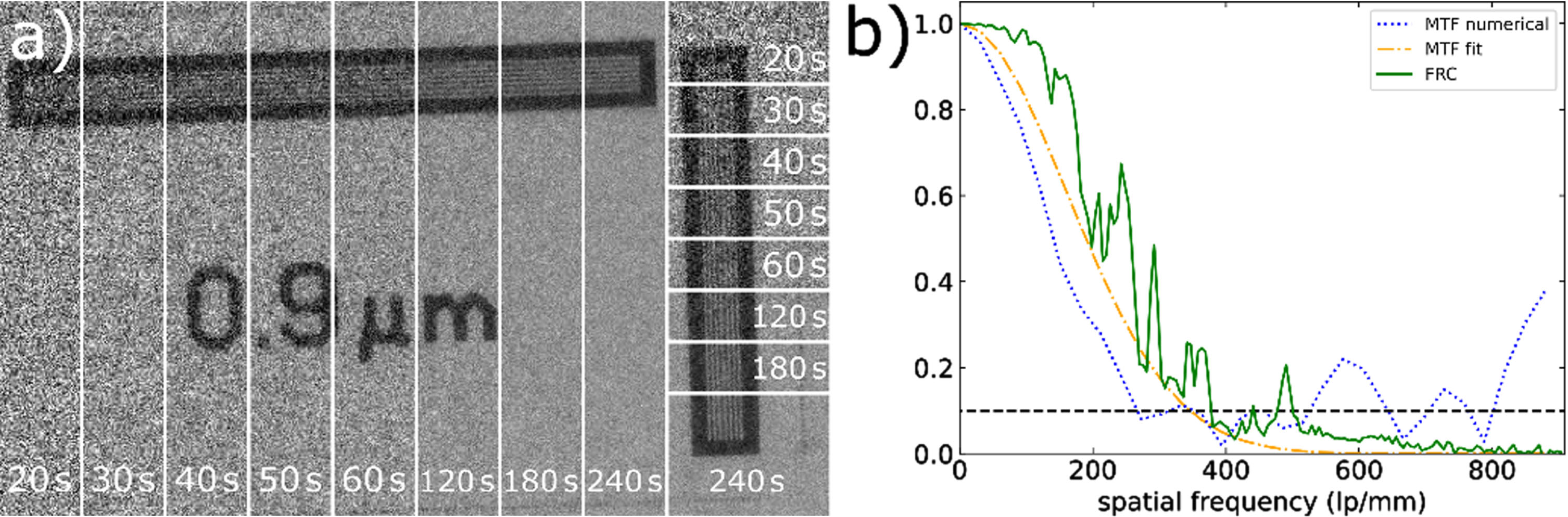
To provide a comparable value for the spatial resolution we choose to use the standard resolution chart Rt RC-02b from the Japanese Institute of Metrology (JIMA) and extract the resolution with three different approaches: the smallest visible bar pattern, the modulation transfer function (MTF) based on the slanted edge method and the Fourier Ring correlation (FRC) between two independent measurements of the JIMA. Since the resolution also depends on the signal-to-noise ratio (SNR), we extracted the resolution dependent on the exposure time varying from 20–240 s, shownin the SI.
The MTF is defined as the Fourier transform of the line spread function (LSF), which is the one-dimensional gradient over the edge spread function (ESF). To provide enough oversampling of the edge the slanted-edge method was used [4]. The MTF calculation can be done either numerically or by fitting a function, e.g., a Gaussian error function, into the data and then analytically deriving the resolution from the fit parameters [29, 41]. The fit-based approach avoids artifacts from the numerical derivative and Fourier transform, but by choosing the fit function it also restricts the model and ignores all textures in the noise. We compare both approaches on the same data.
The numerical MTF was calculated for the average of 5 consecutive oversampled lineouts extracted from a vertical edge in the 15μm bar pattern of the JIMA (Fig. 2b), as described in [4]. The averaging is necessary to suppress the high frequency noise before it gets amplified by the numerical gradient used to calculate the LSF [4]. Moreover, we used a Kaiser window (β = 14) for apodization.
Fig. 2
a) 0.9μm bar pattern of the JIMA for different exposure times from 20 s–240 s. With increasing exposure time, the bars become clearly distinguishable. More than 60 s exposure gives only small improvements. b) MTF and FRC extracted from a 240 s image of the JIMA. Both fitted MTF and FRC yield a similar resolution of 350–380 lp/mm at the 10% threshold, while the numerical MTF only results in around 270 lp/mm due to the noise.
For the fit-based MTF calculation a Gaussian error function was fitted into the same lineouts. The fit parameter σ is proportional to the width of the edge and thus the resolution. A weighted average of all σ extracted from the individually fitted lineouts was used in the following calculations. Using the 10% threshold, the resolving power is described by the frequency
Additionally, the FRC can be used to estimate the resolution. It measures the similarity between two independent measurements of the same image information and is defined as the cross-correlation between the measurements normalized by the square root of the product of the auto-correlations of each image, summed over radial frequency bins [47].
3.2Phase Contrast
Propagation-based phase-contrast imaging (PB-PCI) relies on the near field self-interference of the exit wave upon propagation after the sample [51]. By introducing a small propagation distance between sample and detector, bright and dark fringes can be observed around interfaces in the sample. This is commonly referred to as “edge-enhancement.” A suitable range of propagation distances z2, for edge enhancement is given by the Fresnel number
To retrieve an image proportional to the projected electron density of the sample, several phase retrieval approaches for PB-PCI are available. One of the most convenient and widespread tools is the so-called Paganin filter [32]. It is based on an inversion of the TIE and was originally derived for samples consisting of a single material and monochromatic illumination. It has been shown that it can be generalized for polychromatic setups [1, 37] by defining an effective refractive index, based on the weighted spectrum of the source. This makes it applicable in X-ray tube setups. From a flat field corrected transmission image Iproj = I (x, y, z = z2)/I0 measured at distance zeff, the integrated thickness of the object is retrieved by a series of filtered Fourier transforms
3.3Tomography
For the tomogram we used a magnification of 1.1 for high phase contrast [8]. 1200 projections with an angular step of 0.15° and 60 s exposure per image were taken over 180°. Each projection was flat field corrected, and then phase retrieved using the Paganin filter with δ/β = 5e-5. The volume was reconstructed with the filtered back projection (FBP) algorithm implemented in tomopy [17], using the Hamming filter.
The Fourier shell correlation (FSC) was calculated on a 300×300 px subset of the volume and apodization with the Kaiser filter (β = 10) was performed to avoid artefacts from the volume boundaries.
4Results and discussion
4.1Spatial resolution
The spatial resolution is one of the main metrics to characterize the performance of any imaging system. It depends on the source spot size and stability, detector point spread function and noise, as well as the overall stability of the setup.
Figure 2a shows the 0.9μm bar pattern of the JIMA for different exposure times. As the SNR increases with exposure time the visibility of the lines and spaces improves and above 60 s the 0.9 μm bars are clearly distinguishable, both vertically and horizontally.
Figure 2b shows the resolution curves for the three different approaches (240 s exposure time): numerical MTF, fit-based MTF and FRC. The numerical MTF crosses the 10% criterium at 270 lp/mm, corresponding to 1.9 μm per single line. The fit-based MTF estimates the resolution to (360 ± 20) lp/mm, corresponding to (1.39 ± 0.03) μm. The FRC with the same data and resolution threshold, yields 380 lp/mm, corresponding to 1.3μm, which agrees well with the results from the fit-based MTF. The numerical MTF is still showing artefacts from the noise, especially for low exposure times and only gives an unreliable estimate of the resolution (other exposure times see SI). Like the observation of the bar visibility in the JIMA itself (Fig. 2a), the resolution improves with exposure time but stays more constant for exposures > 60 s (see SI). The discrepancy between the three resolution estimates illustrates that the evaluation of resolution is non-trivial and depends strongly on the chosen method and image noise. For noisy images, the fitted MTF and FRC are more consistent. In real imaging, the resolution will furthermore depend on the density and gradients in the sample.
4.2Absorption and PB-PC tomography
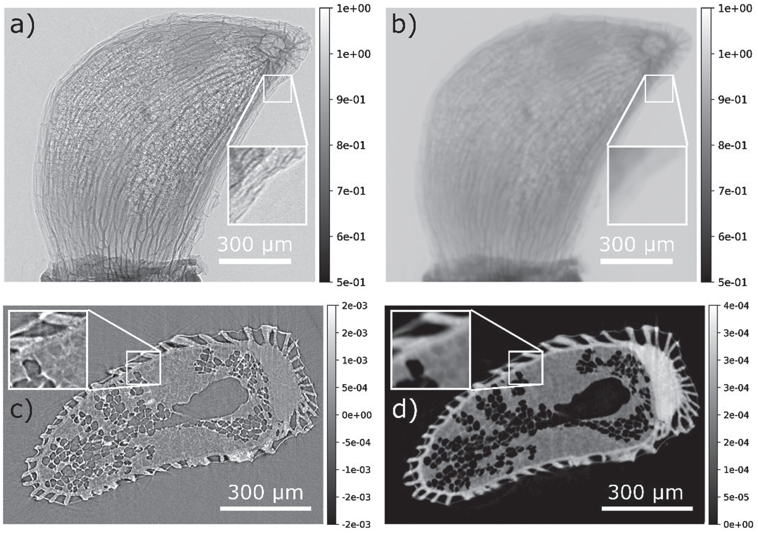
Examples of the projections and slices of a tomogram of a blueberry seed recorded with this setup are shown in Fig. 3. As can be seen in Fig. 3b the phase retrieval acts like a smoothing filter but increases the image contrast, so that areas like the shell of the seed with low absorption contrast (Fig. 3c/d) become more distinct. Since this sample already shows relatively good absorption contrast, phase contrast imaging is not strictly necessary, but it illustrates the capabilities of the setup.
Fig. 3
PB-PCI tomogram of a blueberry seed. a) Flat field corrected projection image. Note the pronounced edge enhancement fringes (see inset). b) Paganin phase retrieved projection. Note the suppression of the fringes and loss of resolution. c) Slice through the reconstructed volume without prior phase retrieval. The fringes are now part of the reconstruction, impeding with segmentation and data interpretation. d) Slice through the reconstruction of priorly phase retrieved projections. Note the increased contrast and noise suppression.
The spatial resolution in 3D was measured by calculating the Fourier shell correlation (FSC), which is the 3D equivalent of the FRC, of two independent reconstructions, each using alternating projections of the original dataset, with phase retrieval. This yields a resolution of around 400 lp/mm, similar to the 2D case. Since in our setup the spatial resolution is around 3x the pixel size, the low-pass filter of the phase retrieval does not reduce the resolution but dampens the high frequency noise and increases the contrast. We also observe a rise of the FSC towards very high frequencies, which implies a correlation of the two reconstructions in the high frequencies. This does not mean the resolution is higher than the value derived from the first crossing of the threshold. The correlation of high frequencies rather indicates reconstruction artefacts. These could be a similar noise spectrum due to the flat field correction, since the same set of dark and bright images was used for both subsets, or ring and streak artefacts.
4.3Tomography with new scintillator
Using the objective lens without built-in scintillator (see Fig. 1b/c), it is possible to perform tomography measurements with different scintillators, to characterize their performance under realistic measurement conditions. Being able to do such tests in-house, quickly, and repeatedly after the fabrication provides valuable information about the performance and degradation, as well as it helps to develop suitable handling and fabrication strategies, that otherwise would require many beamtimes at a synchrotron.
As an example for the feasibility of such tests, we studied a scintillator composed of CsPbBr3 metal halide perovskite nanowires grown in an anodized aluminum oxide (AAO) membrane [9, 55]. One of the main challenges for perovskite materials is the low stability and sensitivity to humidity, temperature, and radiation damage, which up to now keeps them from being used in commercial systems [20, 49]. Therefore, it has been difficult to acquire a full, high-resolution tomogram with a perovskite scintillator without noticeable degradation during the measurement time. This has been achieved now with our setup and scintillator [9].
Fig. 4
Fourier shell correlation (FSC) for a sub-volume within the phase-retrieved blueberry tomogram. The resolution is estimated to be 400 lp/mm.
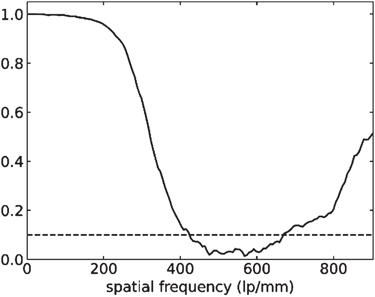
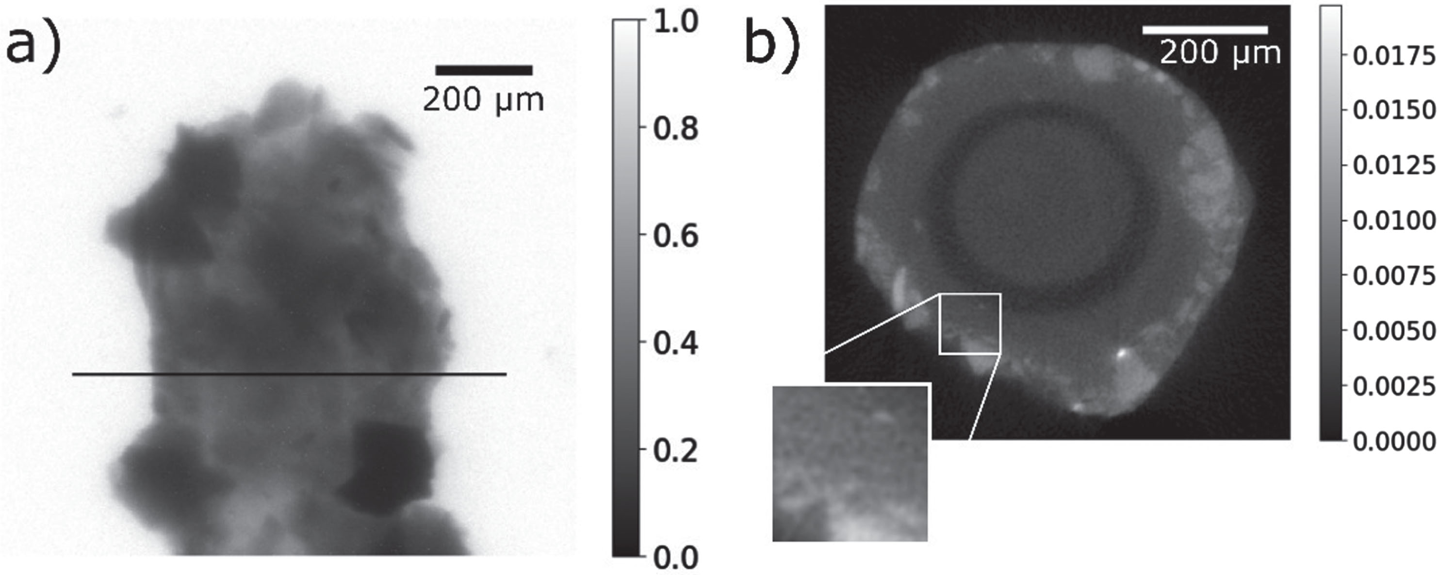
Figure 5a shows a projection image of rock grains from the Siljan meteoroid impact side, mounted in vacuum grease on a Kapton tube. The sample was measured in absorption, since the rock grains show strong attenuation. A slice through the reconstruction in Fig. 5b shows grains down to about 10μm diameter, illustrating the resolution. Moreover we were able to monitor the influence of humidity and integrated dose on the light yield and resolution over long time scales [9].
Fig. 5
Tomography of rock grains mounted on a Kapton tube, recorded with a CsPbBr3 nanowire in AAO scintillator. a) Projection image after flat-field correction. The dataset was binned with a factor of 4 before reconstruction. The black line indicates the slice through the reconstructed volume shown in b). The side length of the inset is 100 μm. A 10 μm grain is visible.
5Conclusion
In conclusion, we have presented a compact, versatile, and flexible X-ray μCT lab system, which provides absorption and phase contrast imaging modalities as well as the option to be used for scintillator characterization. We have shown that the spatial resolution is around 1.3 μm both in 2D and 3D, which is comparable to commercial μCT setups. Furthermore, we demonstrated how the introduction of a propagation distance after the sample can help to improve the contrast. Finally, the setup was used for characterizing a new scintillator material in a realistic experimental setting. The possibility to test state-of-the-art scintillators in a continuous feedback mode with tuning the fabrication parameters is an important contribution to accelerating developments in material science.
Acknowledgments
We thank Zhaojun Zhang for the perovskite scintillator. This project received funding from the European Research Council (ERC) under the European Union’s Horizon 2020 research and innovation program (Grant 801847). Moreover, this research was also funded by the Olle Engkvist Foundation, the Crafoord foundation and NanoLund.
SUPPLEMENTARY MATERIAL
[1] The supplementary material is available in the electronic version of this article: https://dx.doi.org/10.3233/XST-221294.
REFERENCES
[1] | Arhatari B.D. , et al., Phase Imaging Using A Polychromatic X-ray Laboratory Source, Opt Express 16: ((2008) ), 19950–19956. |
[2] | Bartels M. , et al., Phase contrast tomography of the mouse cochlea at microfocus x-ray sources, Applied Physics Letters 103: (8) ((2013) ), 083703. |
[3] | Beltran M.A. , Paganin D.M. and Pelliccia D. , Phase-and-amplitude recovery from a single phase-contrast image using partially spatially coherent x-ray radiation, Journal of Optics 20: (5) ((2018) ), 055605. |
[4] | Buhr E. , Gunther-Kohfahl S. and Neitzel U. , Accuracy of a simple method for deriving the presampled modulation transfer function of a digital radiographic system from an edge image, Med Phys 30: (9) ((2003) ), 2323–2331. |
[5] | David C. , et al., Differential x-ray phase contrast imaging using a shearing interferometer, Applied Physics Letters 81: (17) ((2002) ), 3287–3289. |
[6] | Davis T.J. , et al., Phase-contrast imaging of weakly absorbing materials using hard X-rays, Nature 373: ((1995) ), 595. |
[7] | De Chiffre L. , et al., Industrial applications of computed tomography, CIRP Annals 63: (2) ((2014) ), 655–677. |
[8] | Dierks H. and Wallentin J. , Experimental optimization of X-ray propagation-based phase contrast imaging geometry, Opt Express 28: (20) ((2020) ), 29562–29575. |
[9] | Dierks H. , et al., 3D X-ray microscopy with a CsPbBr3 nanowire scintillator, Nano Research 2022. |
[10] | Eckermann M. , et al., Phase-contrast x-ray tomography of neuronal tissue at laboratory sources with submicron resolution, J Med Imaging (Bellingham) 7: (1) ((2020) ), 013502. |
[11] | Eckermann M. , et al., Three-dimensional virtual histology of the cerebral cortex based on phase-contrast X-ray tomography, Biomedical Optics Express 12: (12) ((2021) ), 7582–7598. |
[12] | Endrizzi M. , X-ray phase-contrast imaging. Nuclear Instruments and Methods in Physics Research Section A: Accelerators, Spectrometers, Detectors and Associated Equipment 878: ((2018) ), 88–98. |
[13] | Erb A. and Turner A.H. , Braincase anatomy of the Paleocene crocodyliform Rhabdognathus revealed through high resolution computed tomography, PeerJ 9: , 2021. |
[14] | Garcia-Moreno F. , et al., Using X-ray tomoscopy to explore the dynamics of foaming metal, Nat Commun 10: (1) ((2019) ), 3762–. |
[15] | Gureyev T.E. , et al., Refracting Röntgen’s rays: Propagation-based x-ray phase contrast for biomedical imaging, J Appl Phys 105: (10) ((2009) ), 102005. |
[16] | Gureyev T.E. , et al., Some simple rules for contrast, signal-to-noise and resolution in in-line x-ray phase-contrast imaging, Optics Express 16: (5) ((2008) ), 3223–3241. |
[17] | Gursoy D. , et al., TomoPy: a framework for the analysis of synchrotron tomographic data, J Synchrotron Radiat 21: (Pt 5) ((2014) ), 1188–1193. |
[18] | Henke B.L. , Gullikson E.M. and Davis J.C. X-Ray Interactions: Photoabsorption, Scattering, Transmission, and Reflection E=50-30,000eV, Z=1‐92, Atomic Data and NuclearData Tables 54: (2) ((1993) ), 181–342. |
[19] | Hofsten O.v. , et al., Compact Zernike phase contrast x-ray microscopy using a single-element optic, Optics Letters 33: (9) ((2008) ), 932–934. |
[20] | Jana A. , et al., Perovskite: Scintillators, direct detectors, and X-ray imagers, Materials Today 55: ((2022) ), 110–136. |
[21] | Als-Nielsen J. and McMorrow D. , X-rays and their interaction with matter, inElements of Modern X-ray Physics ((2011) ), 1–28. |
[22] | Koch A. , et al., X-ray imaging with submicrometer resolution employing transparent luminescent screens, J Opt Soc Am A 15: (7) ((1998) ), 1940–1951. |
[23] | Le Cann S. , et al., Bone Damage Evolution Around Integrated Metal Screws Using X-Ray Tomography - in situ Pullout and Digital Volume Correlation, Front Bioeng Biotechnol 8: ((2020) ), 934. |
[24] | Lu L. , et al., All-inorganic perovskite nanocrystals: next-generation scintillation materials for high-resolution X-ray imaging, Nanoscale Advances 4: (3) ((2022) ), 680–696. |
[25] | Martin T. and Koch A. , Recent developments in X-ray imaging with micrometer spatial resolution, J Synchrotron Radiat 13: (Pt 2) ((2006) ), 180–194. |
[26] | Martin T. , Koch A. and Nikl M. , Scintillator materials for x-ray detectors and beam monitors, MRS Bulletin 42: (06) ((2017) ), 451–457. |
[27] | Momose A. , et al., Demonstration of X-Ray Talbot Interferometry, Japanese Journal of Applied Physics 42: (Part 2, No. 7B) ((2003) ), L866–L868. |
[28] | Momose A. , et al., Phase Tomography by X-ray Talbot Interferometry for Biological Imaging, Jpn J Appl Phys 45: (6A) ((2006) ), 5254. |
[29] | Müller M. , et al., Myoanatomy of the velvet worm leg revealed by laboratory-based nanofocus X-ray source tomography, Proceedings of the National Academy of Sciences 114: (47) ((2017) ), 12378–12383. |
[30] | Nesterets Y.I. , et al., On the optimization of experimental parameters for x-ray in-line phase-contrast imaging, Rev Sci Instrum 76: (9) ((2005) ), 093706. |
[31] | Paganin D. , Coherent X-Ray Optics. Oxford Series on Synchrotron Radiation, ed. J. Chikawa, J.R. Helliwell, and S.W. Lovesey. (2006) : Oxford University. |
[32] | Paganin D. , et al., Simultaneous phase and amplitude extraction from a single defocused image of a homogeneous object, J Microsc 206: ((2002) ), 33. |
[33] | Patera A. , Bonnin A. and Mokso R. , Micro- and Nano-Scales Three-Dimensional Characterisation of Softwood, Journal of Imaging 7: (12) ((2021) ), 263. |
[34] | Pfeiffer F. , et al., Hard-X-ray dark-field imaging using a grating interferometer, Nat Mater 7: (2) ((2008) ), 134–137. |
[35] | Pfeiffer F. , et al., High-resolution brain tumor visualization using three-dimensional x-ray phase contrast tomography, Physics in Medicine and Biology 52: (23) ((2007) ), 6923–6930. |
[36] | Pfeiffer F. , et al., Grating-based X-ray phase contrast for biomedical imaging applications, Zeitschrift für Medizinische Physik, 23: (3) ((2013) ), 176–185. |
[37] | Pogany A. , Gao D. and Wilkins S.W. , Contrast and resolution in imaging with a microfocus x-ray source, Rev Sci Instrum 68: (7) ((1997) ), 2774–2782. |
[38] | Rankin K.E. , et al., Micro-focus X-ray CT scanning of two rare wooden objects from the wreck of the London and its application in heritage science and conservation, Journal of Archaeological Science: Reports 39: ((2021) ). |
[39] | Rix K.R. , et al., Super-resolution x-ray phase-contrast and dark-field imaging with a single 2D grating and electromagnetic source stepping, Physics in Medicine & Biology 64: (16) ((2019) ), 165009. |
[40] | Romell J. , et al., Soft-Tissue Imaging in a Human Mummy: Propagation-based Phase-Contrast CT, Radiology 289: (3) ((2018) ), 670–676. |
[41] | Stampanoni M. , et al., High resolution X-ray detector for synchrotron-based microtomography, Nuclear Instruments and Methods in Physics Research Section A: Accelerators, Spectrometers, Detectors and Associated Equipment 491: (1) ((2002) ), 291–301. |
[42] | Taiwo O.O. , et al., Microstructural degradation of silicon electrodes during lithiation observed via operando X-ray tomographic imaging, Journal of Power Sources 342: ((2017) ), 904–912. |
[43] | Teague M.R. , Image formation in terms of the transport equation, Journal of the Optical Society of America A 2: (11) ((1985) ), 2019–2026. |
[44] | M. Töpperwien, 3d virtual histology of neuronal tissue by propagation-based x-ray phase-contrast tomography. Georg-August-Universität Göttingen, (2018). |
[45] | Töpperwien M. , et al., Multiscale x-ray phase-contrast tomography in a mouse model of transient focal cerebral ischemia, Biomed Opt Express 10: (1) ((2019) ), 92–103. |
[46] | Töpperwien M. , et al., Three-dimensional virtual histology of human cerebellum by X-ray phase-contrast tomography, Proc Natl Acad Sci U S A 115: (27) ((2018) ), 6940–6945. |
[47] | Van M. , Heel, Similarity measures between images, Ultramicroscopy 21: (1) ((1987) ), 95–100. |
[48] | Vo N.T. , Atwood R.C. and Drakopoulos M. , Superior techniques for eliminating ring artifacts in X-ray micro-tomography, Opt Express 26: (22) ((2018) ), 28396–28412. |
[49] | Wei J. , et al., Mechanisms and Suppression of Photoinduced Degradation in Perovskite Solar Cells, Advanced Energy Materials 11: (3) ((2021) ), 2002326. |
[50] | Wilkins S.W. , et al., On the evolution and relative merits of hard X-ray phase-contrast imaging methods, Philosophical Transactions of the Royal Society A: Mathematical, Physical and Engineering Sciences 372: (2010) ((2014) ), 20130021. |
[51] | Wilkins S.W.G. , E. T. , Gao D. , Pogany A. and Stevenson A.W. , Phase-contrast imaging using polychromatic hard X-rays, Nature 384: (6607) ((1996) ), 335–338. |
[52] | Withers P.J. , et al., X-ray computed tomography, Nature Reviews Methods Primers 1: (1) ((2021) ), 18. |
[53] | Zanette I. , et al., X-ray microtomography using correlation of near-field speckles for material characterization, Proceedings of the National Academy of Sciences 112: (41) ((2015) ), 12569–12573. |
[54] | Zdora M.-C. , State of the Art of X-ray Speckle-Based Phase-Contrast and Dark-Field Imaging, Journal of Imaging 4: (5), 2018. |
[55] | Zhang Z. , et al., Single-Crystalline Perovskite Nanowire Arrays for Stable X-ray Scintillators with Micrometer Spatial Resolution, ACS Applied Nano Materials 5: (1) ((2022) ), 881–889. |


