Spherically symmetric volume elements as basis functions for image reconstructions in computed laminography

Trampert, Patrick; Vogelgesang, Jonas; Schorr, Christian; Maisl, Michael; Bogachev, Sviatoslav; Marniok, Nico; Louis, Alfred; Dahmen, Tim; Slusallek, Philipp

doi:10.3233/XST-16230

Spherically symmetric volume elements as basis functions for image reconstructions in computed laminography

Article type: Research Article

Authors: Trampert, Patrick^{a; b} | Vogelgesang, Jonas^b | Schorr, Christian^c | Maisl, Michael^c | Bogachev, Sviatoslav^b | Marniok, Nico^{a; b} | Louis, Alfred^b | Dahmen, Tim^{a; b; *} | Slusallek, Philipp^{a; b}

Affiliations: [a] German Research Center for Artificial Intelligence GmbH (DFKI), Saarbrücken, Germany | [b] Saarland University, Saarbrücken, Germany | [c] Fraunhofer IZFP, Saarbrücken, Germany

Correspondence: [*] Corresponding author: Tim Dahmen, German Research Center for Artificial Intelligence GmbH (DFKI), 66123 Saarbrücken, Germany, Tel.: +49 681 85775/Ext. 1045; E-mail: [email protected].

Keywords: Computed laminography, blob basis function, simultaneous algebraic reconstruction technique, SART, Kaiser-Bessel window

DOI: 10.3233/XST-16230

Journal: Journal of X-Ray Science and Technology, vol. 25, no. 4, pp. 533-546, 2017

Received 22 November 2016

16 January 2017

Accepted 10 February 2017

Published: 30 August 2017

Get PDF

Abstract

BACKGROUND:

Laminography is a tomographic technique that allows three-dimensional imaging of flat, elongated objects that stretch beyond the extent of a reconstruction volume. Laminography datasets can be reconstructed using iterative algorithms based on the Kaczmarz method.

OBJECTIVE:

The goal of this study is to develop a reconstruction algorithm that provides superior reconstruction quality for a challenging class of problems.

METHODS:

Images are represented in computer memory using coefficients over basis functions, typically piecewise constant functions (voxels). By replacing voxels with spherically symmetric volume elements (blobs) based on generalized Kaiser-Bessel window functions, we obtained an adapted version of the algebraic reconstruction technique.

RESULTS:

Band-limiting properties of blob functions are beneficial particular in the case of noisy projections and if only a limited number of projections is available. In this case, using blob basis functions improved the full-width-at-half-maximum resolution from 10.2±1.0 to 9.9±0.9 (p value = 2.3·10^-4). For the same dataset, the signal-to-noise ratio improved from 16.1 to 31.0. The increased computational demand per iteration is compensated for by a faster convergence rate, such that the overall performance is approximately identical for blobs and voxels.

CONCLUSIONS:

Despite the higher complexity, tomographic reconstruction from computed laminography data should be implemented using blob basis functions, especially if noisy data is expected.

1Introduction

Computed tomography (CT) is an established method for three-dimensional (3D) nondestructive testing (NDT). Hereby, projection images of a sample are acquired from the different directions around a rotation axis and used to generate a 3D volume numerically. However, CT has limitations for large planar objects. High absorption of X-rays along longitudinal directions and geometric restrictions cause problems that prevent recording of several projection directions. The lack of a full set of projections that cover every possible angle then leads to artifacts in the reconstructed object.

Large planar objects are a relatively common case in NDT. Applications featuring flat samples, where one dimension is much smaller than others, include finding defects in microchips, rotor blades for wind energy plants, or the analysis of fossils, where samples must not be destroyed. Especially for these areas of application, where CT has severe drawbacks, a technique called Computed Laminography (CL) has been developed [1–6]. Hereby, X-ray images are generated using a specific geometry like the CLARA setup [3, 7]. In this setup, X-ray source and detector are initially rotated by a fixed angle around the horizontal rotation axis (z-axis). The specimen is then rotated incrementally by a full 360° around the vertical rotation axis (y-axis) to acquire projections from different viewing positions (Fig. 1). A 3D dataset is obtained computationally from these projections. Several reconstruction techniques for CL exist. One technique is the iterative technique originally developed for tomosynthesis [8]. While tomosynthesis uses a conventional CT scheme with a limited tilt range, CL uses a special scheme described above. Other algorithms for the tomographic reconstruction of CL data are for example the iterative algebraic reconstruction techniques (ART) [9], respectively simultaneous ART (SART) [10]. These algorithms lead to artifacts, particularly in datasets with a poor signal-to-noise ratio and when only a limited number of projections is available. We propose a new reconstruction algorithm based on the SART method. The new method replaces the voxel basis functions with a basis with band-limiting properties. The adapted algorithm helps to suppress artifacts and thus improves reconstruction quality.

Fig.1

CLARA scanner set up. X-ray source and detector are initially rotated by a fixed angle around a horizontal axis (z-axis in the image). The specimen is then rotated incrementally around the vertical y-axis to acquire projections from different viewing positions. Image adapted from [7].

In either of these techniques, the object is represented by the three dimensional density function f:ℝ3→ℝ,f(x) = dx, which assigns a density value dx∈ℝ to each point x = (x₁, x₂, x₃) in space. This function is typically discretized using a linear combination of basis functions. Often, a simple step or ramp function is sufficient, which is called voxel basis function or trilinear interpolated voxel basis, respectively. The approximation of the volume function is called piecewise constant or piecewise linear. The corresponding normalized gray value image has values d∈ { 0, …, 2^bitrange - 1 }.

Aiming at higher quality of reconstructions, e.g. through quadratic or higher order of interpolation, the voxel basis has to be replaced by more appropriate basis functions. In this work we use spherically symmetric volume elements b:ℝ3→ℝ,b(x):=b0(∥x∥2), more specifically, we consider generalized Kaiser-Bessel window functions, also called blobs, introduced in [11], as a generalization of the Kaiser-Bessel window function, see [12]. Here, b0:ℝ→ℝ denotes the radial part of the blob, located at the origin, defined as

b0(r):={1Im(α)(1-(ra)2)mIm(α1-(ra)2), 0≤r≤a,0, else.

The order of a blob is given by m∈ℕ, the radius, respectively support, is given by a∈ℝ>0, and the shape is controlled by α∈ℝ>0. All parameters can be chosen to match custom demands. I_m denotes the modified Bessel function defined as Im(x):=∑n=0∞1n!Γ(n+m+1)(x2)2n+m, where Γ is the gamma function. Favorable properties of blob functions include a compact support in real space and approximately compact support in Fourier space, i.e. band-limiting properties and a radial symmetry, which can be used for efficient computations as explained below.

Definitions and properties of blobs were given in [11] and [12], which includes the usage with iterative algorithms for 3D image reconstructions in medical imaging. An efficient transformation of the image space into spherically symmetric volume elements and cubic volume elements, which resemble blobs and voxels, was also described. Matej et al. [13] investigated the relationship between the values of blob parameters and the properties of images represented by blobs. Their experiments showed that using blobs in iterative reconstruction methods leads to substantial improvements in reconstruction performance and less image noise without loss of resolution compared to voxels. Garduño et al. [14] further evaluated blob parameters and gave a formula that reduces the number of parameters by computing α with help of the optimality criterion from [13]. Additionally, they proposed parameters to optimize the representation of reconstructed objects. Popescu et al. [15] showed how ray tracing with blobs works for computing forward projections.

Blob basis functions were also used in the field of electron tomography. Marabini et al. [16] applied an ART approach with blobs as basis functions to conical tilt geometry electron microscopy data. Bilbao-Castro et al. [17] proposed a parallel implementation of the ART approach with blobs and gained a significant performance impact in terms of runtime. O’brien et al. [18] recently examined the advances made for CL in the last years. They give an overview of advances in CL for both scanner geometries and reconstruction approaches. Reconstruction techniques based on blobs specifically for CL have not been investigated yet to the best of our knowledge.

We adapted the idea to use blobs instead of voxels as basis function for CL. As described above, blob basis functions deliver a higher order of interpolation when working with discrete data. This lead to the hypothesis that incorporating blob basis functions into a state of the art reconstruction algorithm can enhance reconstruction quality and resolution. To validate this hypothesis, we implemented voxel based and blob based SART for CL within the framework Ettention [19] to be able to compare reconstruction capabilities within one unified codebase.

2Materials and methods

We implemented the well-known SART for CL with both voxels and blobs as basis functions. Our implementation was based on the framework Ettention [19], which is a software package for tomographic reconstructions in electron tomography running on high-performance computing devices.

2.1SART algorithm

The problem of reconstructing an image from measured CL data can be formulated as the inverse problem of recovering the unknown density function f from measured data g by solving Df = g for a given measurement operator D. Here, we use the basis functions (voxels resp. blobs) to discretize the reconstruction problem leading to a system of linear equations Ax = b, with the matrix A = (a_ij) containing the forward projections of each basis function, b∈ℝN describing the measured data, and x∈ℝM being the coefficients of the basis discretization. In CL, the forward projections a_ij are modeled by the cone beam transform, which is basically the integral along straight lines through the basis functions. For SART, all projections are processed successively in a specified order. With P_{a_i} being the projection of the X-ray source position a_i, the iterative process of the SART [10] is given as

(1)

xi(k+1)=xi(k)+λ∑bi∈Pai[bi-∑j=1Maijxj(k)∑j=1Naij]∑bi∈Paiaij

where λ is a relaxation parameter.

An important observation is that a large number of tomographic reconstruction problems either have or can be transformed to a representation of the form Ax = b. Differences in the geometric setup of the image acquisition and the discretization of the reconstruction volume including the choice of basis functions are exclusively reflected in the structure of A. Thus, SART-type algorithms can be used on both conventional CT and CL datasets. In either case, voxel or blob basis functions can be used. Mathematically, these variations are expressed by different structures of A and the algorithmic schema (1) is left unchanged. As A is typically computed on-the-fly and given only implicitly in code, every change to A requires new computational methods.

2.2Implementation

The SART algorithm computes a solution to the tomographic reconstruction problem by starting from an initial guess and iteratively finding better approximations to this solution. Hereby, a forward projection generates a virtual projection for a given intermediate solution and one source/detector constellation. The virtual image is compared with the real X-ray image to determine the per-pixel error, or residual image. The intermediate solution is then corrected with respect to the source/detector constellation by means of a back projection of the residual. This procedure can readily be applied to CL by ensuring that the individual source/detector positions respect the CL acquisition geometry, as recently investigated in [20]. However, the implementation of both forward and back projection depend on the computation of line integrals through the corresponding basis functions. Hence, in order to implement a variation of SART using blobs as basis functions, both forward and back projection must be adopted to blobs.

As a blob basis function is radially symmetric, the value of the function depends only on the distance of its argument vector to the blob center. A one-dimensional lookup table with precomputed function values can be used to evaluate this function. This property also applies to the line integral through the blob: These line integrals only depend on the distance of the ray to the blob center, so that these values can also be precomputed and stored in a one-dimensional lookup table.

2.3Forward projection

Due to the radial symmetry of the blob basis functions, the forward projections are computed as the radial symmetric function, c.f. [11],

(2)

p(s)={aIm(α)(2πα)1/2(1-(sa)2)m+1/2Im+1/2(α1-(sa)2),0≤s≤a0,else,

with s being the distance of the X-ray to the blob center. Note that the forward projection is proportional to a lower dimensional smoother blob, as can be seen in Fig. 3. Contrary to the simpler voxel basis function, where the forward projection coincides with the ray length through the voxel, the forward projection of the blob can be written in a closed form. Thus, it does not depend on the dimension or the angle of the rays hitting the blobs.

Nevertheless, when using a regular Cartesian grid with grid size h > 0 as typically done for voxels, sampling the volume at a specific point becomes more complex for blobs with a radius of a > h/2, since neighboring blobs overlap. For example given a blob radius of a = 2h, each point intersects up to five blobs in each dimension. In three dimensions, this results in 125 blobs, whereas for piecewise linear basis functions there are eight, and for the voxel basis there is only one voxel that has to be considered. Consequently, way more basis functions are hit and must be identified when using blobs. The corresponding line integrals must be computed and their values summed up, which is done by a slice-stepping approach (Fig. 2).

Fig.2

Forward projection algorithm including slice stepping using blobs. For each pixel in the projection image the line integral of a line through this pixel is computed using nested loops. The outer loop iterates slices in the primary line direction. For each slice, the blob closest to the line is determined and all blobs within radius a are iterated. For each blob, the line integral is determined by means of a lookup dependent on the distance d between blob center and line.

The stepping approach consists of three nested loops, one for each primary coordinate axis. The outer loop corresponds to the coordinate axis with the largest component of the line direction. For example, if the line direction vector has the largest component in y direction, the outer loop iterates all y-slices of the volume. Within each slice, the blob closest to the line is calculated. The algorithm then iterates all blobs within a distance a to the closest blob element. The distance d between each blob center point and the line is computed. The line integral of this blob is then determined by means of the lookup table described above. The individual values are summed up. The voxel enumeration scheme is an adapted Bresenham algorithm [21] for three-dimensional thick linedrawing.

2.4Perspective back projection

For the back projection, each blob is projected onto the image plane and all pixels covered by the projection are summed up in weighted form. For this, the bounding rectangle of a projected blob is determined and all pixels inside the rectangle are enumerated (Fig. 3). As the projection of a blob onto a pixel is highly dependent on its relative position, the ray source, and the projection plane, the pixels contribute differently to each blob. This makes the blob back projection computationally more expensive compared to the back projection using voxel basisfunctions.

Fig.3

Geometry of the back projection operation. The parallel projection of a three dimensional blob onto a two dimensional grid is a blob with the same radius as the original blob. However, a perspective projection can cover an area on the image plane much larger than the blob itself and is not symmetric in general.

2.5Evaluation method

Projections of a welded aluminum piece with a crack were acquired using the CLARA geometry (Fig. 1). Tomographic reconstruction was performed with the software Ettention [19] using a volume resolution of 2048²×192 voxels and an isotropic voxel size of 20μm. For this purpose, the SART was implemented as described above using blobs as well as voxels as basis functions. The relaxation factor λ was set constantly to 0.3 for all reconstructions, as finding optimal relaxation factors was not a goal of this study. This choice is based on experience and may be improved in further studies. The projections were processed in a random but fixed order for each iteration, and each reconstruction was computed with the same projection order. For each dataset, we selected the best result based on the following evaluation measures for comparing outcomes.

For assessment of reconstruction quality we estimated the resolution with help of the full width half maximum (FWHM) of the point spread function at different positions in the reconstructed volume, because FWHM is a good approximation of the possible resolution [22]. FWHM of a function that has an extremum is the difference of the two argument values that have half the value of the extremum, i.e. FWHM = |x₁ - x₂| for f(x1)=f(x2)=12·f(xextremum). Before estimating FWHM, we normalized the noise level of reconstructed volumes based on image background to a mean of 0 and a standard deviation of 1. Line profiles were then measured at transitions from edges to background. Half the value of the extremum was selected as half the maximum of the line profile as normalization lead to a value of 0 as baseline for the measurements. Both half the maximum and the width at half the maximum were linearly interpolated based on enclosing voxels, which was needed due to discrete data.

Furthermore, to approximate the edge spread function, we estimated slopes of line profiles at transitions from edges to background, called edge profiles. An edge profile, respectively its slope, is an approximation for the sharpness and relates to resolution. The steeper a slope is, the higher are sharpness and resolution in the evaluated region [23]. The estimation was performed by placing a line through the zero crossing of the edge profile and the corresponding extremum of this edge profile. The slope of this line constitutes an average slope of the edge profile, which has different slope values at varying points of the profile.

3Results

The welding dataset was reconstructed with (i) SART using voxel basis functions and (ii) SART using blob basis functions (Fig. 4). Reconstructions of four different settings were analyzed: (a) The dataset lownoise400 consisted of 400 single projections of the aluminum piece. A single projection was acquired by using a tube current of 100 μA and an integration time of 1000 ms. In order to reduce noise, three images were acquired for each rotation direction and averaged. The signal-to-noise ratio (SNR), which is computed as mean of signal divided by standard deviation of noise, of the projections of lownoise400 was 9.0. (b) The dataset lownoise100 consisted of 100 single projections that were acquired and averaged analogously to lownoise400 resulting in the same SNR of 9.0. (c) The dataset highnoise400 consisted of 400 single projections of the aluminum piece. Projection quality was not enhanced, which means a single projection originates from a single acquisition. Additionally, we lowered the tube current to 50 μA and the integration time to 266 ms, such that the acquired projections became very noisy. The SNR of the projections of highnoise400 was 6.12. (d) The dataset highnoise100 consisted of 100 single projections that were acquired analogously to highnoise400 resulting in the same SNR of 6.12.

Fig.4

Excerpt of slice 64 from reconstructed volume. a) lownoise400 voxel based, b) lownoise400 blob based, c) lownoise100 voxel based, d) lownoise100 blob based, e) highnoise400 voxel based, f) highnoise400 blob based, g) highnoise100 voxel based, and h) highnoise100 blob based.

3.1Reconstruction quality

The optimal number of iterations for each setup was determined experimentally. For each setup, we performed reconstructions with one to twenty iterations, i.e. twenty different results for each setup were acquired, and selected the best result for the final evaluation. Depending on the setup, the voxel based reconstructions had best results between six and fifteen iterations, whereas the blob based reconstructions always were best with only one iteration. In order to compare voxel and blob based reconstructions, the blob based reconstructions were transformed to a voxel basis using a convolution with a kernel corresponding to input blob parameters, from now on called voxelized blob reconstructions.

We picked two different kinds of line profiles for the evaluation: i) clearly visible cracks (big crack) in a region of high contrast change for measuring FWHM and slopes (Fig. 5), ii) a hardly visible crack (small crack) in a region with little contrast change as example for detectability (Fig. 6).

Fig.5

Comparison of a big crack. a) lownoise400 voxel based, additionally, line profiles for the line analysis are depicted, b) lownoise400 blob based, c) lownoise100 voxel based, d) lownoise100 blob based, e) highnoise400 voxel based, f) highnoise400 blob based, g) highnoise100 voxel based, and h) highnoise100 blob based.

Fig.6

Comparison of a small crack. a) lownoise400 voxel based, additionally, the line for the line profile is depicted, b) lownoise400 blob based, c) lownoise100 voxel based, d) lownoise100 blob based, e) highnoise400 voxel based, f) highnoise400 blob based, g) highnoise100 voxel based, and h) highnoise100 blob based.

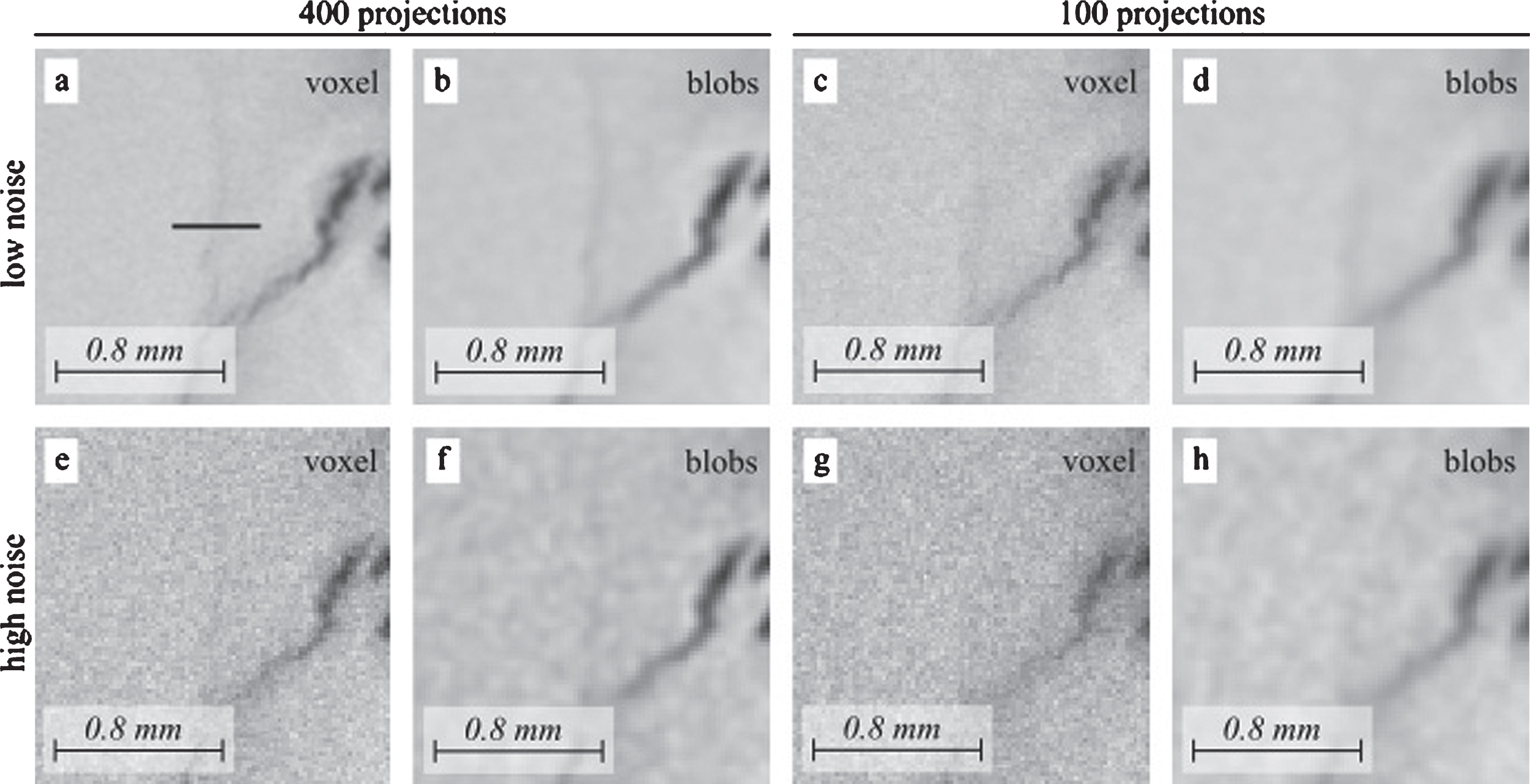
For big cracks we estimated FWHM and slopes at transitions from crack to background as described before. The estimates of 30 FWHM and 60 slope values were used for a statistical analysis. We removed outliers to ensure a normal distribution, which was confirmed with a Shapiro-Wilk test for normality [24] for each analysis. A paired two-tailed t-test was used for evaluating the null hypothesis that mean of voxel based reconstruction and mean of voxelized blob based reconstruction are statistically indistinguishable for both FWHM and slope. A p-value < 0.05 led to rejecting this null hypothesis, which implies that the means are statistically different. For each test, mean and standard deviation for voxels and voxelized blobs, SNR, the degrees of freedom, the t-statistic value, the p-value, and the effect size, which is a quantitative measure of the strength of a statistical claim [25], are reported for FWHM (Table 1) and slope (Table 2).

Table 1

FWHM statistics of up to 30 different line profiles of the big crack. For the reconstruction using voxel basis functions, the number of iterations was six for lownoise400, ten for lownoise100, six for highnoise400, and 15 for highnoise100. For the reconstruction using blob basis functions, results are given after one iteration. Given are: FWHM: mean±standard deviation of FWHM values, SNR: signal-to-noise ratio estimated by (mean of signal / standard deviation of noise), df: the degrees of freedom (number of samples – 1), t-stat: statistic value, p-val: p-value, and r: effect size

dataset	voxels		blobs
	FWHM	SNR	FWHM	SNR	df	t-stat	p-val	r
lownoise400	9.08±1.24	53.3	9.13±1.3	50.8	27	–0.43	0.67	0.08
lownoise100	9.64±0.87	40.1	9.61±0.6	70.7	28	0.43	0.67	0.08
highnoise400	9.24±1.32	18.7	8.58±1.26	31.2	29	9.40	2.6 10^-10	0.87
highnoise100	10.22±1.0	16.1	9.90±0.86	31.0	26	4.27	2.3 10^-4	0.64

Table 2

Slope statistics of up to 60 different edge profiles. Values given analogously to Table 1. Left and right slope of the profile were analyzed separately

	voxels slope	blobs slope	df	t-stat	p-value	r
lownoise400	6.76±1.45	6.95±1.58	55	–1. 28	0.20	0.17
lownoise100	4.14±0.86	8.06±1.64	59	–30.89	<2.2.10^-16	0.97
highnoise400	2.09±0.52	4. 36±1.15	59	–19.65	<2.2.10^-16	0.93
highnoise100	1.34±0.32	3. 29±0.60	59	–29.24	<2.2.10^-16	0.97

Lownoise400 and lownoise100 showed no statistical difference of means for FWHM (p-value 0.67 for both, cf. Table 1). However, means of highnoise400 (p-value 2.6 10^-10) and highnoise100 (p-value 2.3 10^-4) statistically differed with lower FWHM means for the voxelized blob reconstructions. Both also showed effect sizes > 0.6. Furthermore, SNR for lownoise400 was similar for voxel and blob based reconstructions. For lownoise100, highnoise400, and highnoise100, SNR was between 65% and 90% higher for blob based compared to voxel based reconstructions.

Comparing slope means (Table 2), lownoise400 again showed no statistical difference (p-value 0.21). Slope means of lownoise100, highnoise400, and highnoise100 all statistically differed (p-values < 2.2 10^-16) with effect sizes > 0.9, constituting bigger slopes for voxelized blob based reconstructions.

We also examined if a convolution of the voxel based reconstruction with a kernel corresponding to the used blob parameters is able to achieve comparable results. Convolving the highnoise100 voxel based reconstruction with the corresponding blob kernel, the same statistical evaluation was performed as shown above. FWHM values were statistically not different with voxel based values of 10.13±0.84 and blob based values of 10.03±0.74 resulting in a p-value 0.13 and an effect size 0.29. For the slope values, the convolution enhanced results with voxel based values of 1.34±0.3 and convolution based values of 2.58±0.48, which resulted in a p-value < 2.2 10^-16 and an effect size 0.96. However, comparing convolution and blob based reconstruction gave a statistically significant impact with convolution based values of 2.58±0.48 and blob based values of 3.3±0.57 resulting in a p-value < 2.2 10^-16 and an effect size 0.89. This means, that the blob based reconstruction enhanced the convolved reconstruction much further, which experimentally verified that a blob based reconstruction is superior.

Measuring FWHM and slope was not possible for the small crack in a meaningful manner for most setups. Because of this, we analyzed the line profiles with added mean and standard deviations of one, two, and three (Fig. 7). As the images were normalized so that the noise has Gaussian distribution with a mean of 0 and a standard deviation of 1, it is known that 95.45% of the noise has values between – 2 and 2, and 99.73% lie within – 3 to 3. That means a signal is detectable with high probability if it has values bigger than 2 or lower than – 2. Based on that we compared the small crackresults.

Fig.7

Line profiles of the small crack. Dashed line: voxel based reconstruction and solid line: voxelized blob based reconstruction. Additionally, dotted lines for mean (μ) and standard deviations (σ) of one, two, and three are shown. a) lownoise400, b) lownoise100, c) highnoise400, and d) highnoise100. Due to normalization, x- and y-axis have the same spacing (μ= 0, σ= 1).

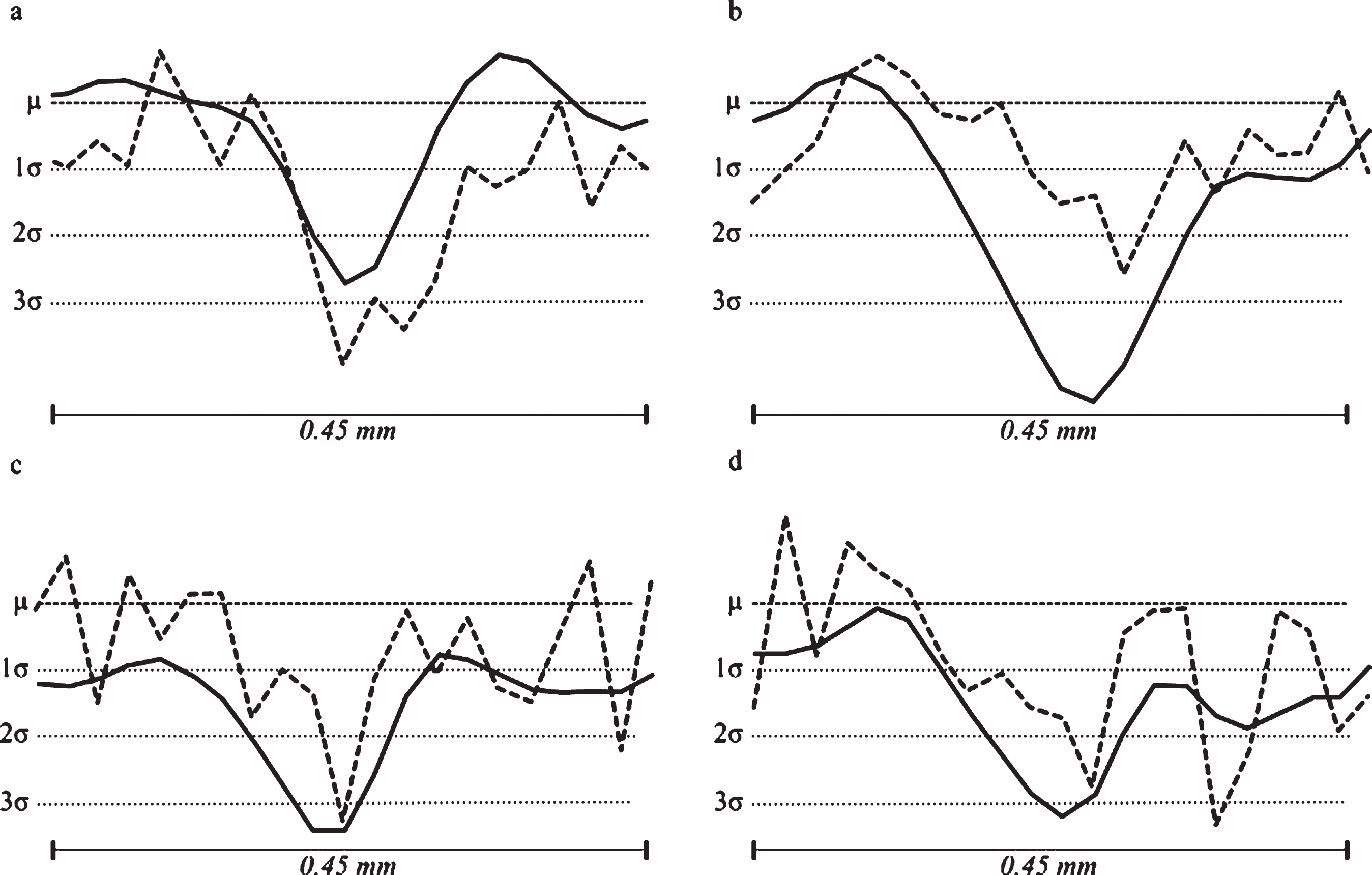
For lownoise400, the small crack was visible in both voxelized blob and voxel based reconstruction. The line profile of the voxels had two minima and values near – 4 that were signal. The blobs had a smoother line profile with only one minimum and lowest value around – 2.5. In this case, FWHM for voxels was bigger with 4.59 compared to voxelized blobs with 3.74. For lownoise100 the voxelized blobs reconstruction looked more blurry, but the small crack was clearer separated from the neighborhood as in the voxels reconstruction (Fig. 7b). The line profile of the voxels had almost no values below two standard deviations, whereas the blobs line profile had several values below, which showed that there is signal.

In the highnoise400 dataset the small crack was visible for voxelized blobs, but hardly for voxels. The line profile of the voxelized blobs was smoother and around the crack several values were large enough to be signal. The values of the voxel line profile were mainly within two standard deviations, and only a single value was below. In the highnoise100 it was similar for voxelized blobs and voxels but with bigger values. Furthermore, the line profile of the voxels had an additional minimum with a lower value than the small crack minimum at a position with only noise, so that noise and signal were indistinguishable. That is the reason that nothing was visible in the voxels reconstruction, but also in the voxelized blobs reconstruction the small crack was hardlyvisible.

3.2Parametrizing blob functions

The basis functions used in our algorithm are specified by three parameters: the smoothness parameter or order m, the radius a, and the shape parameter α. Mathematical arguments suggest that an order of m = 2 should be a good choice, as using this value results in a bell shaped radial profile that decreases smoothly to zero at r = a [12]. The expectation was confirmed experimentally.

The radius a and the shape parameter α specify the support and the bandlimit of the basis functions, respectively. Blobs with a larger radius have a lower bandlimit, i.e. result in a more effective suppression of noise but also blur the reconstruction. We found experimentally that for our dataset, a = 3.0 gives optimal results. However, the desired bandlimit depends on the properties of the dataset. Therefore, we expect this finding to be specific to our dataset and an optimal value for a needs to be determined manually for each situation.

Once the radius a is known, an optimal value for α can be computed using the formula from [13]. For our dataset, α was derived to be ≈11.3. As expected, using this value resulted in best reconstruction quality.

3.3Computational efficiency

Reconstructions were performed on an AMD Radeon R9 390 and on an NVidia GeForce GTX 970, both installed in an Intel Core i7-4790 system running at 3.6 GHz. For the dataset with 400 slices, the runtime on the AMD hardware was 8:38 min (NVidia: 8:43 min) per iteration using voxel basis functions and 1:56:38 (NVidia: 1:54:36) per iteration using blob basis functions. For the dataset with 100 slices, the runtime on the AMD hardware was 1:47 min (NVidia: 1:52 min) using voxel basis functions and 29:21 min (NVidia: 28:51) per iteration using blobs. So overall, using blob basis functions lead to an increased computational demand of a factor of ∼13 - 17 per iteration compared to using voxel basis functions. This increase is caused mainly by the larger support of blob basis functions compared to voxel basis functions, which leads to an increased memory bandwidth consumption. However, the increased computational demand is mostly compensated for by a faster convergence rate. Using the blob basis, optimal results can be achieved after only one iteration of SART, while the voxel basis function requires 6–15 iterations to reach optimal results.

4Discussion

We compared SART reconstructions of laminography datasets using a volume discretization based on (i) voxel basis functions and (ii) based on blob basis functions. Performance was evaluated with varying setups, so that different levels of noise and different numbers of input projections for the reconstruction could be tested. These setups reflected a varying amount of radiation dose, whereby noisier datasets as well as fewer projections constituted less dose. Several parameters and iteration numbers were applied and the best result for each setup was used as input for the evaluation. For each setup, a statistical analysis of line profile properties was conducted. FWHM for 30 line profiles and 60 slopes at transitions from background to signal were estimated. After removing outliers to ensure normality, a paired two-tailed t-test was applied between voxel based and voxelized blob based reconstructions. This statistical analysis in combination with visual inspections was used to judge the capabilities of the two approaches.

Results were influenced by the amount of noise in the input images and the number of projections used for a reconstruction. Lownoise400 showed no statistical difference for both FWHM and slopes, and also SNR values were similar. For lownoise100, there was no statistical difference for FWHM, but slopes indicated a small but statistically significant advantage for the blob reconstruction, also confirmed by SNR values. Visual inspection of the results did not reveal a clear advantage for either method. The voxelized blob reconstruction looked smoother in both cases but also less sharp, so the overall impression was ambiguous. That means, for perfect datasets with little to no noise, none of the methods was superior.

For noisy datasets, however, blob basis functions showed a benefit over voxel basis functions, particularly if only a small number of projections was available. In highnoise400 and highnoise100, blob based reconstructions showed superior quality both quantitatively in terms of FWHM, slopes and SNR and by subjective inspection. Voxel based reconstructions were much noisier, which made it hard to identify visually the exact locations of transitions from background to signal. In addition, the small crack was hardly visible in highnoise400 and not visible in highnoise100. In contrast, voxelized blob based reconstructions separated background and signal clearer, which was supported by the better visibility of the small crack in highnoise400. For highnoise100 it was harder to judge, but at least a signal different from the background was visible. This showed, that blob based reconstructions can enhance prominent structures, but may not help with small structures, especially when only few projections with too low dose are given.

For data with little to no noise and a sufficient number of projections in the sense of the Crowther criterion [26], results were different from voxel based reconstructions, but with no clear preference for either method. That means blob based reconstructions should be used for laminography datasets in cases where incomplete or noisy data can be expected.

5Conclusion

We have presented a blob based reconstruction scheme for laminography datasets. A voxel based approach has been implemented within the same framework to be able to demonstrate the benefits of using blobs. A laminography dataset was evaluated with different setups from a low level of noise to a high level and from a small number of projections to a larger number. We found that if the number of projections fulfills the Crowther criterion and the amount of noise is small compared to the signal strength, both choices of basis functions provide results of identical quality. In the presence of a high level of noise compared to the signal and with a smaller number of input projections that does not fulfill the Crowther criterion, using blobs as basis functions resulted in superior reconstruction quality, which was assessed quantitatively using FWHM, slopes of edge profiles, and SNR.

Taking these results it is recommendable to use blobs as basis function for laminography datasets, as they deliver equal or better results than voxels in terms of resolution and sharpness. A higher resolution facilitates the interpretation of reconstructed datasets as it is easier to identify structures when applying blob based reconstructions. Furthermore, this enhancement may make it possible to acquire datasets using less dose that, nevertheless, achieve a comparable resolution to higher dose datasets (i) by using less dose for a single projection, which leads to more noise, or (ii) by reducing the number of projections.

Acknowledgments

The work of the authors was supported by Deutsche Forschungsgemeinschaft under grant LO 310/13-1, MA 5836/1-1 and SL 38/5-1 within the DFG grant IMCL. The authors thank the DFKI GmbH for additional funding and for providing the necessary infrastructure.

References

[1]	Zhou J. , Maisl M. , Reiter H. and Arnold W. , Computed laminography for materials testing, Appl Phys Lett 68: (24) ((1996) ), 3500.
[2]	Maisl M. , Porsch F. and Schorr C. , Computed Laminography for X-ray Inspection of Lightweight Constructions, in 2nd International Symposium on NDT in Aerospace, (2010) , pp. 2–8.
[3]	Gondrom S. , Zhou J. , Maisl M. , Reiter H. , Kröning M. and Arnold W. , X-ray computed laminography: An approach of computed tomography for applications with limited access, Nucl Eng Des 190: (1–2) ((1999) ), 141–147.
[4]	Helfen L. , Xu F. , Suhonen H. , Urbanelli L. , Cloetens P. and Baumbach T. , Nano-laminography for three-dimensional high-resolution imaging of flat specimens, J Instrum 8: (5) ((2013) ), C05006–C05006.
[5]	Helfen L. , Baumbach T. , Pernot P. , Mikulík P. , DiMichiel M. and Baruchel J. , High-resolution three-dimensional imaging by synchrotron-radiation computed laminography, Proc SPIE 6318: ((2006) ), 63180N.
[6]	Helfen L. , Xu F. , Suhonen H. , Cloetens P. and Baumbach T. , Laminographic imaging using synchrotron radiation – challenges and opportunities, J Phys Conf Ser 425: (19) ((2013) ), 192025.
[7]	Maisl M. , Marsalek L. , Schorr C. and Horacek J. , GPU-accelerated Computed Laminography with Application to Non-destructive Testing, in 11th European Conference on Non-Destructive Testing (ECNDT) (11: ) ((2014) ), 329.
[8]	Grant D.G. , TOMOSYNTHESIS: A Three-Dimensional Radiographic Imaging Technique, IEEE Trans Biomed Eng BME-19: (1) ((1972) ), 20–28.
[9]	Herman G.T. , Lent A. and Rowland S.W. , ART: Mathematics and applications, J Theor Biol 42: (1) ((1973) ), 1–32.
[10]	Andersen A.H. and Kak A.C. , Simultaneous algebraic reconstruction technique (SART): A superior implementation of the art algorithm, Ultrason Imaging 6: (1) ((1984) ), 81–94.
[11]	Lewitt R.M. , Multidimensional digital image representations using generalized Kaiser–Bessel window functions, J Opt Soc Am A 7: (10) ((1990) ), 1834.
[12]	Lewitt R.M. , Alternatives to voxels for image representation in iterative reconstruction algorithms, Phys Med Biol 37: (3) ((1992) ), 705–716.
[13]	Matej S. and Lewitt R.M. , Practical Considerations for 3-D Image Reconstruction Using Spherical Symmetric Volume Elements, IEEE Trans Med Imaging 15: (1) ((1996) ), 68–78.
[14]	Garduño E. and Herman G.T. , Optimization of basis functions for both reconstruction and visualization, Discret Appl Math 139: (1) ((2004) ), 95–111.
[15]	Popescu L.M. and Lewitt R.M. , Ray tracing through a grid of blobs, in IEEE Symposium Conference Record Nuclear Science 2004 6: (C) ((2004) ), 3983–3986.
[16]	Marabini R. , Herman G.T. and Carazo J.M. , 3D reconstruction in electron microscopy using ART with smooth spherically symmetric volume elements (blobs), Ultramicroscopy 72: (1–2) ((1998) ), 53–65.
[17]	Bilbao-Castro J.R. , Marabini R. , Sorzano C.O.S. , García I. , Carazo J.M. and Fernandez J.J. , Exploiting desktop supercomputing for three-dimensional electron microscopy reconstructions using ART with blobs, J Struct Biol 165: (1) ((2009) ), 19–26.
[18]	O’brien N.S. , Boardman R.P. , Sinclair I. and Blumensath T. , Recent Advances in X-ray Cone-beam Computed Laminography, J Xray Sci Technol 24: (5) ((2016) ), 691–707.
[19]	Dahmen T. , Marsalek L. , Marniok N. , Turoňová B. , Bogachev S. , Trampert P. , Nickels S. and Slusallek P. , The Ettention software package, Ultramicroscopy 161: ((2016) ), 110–118.
[20]	Vogelgesang J. and Schorr C. , A Semi-Discrete Landweber–Kaczmarz Method for Cone Beam Tomography and Laminography Exploiting Geometric Prior Information, Sens Imaging 17: (1) ((2016) ), 17.
[21]	Bresenham J.E. , Algorithm for computer control of a digital plotter, IBM Syst J 4: (1) ((1965) ), 25–30.
[22]	Dahmen T. , Baudoin J.-P. , Lupini A.R. , Kübel C. , Slusallek P. and De Jonge N. , Combined scanning transmission electron microscopy tilt- and focal series, Microsc Microanal 20: (2), ((2014) ), 548–60.
[23]	Rieger B. and van Veen G.N.A. , Method to determine image sharpness and resolution in Scanning Electron Microscopy images, in EMC 2008 14th European Microscopy Congress 1–5 September 2008, Aachen, Germany, vol. 1: , Berlin, Heidelberg: Springer Berlin Heidelberg, (2008) , pp. 613–614.
[24]	Shapiro S.S. and Wilk M.B. , An analysis of variance test for normality (complete samples), Biometrika 52: (3–4) ((1965) ), 591–611.
[25]	Rosenthal R. and DiMatteo M.R. , Meta-Analysis: Recent Developments in Quantitative Methods for Literature Reviews, Annu Rev Psychol 52: (1) ((2001) ), 59–82.
[26]	Crowther R.A. , DeRosier D.J. and Klug A. , The Reconstruction of a Three-Dimensional Structure from Projections and its Application to Electron Microscopy, Proc R Soc London Ser A, Math Phys Sci 317: ((1970) ), 319–340.