
A weighted plus/minus metric for individual soccer player performance
Abstract
Despite soccer being the number one sport in the world in many respects, the “beautiful game” still lags behind other sports in terms of analytics. We propose a weighted plus/minus metric to be used as an instrument to evaluate player performance. An unweighted plus/minus metric subtracts goals conceded from goals scored for each player while on the field of play and are regularly used in hockey or basketball. Key improvements to this established, unweighted +/– metric include control for opponents’ strength, the importance of a particular goal, and considerations for the fact that scoring is less frequent in soccer. The results from three teams (Bayern Munich, VfL Wolfsburg, Werder Bremen) in the German Bundesliga from the 2012-13 season were used as a demonstration and comparison of the two metrics. In addition to the creation of a weighted +/– system, a spatial mapping system of team shots was developed to give a potential visual explanation of why certain players were a net positive/negative influence for their team.
1Introduction
As analytics continue to grow in nearly all sports, it is surprising that soccer, the number one sport in the world, lags behind. Although soccer analytics are an emerging field, they have not yet reached the levels to which baseball or basketball have assimilated such analysis on the level of Sabermetrics (James, 1982) or Goldsberry’s Courtvision (Goldsberry, 2012). We introduce a +/– system to evaluate player performance, a task considered to be difficult due to the game’s complex nature. In one example, a team’s success may be linked to a certain player’s performance over the course of a season. The +/– system would show whether a player’s presence on the field is a net positive or negative for his team, regardless of position. It allows for the comparison of a player’s net influence on team performance with other teammates. This approach is a significant advancement in statistics in the field of soccer beyond basic statistics such as goals, assists or tackles. As such, the +/– system adds a quantitative insight into a player’s performance which could improve coaches’ and manager’s decisions both in the training and scouting realms of the game. It also extends +/– metrics in other sports in two ways: (1) by controlling for the importance of goals (a go-ahead goal, for instance, should be more valuable than a goal that makes it 5-0) and (2) by controlling for opponents’ strength (scoring against a heavy favorite is harder than against a weak opponent). Examples of positive and negative influences will be displayed in the results and discussion sections of the paper.
Analytics in soccer have been utilized before, but typically in a more general theme. Anderson and Sally’s 2013 book examined statistics on a large scale by responding to questions like “does possession matter?” and asks questions such as what role total team salaries or coaches have on a team’s success (Anderson & Sally, 2013). It also summarized several other papers from previous decades starting with Britain’s Charles Reep in the middle of the 20th Century (Reep & Benjamin, 1968). In terms of more recent research, there have been advances from Ian McHale, where in 2007, McHale and Scarf developed a match prediction model, and in McHale et al. (2012), a player evaluation system was developed for the Barclay’s Premier League using several sub-indices. While that approach uses a variety of individual player performance data (such as goals scored, shots, assists, clean sheets), the +/– metric we introduce focuses on the one most crucial team performance measure – goals – and uses it to determine individual contribution to team success. From a team perspective, Oberstone (2009) performed regression analysis on team’s actual vs. model predicted season success rates in the Barclay’s Premier League. The 2014 Sloan Sports Analytics conference, the United States’ foremost meeting on sports analytics, featured one paper on formation analysis that confirmed the old adage that teams play for the draw on the road and play for the win at home (Bialkowski et al., 2014).
We also introduce a spatial mapping system of events to visualize the “how” and “why” a player’s net influence is positive or negative. In terms of spatial analysis in soccer, there has been very little literature on the matter. There have been studies on the spatiality of socio-economic impacts of soccer (Forrest et al., 2002) and studies on media and spatial events in soccer (Yow et al., 1995; Ekin, 2003). In terms of specific spatial statistics of events on the pitch, studies have been limited in scope (Kim et al., 2011). McHale and Szczepański (2014) performed a statistical and spatial based mixed effect model for predicting goal scorer success. However, this paper was focused more on direct prediction of events. It only addresses goal scoring ability of footballers, which without a doubt is an important skill, but leaves out other important features such as the avoidance of goals against. By using quantitative methods that are backed up by spatial visualizations to evaluate player performance, one can understand a player’s net effect on a team’s success.
We first summarize the methods behind the creation of the +/– metric, in which the justification and mathematics will be presented. This is followed by a section including the results of the plus-minus metric for the case studies used in this paper. We then present a discussion of the results, including visualizations of potential reasons why certain players are net positives or negatives on their teams. This is followed by a brief conclusion considering the implications of advanced analytics in soccer. The main objective of this paper is to display the utility of the +/– metric, highlighting three teams (Bayern Munich, VfL Wolfsburg and Werder Bremen) with very different end season outcomes in the 2012-13 German Bundesliga season.
2Methodology
Plus/minus metrics are well established, especially in hockey (Macdonald, 2011), but are also used to evaluate player performance in other team sports, e.g. basketball (Sill, 2010). The idea is simple: whenever the team scores, all players on the court at the time of the event receive positive points. Whenever the team is scored against, the players who are currently playing receive negative points. Combining the negative and positive values over time yields the “plus/minus” statistic. Consequently, players who have positive scores in this metric were on the court when the team performed well (scored more often than the opponents), while players with negative values were on the court when their team was outscored by the opponents. The plus/minus metric implicitly assumes that all players on the pitch/court contribute to the team’s success to the same extent. In sports with frequent formation changes, this metric can also be interpreted as an individual player’s contribution to the team’s success.
The simplest version of the metric (subtracting points/goals against from points/goals for) also treats all scoring events equally. A strong objection against this assumption is that scores in already decided games (in “garbage time”) are less valuable than scores in tight games or in “crunch time”. Another objection is that winning against weak opponents is not as valuable as winning (or tying) against heavy favorites. The simple version of the plus/minus metric does not account for either of the two concerns.
While in-game formation changes are not as frequent in soccer as they are in hockey or basketball (mainly because substitutions are limited to three per game), they do occur more often between games due to injuries, suspensions, and coach’s decisions. Scoring events also occur less frequently in soccer, but often enough to assume acceptable levels of statistical validity (around 100 events per team per season on average). What makes this plus/minus metric unique is that it addresses the two objections mentioned above by controlling for goal importance and for relative opponent’s strength. The +/– metric for Player x for the entire season is calculated with the following formula:
(1)
Equation 1. Calculation of weighted plus/minus metric in the B-FASST system.
The variable w stands for the week of the game (the season has W weeks), t stands for the minute in the games (T is the total number of minutes for each game). This means that the calculation takes place on a per-minute basis. Summing up over all minutes in all games then yields the plus/minus score. The variable wp stands for “winning probability” according to the betting quotas of Bet365, a frequently used source for evaluating team strengths in econometrics (e.g. Franck et al., 2011). We subtract the player’s team’s winning probability from the opponent’s winning probability to obtain the number of points that each player obtains if the game ended in a draw and if the player played the entire game. Dividing this number by the number of minutes the game lasted (90–95), yields a per-minute value.
For instance, when Bayern Munich played Schalke 04, betting a dollar on a Bayern win would yield 1.91 dollars in the winning case. By taking the reciprocal value of the quota, this translates into an expected winning probability for Bayern of 52% (wpown = 0.52). Schalke’s quota was 4.0, translating into wpopp = 0.25. Accordingly, all Bayern players would receive –0.27 points if the game ended in a draw (Schalke players would get the positive equivalent). Note that the probabilities do not add up to 1, mainly because we do not need to consider draws here. Subtracting the two winning probabilities should also eliminate large parts of the bookmakers’ markups (bookmakers worsen quotas in their favor which allows them to make profits). The first part of the equation therefore controls for relative strengths of the opposing teams in each game.
We assume that betting quotas from professional betting agencies are a good way to capture relative strengths of the opposing teams, because this source is expected to have a very high information level about each match, incorporating not only quantitative data from previous matches, but also qualitative information, e.g. about injured players or special events that happened recently that might affect the game. There has been quite extensive research on the effectiveness of league football betting markets in the sense that betting odds reflect the available information (e.g. Croxson & Reade, 2014; Deschamps & Gergaud, 2007; Dobson & Goddard, 2011; Forrest et al., 2005; Goddard, 2005; Goddard & Asimakopoulos, 2004; Spann & Skiera, 2009) and consequently on the quality of the information when using betting quotas as a proxy for team strength. While there is evidence that bookmakers possibly try to exploit behavioral biases of bettors, e.g. a “sentiment bias” leading to worse quotas for popular teams (Braun & Kvasnicka, 2013; Forrest & Simmons, 2002), the overall picture tends to support high degrees of efficiency in the market (Croxson & Reade, 2014; Simmons, 2013; Spann & Skiera, 2009). Betting odds for weekend games are collected Friday afternoons, and on Tuesday afternoons for midweek games.
The second part of the equation accounts for the importance of goals. Subtracting the goal differential in a particular game one minute before the actual minute from the goal differential in the actual minute (Δgoalst,w - Δgoalst-1,w) yields “1” if the player’s team scored, “0” if no one scored, and “–1” if the opponent scored in the current minute. This part therefore determines whether scored goals count in favor or against the considered player. Most importantly, the following fraction takes the value of “1” if the goal is “point relevant”, meaning that the goal changes the outcome of the game from any of the three possible fundamental outcomes (win, draw, loss) to another. A goal that consolidates to an existing outcome (win or loss) is then only worth 1/2, 1/3, 1/4 and so on, depending on how large the goal differential already is. The last part
While the “goals part” of the equation supports players of teams that outscore their opponents, the “winning probability” part integrates a priori expectations into the metric. Favorites effectively start out with a burden, so to say. If the a priori favorites fail to outscore the underdog, its players will end up with a negative +/– score for that match, because they failed expectations. Players on the underdog team, however, receive positive scores due to the fact that they outperformed expectations. Consequently, a team that exceeds expectations should have most players in the positive while teams that underperform relative to expectations should have most players with a negative plus/minus value. A team that approximately meets expectations should have players with values around zero.
3Results
For the following tables, all relevant game data (goals, goal time, player minutes logged, lineups, player substitutions, and yellow and red cards) were collected from ESPNFC.com’s game reports. To illustrate how the metric works, Table 1 presents plus/minus metrics for frequent starters of the following three teams: Bayern Munich (a team that played a historically great season, winning the Bundesliga with a new point record as well as the domestic cup and the UEFA Champions League), VfL Wolfsburg (a team that ended up in the middle of the table and approximately met a priori expectations), and Werder Bremen which failed expectations greatly and barely avoided relegation. The results validate our expectations: even after correcting for relative team strengths, Bayern players score very high values in general (reflecting their dominance), while Werder players score low values. Wolfsburg’s values approximately revolve around zero.
Table 1
Plus/minus statistics and net team shots per 90 minutes
| Player | A1 | B1 | C1 | Player | A2 | B2 | C2 | Player | A3 | B3 | C3 |
| Neuer | 74 | 24.24 | 8.71 | Polak | 9 | 8.37 | 0.97 | Elia | –1 | 0.11 | 3.87 |
| Lahm | 69 | 22.97 | 9.72 | Hasebe | 7 | 5.41 | –1.39 | Arnautovic | –7 | –3.46 | 1.54 |
| Dante | 69 | 22.68 | 8.92 | Kjaer | 5 | 4.24 | –2.09 | Bargfrede | –4 | –4.57 | 1.89 |
| Ribery | 61 | 21.60 | 9.82 | Olic | 1 | 3.03 | –0.28 | Ignjovski | –9 | –4.81 | 4.09 |
| Schweinsteiger | 57 | 18.33 | 9.61 | Diego | –2 | 2.30 | –1.36 | Petersen | –9 | –6.18 | 3.76 |
| Boateng J | 59 | 18.28 | 9.87 | Träsch | 2 | 0.84 | 1.34 | Sokratis | –9 | –6.49 | 2.92 |
| Martinez | 49 | 16.68 | 8.21 | Benaglio | –5 | 0.10 | –1.03 | Lukimya | –8 | –7.51 | 4.31 |
| Müller T | 48 | 16.08 | 9.23 | Dost | –4 | –0.08 | –1.59 | Junuzovic | –13 | –7.85 | 3.43 |
| Kroos | 47 | 14.16 | 9.81 | Vieierinha | –4 | –0.78 | 1.14 | Hunt | –13 | –8.07 | 3.01 |
| Mandzukic | 38 | 13.10 | 10.54 | Naldo | –7 | –1.53 | –0.79 | Fritz | –13 | –8.29 | –0.16 |
| Gustavo | 43 | 13.06 | 8.37 | Rodriguez | –6 | –1.72 | –0.15 | G. Selassie | –17 | –9.60 | 2.3 |
| Alaba | 41 | 12.33 | 7.43 | Josue | –4 | –2.29 | –4.2 | De Bruyne | –15 | –9.75 | 2.88 |
| Robben | 33 | 11.87 | 8.73 | Fagner | –9 | –2.92 | –1.45 | Mielitz | –16 | –10.21 | 2.9 |
| Badstuber | 30 | 9.98 | 11.42 | Schäfer | –7 | –3.34 | –2.26 | Prödl | –15 | –10.64 | 1.23 |
| TEAM AVG | 36.7 | 11.96 | TEAM | –1.79 | 0.11 | TEAM | –7.2 | –4.66 |
Unweighted plus/minus values (A), Weighted plus/minus values (B) and net team shots per 90 minutes (C) for selected team players in the 2012-13 Bungesliga Season on Bayern Munich (1st place, 91 points, League Champions, +80 goal differential (GD)), VfL Wolfsburg (11th Place, 43 points, –5 GD) and Werder Bremen (14th place, 34 points, 3 points above potential Relegation, –16 GD).
An unweighted +/– metric, similar to what is used in the National Hockey League or National Basketball Association, (Table 1, column A) was also calculated to display the differences with the weighted +/– metric proposed in this paper (Table 1, column B). The results are similar in that they find an approximate agreement with the rank order of individual players. For example, Bayern Munich (Columns A1 and B1) players Manuel Neuer, Philip Lahm and Dante are ranked numbers 1, 2, and 3 for both systems. This trend continues in a fairly consistent manner as one examines the roster for players with lower scores. This also happens when viewing the VfL Wolfsburg (Columns A2 and B2) and Werder Bremen (Columns A3 and B3) rosters. However, there are differences that make the weighted +/– score an improvement over the unweighted +/– score.
In one such example, Werder Bremen had three players end the season with an unweighted +/– score of – 13: Zlatko Junuzovic, Aaron Hunt, and Clemens Fritz. If an unweighted +/– system were utilized as a means of analysis for player performance, one would have to assume that the three players contributed exactly the same level of performance. The weighted +/– system proposed in this paper, by adjusting for the weaknesses found in a traditional unweighted +/–, finds that the players did not contribute the same levels of performance. While the three were still given negative scores, the players gave different levels of performance based on the importance of the goals scored when they were on the playing field. Similarly, Theodor Gebre Selassie was given an unweighted score of – 17, ranking him last on the Werder Bremen roster. However, the weighted +/– system found that Gebre Selassie finished comparatively higher on the roster with a score of – 9.60, and that Sebastian Prödl (unweighted: – 15, weighted: – 10.64) should have been considered to have had the lowest performance score. VfL Wolfsburg’s roster displays similar results in terms of disagreement. Some players (Diego, Benaglio) register a negative unweighted score along with a positive weighted score.
For a team who achieved historic success, Franck Ribéry, also the 2012/2013 UEFA Best Player in Europe, proves to be one of Bayern’s key players according to the metric. The weighted plus/minus metric also identifies Wolfsburg’s Jan Polak as the team’s key player, clearly ahead of the club’s stars Diego and Ivica Olic. For Werder Bremen, it is striking that the team’s captain, Clemens Fritz, reveals a particularly poor plus/minus score, not only in absolute terms, but also relative to his teammates.
The results might lead to the impression that the metric strictly favors players from winning teams. However, this is mainly due to our selection of teams. Since the metric adjusts for relative team strengths, players do not benefit from winning alone, but rather from exceeding a priori expectations. It is therefore possible that players from teams that finish lower in the table than another team still outperform players from the latter team, as long as the “weaker” team outperformed expectation to a larger extent than the better placed team.
4Spatial analysis of weighted plus/minus values
The plus/minus metric can help identify players’ contributions to the team’s overall success during the course of several games or an entire season and find explanations for players’ good or bad performances. The metric is objective and can be used by a team to find which players are contributing most positively and negatively to a team’s effort. Of course, the same metric can be used by opposing teams to find which players to focus on in an upcoming match. Another possible application is inter-team comparison which potentially improves a manager’s decisions when compiling rosters. This shows that the plus/minus metric has a dual nature, as it can be used both as an evaluation tool for one team and a scouting tool for another. For example, the results from Wolfburg’s plus/minus ratings for the 2012-13 Bundesliga season (Table 1) shows that Jan Polak controls Wolfsburg’s success to a larger extent than Diego or Olic, the team’s most recognized players. An opposing manager not employing this weighted plus/minus system might not be able to understand the players who are the most critical for an opponent’s success and create tactics based on a general strategy. A manager with the weighted plus/minus system might direct his players to pay more attention to a holding midfielder like Jan Polak (+8.37) or Bayern’s Bastian Schweinsteiger (+18.33) who seems to control the flow of offense more than it appears, rather than the potentially explosive attacking midfielder/striker Arjen Robben (+11.87). Doing so might cut off dangerous through balls to Robben, preventing the Dutch national from getting chances in the attacking third.
One method to reinforce the results of the +/– system is to visualize potential reasons for why a certain player was a net positive or net negative influence on his team’s success. Skill, strategy and luck all combine to create the flow of the game for each team, and as the game progresses, a multitude of events occur on the pitch. Runs up the left flank, early crosses to a center forward making a run, missed challenges just outside the 18-yard box, diving saves to keep a shot out of the goal; all are actions that occur on the pitch and are the sum of a number of smaller, individual events. These individual events can all be tracked, mapped and analyzed to look at soccer with more depth than ever before. While there are some companies who record all events (Opta, Impire), we chose to utilize shot location data in this study. Location of shots figured/conceded is not a perfect gauge of a team’s achievement, but it is a good relative indicator of team success on offense and defense (Rampinini et al., 2009; Collet, 2013).
We primarily employed game summaries from ESPNFC.com, and manually entered the shot location in a Geographic Information System: ESRI’s ArcGIS version 10. Each shot was logged and assigned different values in the fields of “Game Number, Opponent, Time, Shot Taker, Shot Result and Shot Type (when available).” Once all shot location was logged, the data were summed up in 2×2 meter cells that make up a grid that covered the entire field, creating a grid populated with the total shots figured over the given amount of time. Each grid cell was represented by its centroid. After each grid centroid point value (total shots) was calculated, the values were interpolated to create a continuous field of data. The Inverse Distance Weighting (IDW) methodology of spatial interpolation was used, with a decay variable of 1.333 and 24 “nearest neighbor” points for each grid cell. IDW was chosen because the authors feel that this methodology best represents a continuous field of random, non-equally distributed independent events and is appropriate for events on a sporting field rather than another spatial interpolation method such as kriging. The methodology behind the creation of IDW can be found in Shepard (1968) and a review differentiating the capacities of IDW versus Kriging can be found in Zimmerman et al. (1999).
The resulting maps were then validated by randomly taking out one shot and determining the root mean square error of the difference between the point with and without the shot. This was done twenty times for each map and a mean absolute error of 0.043 was calculated at each shot location. Such a low value suggests that the dataset was robust enough for spatial analysis and for conclusions to be drawn on the results. On an individual player level, the player’s presence on or off the field was standardized to 90 minutes, to accurately obtain a “per 90 minutes” map. This was necessary in order to account for the fact that some players spend far more time on the field than off and vice versa. If ignored, a systemic bias would be present if a studied player was on the field more than off, leading to more shots being conceded/figured, thus skewing the results.
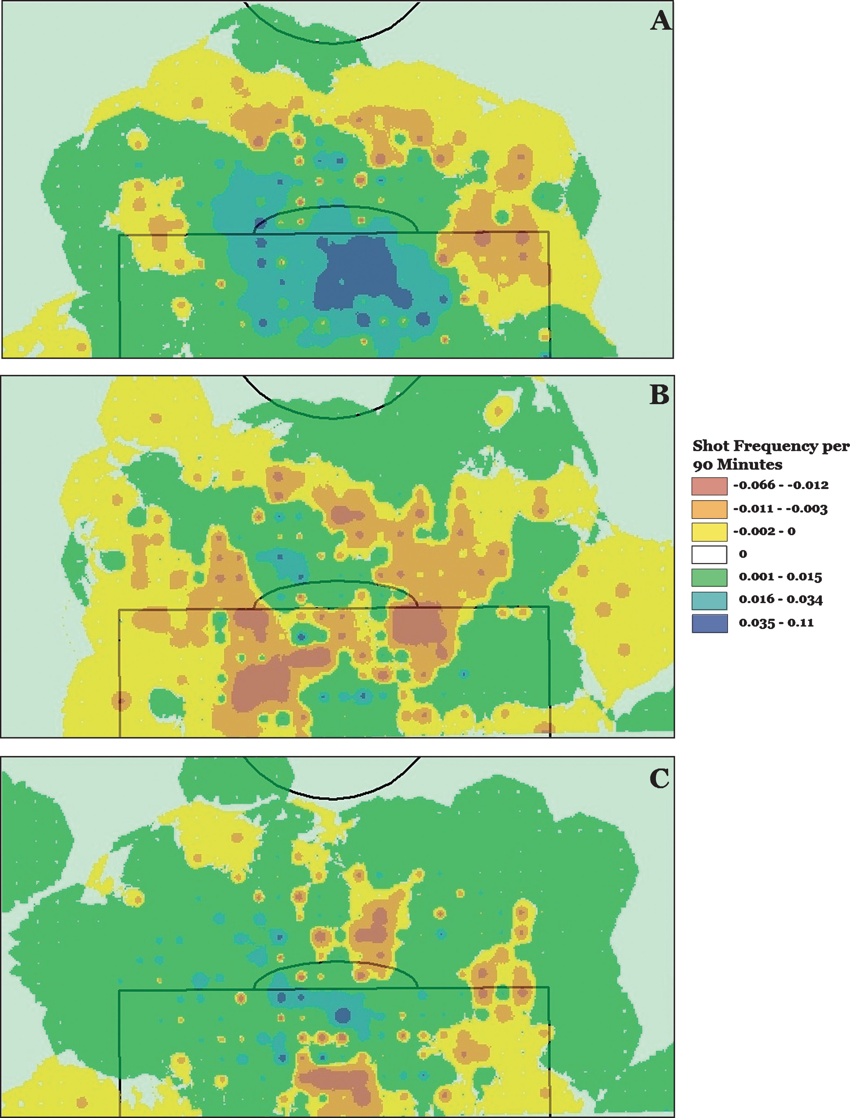
Bayern Munich dominated the European soccer landscape in the 2012-13 campaign winning all competitions they entered. Table 1, Column B1 shows that Bayern’s players are universally positive, but certain players were more of a positive than others. The map (Fig. 1A) shows a team that commanded possession of the ball and took nearly 200 more shots than they conceded, many of them at close range inside the 18-yard box. VfL Wolfsburg met a priori expectations in the 2012-13 season by finishing in the middle of the Bundesliga table. Large investments in stars Diego and Ivica Olic were positive for Wolfsburg, but defensive midfielder Jan Polak was clearly the biggest positive influence (Table 1, Column B2). Wolfsburg’s counterattacking style shows up in the map where, as planned, they surrendered more shots than they took (Fig. 1B). This strategy draws an opponent further up the field looking for a goal, only to be hit back with an odd-man counterattack. It was a difficult season for Werder Bremen, who came into the season with high expectations and barely survived a relegation battle. “Die Werderaner” had some punch on offense (Table 1, Column C3), but a leaky defense cost them dearly. The map shows Werder’s biggest problem: numerous ineffectual shots from distance on offense with regular mistakes on defense leading to chances surrendered at close range (Fig. 1C). Despite a number of personnel changes and tactical switches, Werder’s Head Coach, Thomas Schaaf, was fired just before the end of the season.
Fig.1
Net shot distributions for each team (Panel A: Bayern Munich, Panel B: VfL Wolfsburg, Panel C: Werder Bremen) which were calculated as the spatial distribution of shots taken minus the spatial distribution of shots conceded. Blue/Green colors represent areas where more shots taken than conceded and Orange/Red represent areas where more shots are conceded than taken.
In examining Tables 1 and 2, a player such as Clemens Fritz on Werder Bremen may stand out. Fritz was Werder’s captain for the 2012-13 year, and despite public ridicule of his play he continued to play well into the season. His – 8.29 rating shows that Fritz was a liability when on the field, and Fig. 2 illustrates this fact.
Fig.2
Clemens Fritz Shots conceded. Red/Orange are areas where more shots are conceded when Fritz is on the pitch Green/Blue are areas where more shots are conceded when Fritz is off the pitch.
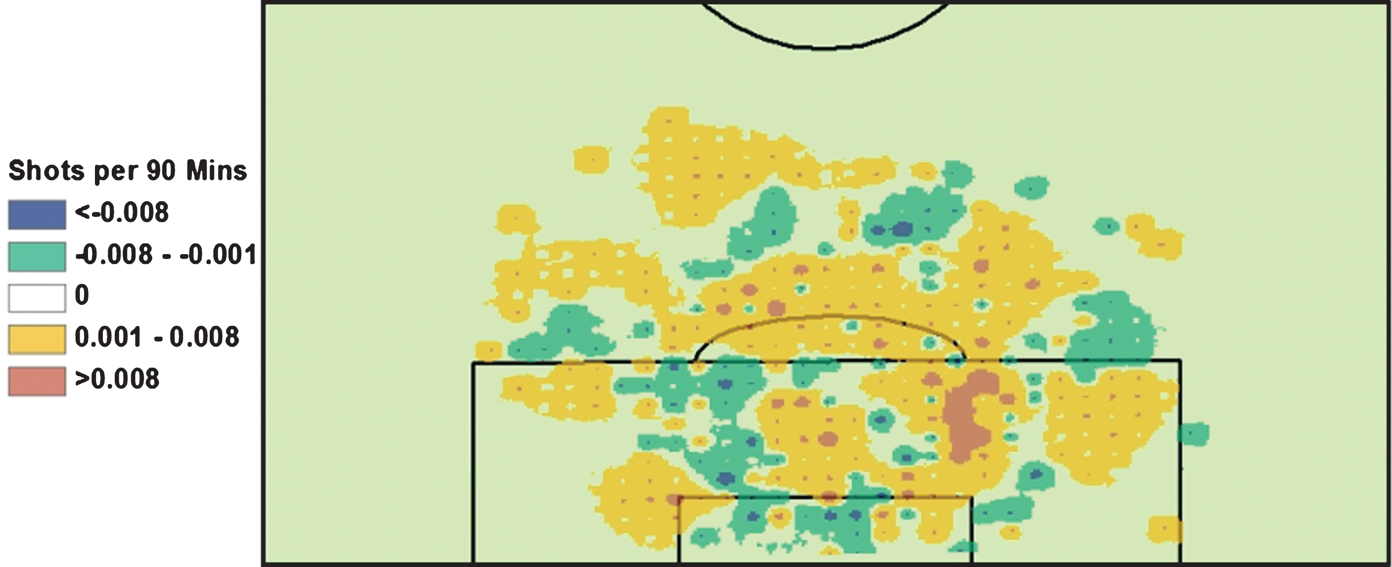
Fig. 2 displays the difference between shots taken when Fritz is on the field minus shots taken when Clemens Fritz is off the field (per 90 minutes). It is very clear that areas within the 18 yard box, to the right side of the field are areas that are more likely to see more shots when Fritz is on the field. That area is the primary location of Clemens Fritz’s position, leading to the conclusion that opposing offenses clearly targeted Fritz’s position on the field because he was a defensive liability (Fig. 2).
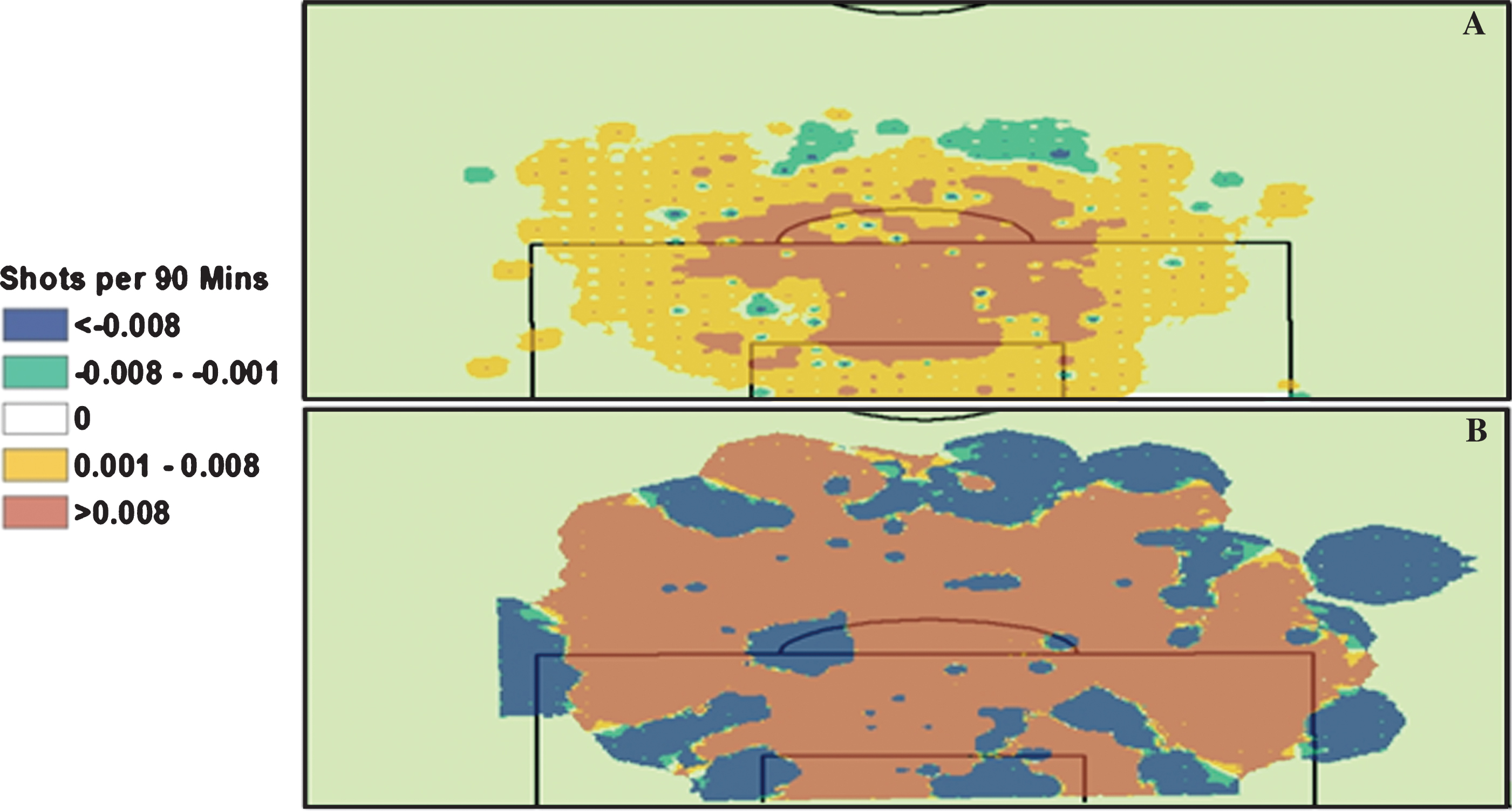
In Fig. 3, we show an individual player’s impact on his team’s performance by focusing on Franck Ribéry, the winner of the 2012/13 UEFA Best Player in Europe Award. Ribéry’s +/– score of +21.60 is higher than any non-goalkeeper or defender on Bayern Munich. He was the best offensive player on the best team in Europe in the 2012-13 campaign. The figure visualizes this by displaying the differences in shots taken (A) and shots conceded (B) when Ribéry is on and off the field (the ratio of his on vs. off field time is approximately 2 : 1). In panel A, one can easily see his impact on the offense, particularly with regards to shots taken in the center of the 18 yard box and on the right wing (the attacking team’s left wing, Ribéry’s position). Panel B illustrates that there are two strong patterns in Ribéry’s presence on or off the pitch, as the maps show areas of far more or far less shots surrendered, rather than small differences like when he is on offense. This suggests that his presence on the field makes Bayern’s defense radically different than when he is off. The +/– system confirms that Ribéry is a very large net positive on his team and the maps demonstrate his game changing ability on both offense and defense (Fig. 3).
Fig.3
Franck Ribéry Shots taken (panel A) and conceded (panel B) In Panel A, Red/Orange are areas where more shots are taken when Franck Ribery is on the pitch. In Panel B, Red/Orange are areas where more shots are conceded when Franck Ribery is off the pitch.
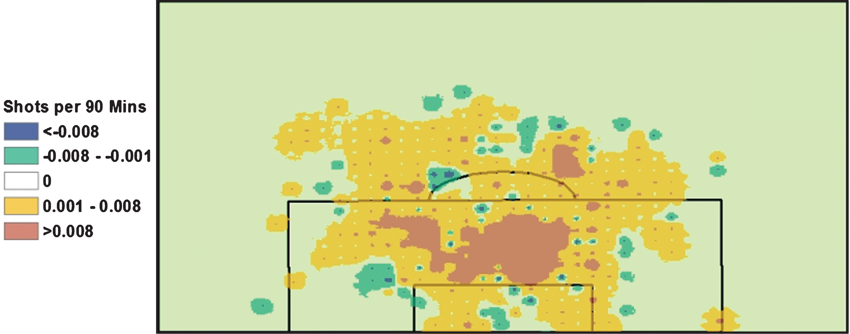
Additionally, we would like to illustrate how we may be able to test hypotheses. While there is no doubt Franck Ribéry is a world class player, it had been hypothesized in the mass media that his brilliance is a function of having an outstanding, but far less heralded player backing him up: David Alaba (+12.33 score), left defensive back for Bayern Munich. Fig. 4 shows that Alaba’s presence leads to more shots on offense, as when Alaba and Ribéry are present, more shots are taken by Bayern Munich compared to when it is solely Ribéry on the field, especially inside the 18-yard box. This suggests that Alaba is important not only for Bayern’s success, but for Ribéry’s success in particular.
Fig.4
Ribéry/Alaba vs. Ribéry only Shots taken. Red/Orange are areas where more shots are taken when David Alaba is on the pitch in support of Franck Ribery. Green/Blue are areas where more shots are taken when Franck Ribery does not have David Alaba in support.
5Conclusion
The sport of soccer is years behind other sports such as baseball and basketball in terms of advanced statistical analytics. There have been some advances on a team level, but overall, the impact of analytics on the game has been minimal – especially in the Bundesliga – as only a few enterprising teams have invested in analytics. This may be due to a lack of commitment, funding or just a refusal to change from “traditional” methods, as seen in other sports. However, in the age of big data, we feel that soccer will soon undergo a “statistical revolution” on the order of some other major team sports as the magnitude of accessible, easily shared information makes the reasons for the lack of investment in analytics increasingly inadequate. Ultimately, although computers and statistics can never replace the artistry of soccer, we do feel that advanced metrics and visualizations can help for a better understanding and appreciation of the world’s beautiful game.
The main contribution of the +/– system is that it can be an efficient way to quickly evaluate player and team performance at an elevated level above the traditional descriptive statistics (goals, shots, tackles...) and video analysis. As discussed earlier, it is an improvement over an unweighted +/– metric like those used in the NHL or NBA as it adjusts for the importance of a goal, and the relative opponent’s strength. Using it should enable managers, scouts and analysts to reach a new level of valid and reliable statistical analysis. If need be, it could be backed up by visualizations through spatial analysis. The spatial analysis does not need to be limited to solely shot location, as the analysis could be performed for any events on the field (touches, challenges, crosses, saves, etc.) so long as the data is logged. It is not difficult to imagine Figs. 1– 3 remade with a different event variable mapped such as challenges or touches. Examining more variables could give further insight into reasons for a player’s plus/minus metric value. It is plain to see the connection between Clemens Fritz and shots surrendered. But if given the data, one could explore further in-depth to see if Fritz’s presence also led to more crosses, fouls or missed challenges on the right flank of Werder Bremen’s leaky defense in the 2012-13 season.
One restriction of any +/– metric that also applies to our approach is that inter-temporal and inter-league comparisons remain difficult. Such comparisons would only be valid if the overall playing strength of the included seasons and/or leagues is equal (or at least similar). The more time there is between two observations, the more likely it is that the overall playing strength of the league has changed. Similarly, it is unknown how for example the Premier League compares to the Bundesliga in terms of overall competition levels.
The methodology in this paper required several hours logging and calculating data. It was done without the assistance of third party data logging companies such as Opta or Impire, mainly due to cost concerns. The point of this paper, other than to outline the methodology behind a system for player performance in soccer from a spatial and quantitative statistical perspective, was to see if such a system could be built without the use of those third party companies. In short, the answer is yes, but with a caveat. There is a large amount of time required to log in player presence on the field as well as the basic shot location information, and whether it be in academia or in the sporting world, it would require considerable financial resources to pay for the cost of having to log this data. We estimate that using our methodology, it may take approximately 50 hours per team to log all shots and field presence data, and likely up to 100 hours to log all events using our methodology. This time constraint would almost certainly not seem as large if done in real time, where data is logged in between matchdays on a weekly basis, and not done after a season all at once. As such, purchasing a data package from one of the third party companies may be the best practice in recreating this system at this time.
In the next step we intend to expand the +/– system and connect it more to the spatial analysis visualizations shared in the discussion section of this paper. Connecting the +/– system with the spatial maps could grant deeper insights into how certain players perform better against weaker opponents and/or in “unimportant” game situations (“garbage time”), leading to a quantification and visualization of what we would call the “A-Rod syndrome in soccer.” Many players are excellent at poaching goals and playing very well against weaker opponents, but in displaying “A-Rod syndrome,” we may be able to find certain star players whose overall statistics are padded by preying on smaller teams. This +/– system coupled with visualizations could also settle age-old questions like “Who is a bigger threat: Messi or Ronaldo?”
Acknowledgments
The authors would first like to thank the sport. The beautiful game brought the authors together on an intramural graduate student/faculty league by chance. Going 0– 5 in that league was a character and friendship building experience. We would personally like to thank Cody Lown (Michigan State University) and Nick Perdue (Univ. of Oregon) for helping with data entry, concept design as well as their patience. We would also like to thank Alan Arbogast, Lifeng Luo, Paolo Sabbatini and Gary Schnakenberg for reviewing the abstract and paper.
References
1 | Anderson C. & Sally D. , (2013) . The Numbers Game: Why everything you know about football is wrong. Penguin, UK. |
2 | Bialkowski A. , Lucey P. , Carr P. , Yue Y. & Matthews I. , (2014) , ‘Win at Home and Draw Away’: Automatic formation analysis highlighting the differences in home and away team behaviors, MIT Sloan Sports Analytics Conference. |
3 | Braun S. & Kvasnicka M. , (2013) , National sentiment and economic behavior: Evidencefrom online betting on European football, Journal of Sports Economics, 14: (1), 45–64. |
4 | Collet C. , (2013) , The possession game? A comparative analysis of ball retention and teamsuccess in European and international football, 2007-2010, Journal of Sports Sciences, 31: (2), 123–136. |
5 | Croxson K. & Reade J.J. , (2014) , Information and efficiency: Goal arrival in soccer betting, Economic Journal, 124: , 62–91. |
6 | Deschamps B. & Gergaud O. , (2007) , Efficiency in betting markets: Evidence from englishfootball, Journal of Prediction Markets, 1: , 61–73. |
7 | Dobson S. & Goddard J. , (2011) , The Economics of Football, Cambridge University Press, UK. |
8 | Ekin A. , Tekalp A.M. , & Mehrotra R. , (2003) , Automatic soccer video analysis and summarization, IEEE Transactions on Image Processing, 12: (7), 796–807. |
9 | ESPNFC. Werder Bremen vs. Hamburger SV live football scores. http://espnfc.com/uk/en/report/346391/report.html?soccernet=true&cc=5739. Date Accessed: 8/21/2013 |
10 | Forrest D. & Simmons R. , (2002) , Outcome uncertainty and attendance demand in sport: The case of english soccer, Journal of the Royal Statistical Society, 51: (2), 229–241. |
11 | Forrest D. , Goddard J. & Simmons R. , (2005) , Odds-setters as forecasters: The case of English football, International Journal of Forecasting, 21: (3), 551–564. |
12 | Forrest, D. , Simmons, R. , Feehan P. (2002) ) Spatial cross–sectional analysis of elasticity of demand for soccer, Scottish Journal of Political Economy, 49: (3), 336–356. |
13 | Franck E. , Verbeek E. & Nüesch S. , (2011) , Sentimental preferences and the organizationalregime of betting markets, Southern Economic Journal, 78: (2), 502–518. |
14 | Goddard J. , (2005) , Regression models for forecasting goals and match results in association football, International Journal of Forecasting, 21: (2), 331–340. |
15 | Goddard J. , & Asimakopoulos L. , (2004) , Forecasting football results and the efficiency of fixed-odds betting, Journal of Forecasting, 23: (1), 51:66. |
16 | Goldsberry K. , (2012) , CourtVision: New Visual and Spatial Analytics for the NBA, MIT SloanSports Analytics Conference. |
17 | James B. , (1982) , The Bill James Baseball Abstract. Ballentine, New York. |
18 | Kim H.C. , Kwon O. & Li K.J. , (2011) , Spatial and spatiotemporal analysis of soccer. In Proceedings of the 19th ACM SIGSPATIAL International Conference on Advances in Geographic Information Systems, 385–388. |
19 | Macdonald B. , (2011) , A regression-based adjusted plus-minus statistic for NHL players, Journal of Quantitative Analysis in Sports, 7: (3), 1–31. |
20 | McHale I.G. & Scarf P.A. , (2007) , Modelling soccer matches using bivariate discrete distributions with general dependence structure, Statistica Neerlandica, 61: (4), 432–445. |
21 | McHale I.G. , Scarf P.A. & Folker D.E. , (2012) , On the development of a soccer player performance rating system for the English Premier League, Interfaces, 42: (4), 339–351. |
22 | McHale I.G. & Szczepański Ł. , (2014) , A mixed effects model for identifying goal scoring ability of footballers, Journal of the Royal Statistical Society: Series A (Statistics in Society), 177: (2), 397–417. |
23 | Oberstone J. , (2009) , Differentiating the top English premier league football clubs from therest of the pack: Identifying the keys to success, Journal of Quantitative Analysis in Sports, 5: (3), 1–29. |
24 | Rampinini E. , Impellizzeri F.M. , Castagna C. , Coutts A.J. , & Wisløff U. , (2009) , Technical performance during soccer matches of the Italian Serie A league: Effect of fatigue and competitive level, Journal of Science and Medicine in Sport, 12: (1), 227–233. |
25 | Reep C. & Benjamin B. , (1968) , Skill and chance in association football, Series A (General, Journal of the Royal Statistical Society. Series A (General), 581–585. |
26 | Shepard D. , (1968) , A two-dimensional interpolation function for irregularly-spaced data. In Proceedings of the 1968 23rd ACM National Conference 517–524. |
27 | Sill J. , (2010) , Improved NBA adjusted +/- using regularization and out-of-sample testing, Proceedings of the 2010 MIT Sloan Sports Analytics Conference. |
28 | Simmons R. , (2013) , The demand for spectator sports in Handbook on the Economics of Sport, Andreff W. , Szymanski S. (Eds), Edward Elgar, Cheltenham. |
29 | Spann M. & Skiera B. , (2009) , Sports forecasting: A comparison of the forecast accuracy of prediction markets, betting odds and tipsters, Journal of Forecasting, 28: , 55–72. |
30 | Yow D. , Yeo B.L. , Yeung M. & Liu B. , (1995) , Analysis and presentation of soccer highlights from digital video, In proc ACCV, 95: , 11–20. |
31 | Zimmerman D. , Pavlik C. , Ruggles A. , & Armstrong M.P. , (1999) , An experimental comparison of ordinary and universal kriging and inverse distance weighting, Mathematical Geology, 31: (4), 375–390. |


