
Analyzing pace-of-play in soccer using spatio-temporal event data
Abstract
Pace-of-play is an important characteristic in soccer that can influence the style and outcome of a match. Using event data provided by Wyscout covering one season of regular-season games from five European soccer leagues, we develop four velocity-based pace metrics and examine how pace varies across the pitch, between different leagues, and between different teams. Our findings show that although pace varies considerably, it is generally highest in the offensive third of the pitch, relatively consistent across leagues, and increases with decreasing team quality. Using hierarchical logistic models, we also assess whether the pace metrics are useful in predicting the outcome of a match by constructing models with and without the metrics. We find that the pace variables are statistically significant but only slightly improve the predictive accuracy metrics.
1Introduction
In many possession-based sports, pace-of-play can heavily influence the style of each team and the outcome of each match. Recent research (Ferrero, 2013; Silva, Davis and Swartz, 2018; Yu et al. 2019) has shown that analyzing pace-of-play can provide great insights into questions such as how different teams play, how teams’ styles evolve over a season or across multiple seasons, how different leagues compare in terms of style, and so on. Many of the recent advances in analyzing pace-of-play are within sports such as basketball, where there are more consistent and widely adopted definitions of pace-of-play for the most part. In basketball for example, pace is usually defined as the number of possessions per 48 minutes (Ferrero, 2013). However, there are no standardized or generally accepted definitions of pace in soccer.
Pace in soccer has been defined as the number of shots taken (Knutson, 2013; Knutson, 2015) or the number of completed passes per game (Minkus, 2017). Both metrics can provide an idea of how fast the ball is moving. However, the main limitation of such pace metrics is their failure to appropriately account for the outcome or the circumstances under which they are performed. For example, evaluating pace as the number of shots taken does not account for the percentage of shots on target, while the number of completed passes does not differentiate between a pass made between two defenders in their own half of the pitch and a pass from a winger trying to create a goal-scoring opportunity. Pace-of-play in soccer has also been measured as the distance covered over time within a team’s possessions (Lawrence, 2015). However, short possession sequences do not provide an accurate measurement of pace. For example, a possession consisting of a goal kick and a pass may travel at a fast speed, but is not necessarily representative of a team’s overall pace.
Motivated by these limitations, in this paper we explore possessions via pass velocities using a similar metric that examines pace in hockey (Yu et al., 2019). This new perspective of pace-of-play analyzes possessions that consist of three or more events categorized as passes or free-kicks. The use of spatio-temporal event data allows for more granular measurements of pace-of-play, such as measures of speed between consecutive events and between different regions on the pitch. In addition, we aim to determine whether the pace metrics are useful in predicting the outcome of a match and whether those variables are significant.
This research will (i) examine how pace-of-play varies across the pitch, between different leagues, and between different teams, (ii) quantify variations in pace at the league and team levels, and provide metrics to assess how well teams attack and defend pace, and (iii) evaluate the effectiveness of the pace metrics by incorporating them into models that predict the outcome of a match.
Processing and performing similar analyses on spatio-temporal data can be implemented with the functions in the scoutr package in R (), a complete and consistent set of functions for reading, manipulating, and visualizing Wyscout soccer data.
The remainder of this paper is organized as follows. Section 2 describes the data and data pre-processing steps. Section 3 provides the framework and evaluation of our pace-of-play metrics. Section 4 discusses the modeling methodology and results. Section 5 includes a discussion of our findings and future work.
2Data
There are three main types of data available for soccer analytics. The first type is similar to box score data, in that it provides the match outcome and statistics about each team’s performance, such as the number of shots and corner kicks taken. The second type is tracking data, which generally records the 2D position of all players on the pitch and the 3D position of the ball throughout the match with a high temporal resolution. The third is event data, which describes the events that occur during a match and provides the 2D coordinates of the ball at the start and end of these events. We use the third type, event data, for our analyses.
The spatio-temporal event data was collected by Wyscout, a leading soccer analytics platform. The data, available for download from Wyscout (), is derived from 1,826 regular-season games played during the 2017-2018 season in five prominent European soccer leagues –English first division (EPL), the French first division (Ligue 1), the German first division (Bundesliga), the Italian first division (Serie A) and the Spanish first division (La Liga). The dataset consists of 3,071,396 tagged events, for an average of 1,682 events per game.
Wyscout’s data collection is performed by expert video analysts that tag the events from match videos using a proprietary software. To maximize the accuracy of the data collection, the tagging of events for each match is performed by three analysts: one per team and one as the supervisor of the output of the match. For each ball touch in the match, the analyst will add the event type, timestamp, and coordinates on the pitch. A series of quality control checks are performed, algorithmically and manually. We refer readers to Pappalardo et al. (2019) for additional details on the data collection process and the quality control checks. We note that although these steps substantially reduce the margin of error, there is still potential to miss or overlook seemingly trivial errors.
We use the events and teams datasets from Wyscout, which are originally provided in JSON format. We transform both datasets into dataframes and then merge them by team ID to identify the club corresponding to each event.
The merged data includes a number of variables that describe a given event, including its name, time at which it occurs, and its starting and ending coordinates. All event and sub-event names can be found in Table 1. The data also includes variables that identify the player, team, match, and match period (1st or 2nd half) that the event corresponds to; the player, team and match IDs are unique numerical values assigned by Wyscout. Event locations are defined by x and y coordinates which are always in the range [0, 100]. They indicate the percentage of the pitch from the perspective of the attacking team, which is assumed to always play from the left side to the right side of the pitch (Pappalardo, 2019). The value of the x coordinate indicates the event’s nearness (in percentage) to the opponent’s goal, while the value of the y coordinate indicates the event’s nearness (in percentage) to the bottom side of the pitch.
Table 1
Event types with their possible subtypes
| Event Name | Sub Event Name |
| Duel | Air duel |
| Ground attacking duel | |
| Ground defending duel | |
| Ground loose ball duel | |
| Foul | Foul |
| Hand foul | |
| Late card foul | |
| Out of game foul | |
| Protest | |
| Simulation | |
| Time lost foul | |
| Violent Foul | |
| Free Kick | Corner |
| Free Kick | |
| Free kick cross | |
| Free kick shot | |
| Goal kick | |
| Penalty | |
| Throw in | |
| Goalkeeper leaving line | Goalkeeper leaving line |
| Interruption | Ball out of the field |
| Whistle | |
| Offside | |
| Others on the ball | Acceleration |
| Clearance | |
| Touch | |
| Pass | Cross |
| Hand pass | |
| Head pass | |
| High pass | |
| Launch | |
| Simple pass | |
| Smart pass | |
| Save attempt | Reflexes |
| Save attempt | |
| Shot | Shot |
For consecutive events in which the ball stays in play and is possessed by the same team, the ending coordinates of an event will match the subsequent event’s starting coordinates. Table 2 displays an example with five consecutive events. This sequence consists of two consecutive passes, a duel on the ball, and ends with a shot taken by Arsenal.
Table 2
Representation of a play consisting of 5 actions in a match between Arsenal and Leicester City. The end coordinates of Arsenal’s first pass matches the start coordinates of Arsenal’s second pass
| Match ID | Team Name | Event Name | Timestamp | (x, y) start | (x, y) end |
| 2499719 | Arsenal | Pass | 810.449 | (79.8, 15.4) | (74.55, 29.4) |
| 2499719 | Arsenal | Pass | 811.556 | (74.55, 29.4) | (77.7, 34.3) |
| 2499719 | Arsenal | Duel | 813.915 | (77.7, 34.3) | (78.75, 49) |
| 2499719 | Leicester City | Duel | 814.004 | (27.3, 35.7) | (26.25, 21) |
| 2499719 | Arsenal | Shot | 815.462 | (78.75, 49) | (105, 39.4) |
Before conducting our analyses, we make two substantial changes to the merged dataset’s coordinates and coordinate system. Although soccer pitch measurements are not standardized, the preferred size for most professional clubs is 105 by 68 meters. Here, we make our pitch dimensions 105 by 70 meters for ease of calculations. We then rescale the x coordinates so that they are within the range [0, 105] and rescale the y coordinates so that they are within the range [0, 70]. From this point onward, references to the coordinates will be in terms of the rescaled pitch dimensions. Figure 1 displays the standard pitch measurements with our rescaled pitch dimensions.
Fig. 1
Standard pitch measurements. All units are in meters. The team’s defending goal is on the left hand side.
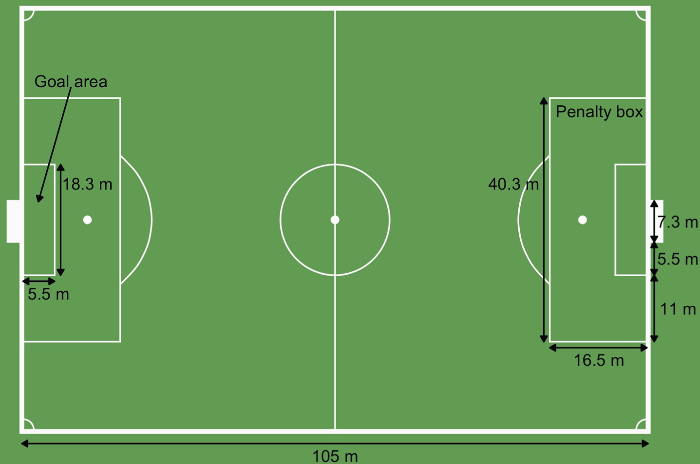
Finally, we also address errors with the coordinates of goal kicks. In the dataset, the starting coordinates for goal kicks are erroneously recorded at either (0, 70) for the home team or (105, 0) for the away team. Neither of these coordinates is possible –goal kicks should start within the attacking team’s goal area, a 5.5 by 18.3 meter box centered at the goal-line. Thus, we change the starting x coordinate of goal kicks to 0, and sample the starting y coordinates uniformly from the interval [25.85, 44.15], the y coordinates of the goal area.
3Pace-of-play metrics
3.1Framework
3.1.1Possession sequences
Ball possession is the amount of time a team possesses the ball during a game (Batorski, 2020). However, there is no widely accepted definition of what events conclude a possession and trigger a new one. We thus begin by creating a possession identifier that indicates the current unique possession in a game. In our definition, new possessions begin after a team establishes control of the ball. This occurs in the following situations: at the start of a half, when the team successfully intercepts or tackles the ball, after a shot is taken and after the opposing team last touches the ball before it goes out of bounds or commits a foul. A new possession can also begin even if the same team has possession of the ball. For example, if the ball goes out for a throw in for the attacking team, this indicates a new possession for the same attacking team. In addition, if the same team makes a pass after a sequence of duels (events in which opposing players contest the ball), this constitutes the same possession. Following the definition above, there are an average of 306 possessions per game in the merged data.
Along with the possession boundary rules defined above, we only consider a sequence of events to be a possession if it consisted of at least three or more pass or free kick events. Thus, situations where a team makes a single pass and loses control of the ball is not included in our analysis. Free kick shot and penalty kick events are excluded. Following these rules, there are an average of 5.5 events per possession.
3.1.2Metrics of pace
After creating a possession identifier, we first calculate the distance each event traveled. The east-west distances (δEW) are determined by the difference of the starting and ending x coordinates while the north-south distances (δNS) are determined by the difference of the starting and ending y coordinates. The total distances (δT) are the Euclidean distances between the starting and ending coordinates. Events are assigned an east-only distance (δE) if the pass travels toward the opposing goal. The major limitation with our distance calculations is that we assume the ball travels in a straight line from the start to end coordinates. In reality, passes rarely travel in a straight line and players will often dribble the ball before making a pass. However, the data does not provide information about the ball’s true trajectory and movement, so we are forced to make this assumption.
Next, we calculate the duration between events. For each event, the data only provides a timestamp in seconds since the beginning of the current half of the game. Thus, within each possession, the duration for an event is calculated as the difference of the timestamp of the following event and that of the current event. With this definition of duration, the last event in the possession sequence is not included in the calculation of pace.
We use the distance traveled and duration between successive passes and free kicks in the same possession to calculate four different measures of pace velocities: total (VT), east-west (VEW), north-south (VNS), and east-only (VE). VE differs from VEW in that only forward progress is measured, and any backward progress is excluded from the calculation (Yu et al., 2019). These four pace metrics are the average velocities of the event rather than the instantaneous velocities, since we did not have access to tracking data.
We define possessions as we do simply to help characterize when a team has the ball for an extended period of time. Since pace is intrinsically a measurement of a team’s style of play, we need to focus on periods in the game when each team is able to string a few consecutive passes together to obtain a stable and robust estimate of what the team’s pace is. This is why we require a minimum of three passes or kicks to determine a possession. This minimum requirement also accounts for the presence of outliers. There are certain passes that travel a far distance but in a short period of time, which we believe would constitute a data collection error. In addition, there are certain types of passes that are not reflective of a team’s pace. For example, if a defender clears the ball and the clearance is picked up by the opposing team, his team would technically have possession during the clearance, but this pass would not be representative of his team’s overall pace.
Given that the requirement of three passes or kicks per possession is an arbitrary choice, we conducted a sensitivity analysis on the minimum number of events per possession to ascertain that our overall conclusions are not sensitive to this threshold. We analyzed VT across the five leagues using possessions that contained at least two and at least five events. The calculated VT values are relatively similar across the three choices, and the overall conclusions are qualitatively similar.
3.1.3Spatial polygrid analysis
We divide the pitch into 294 equal, non-overlapping 5x5 meter square polygrids (Yu et al., 2019). VT, VEW, VNS, and VE for a given event are assigned to all polygrids that intersect with the event’s path. Polygrid i contains ni velocity values for the ni event paths that intersect it. For each of the 5x5 polygrids, we then take the median for each of the four different pace metrics defined in Section 3.1.2. Across the whole dataset, there are polygrids, particularly ones in the corners or along the attacking team’s goal line, that have very few recorded velocity values because only a few events intersect those polygrids. These polygrids often contain passes with extremely high velocities, most of which are due to tagging errors. Thus, the median is taken, instead of the mean, to account for the presence of outliers.
3.1.4Zonal analysis
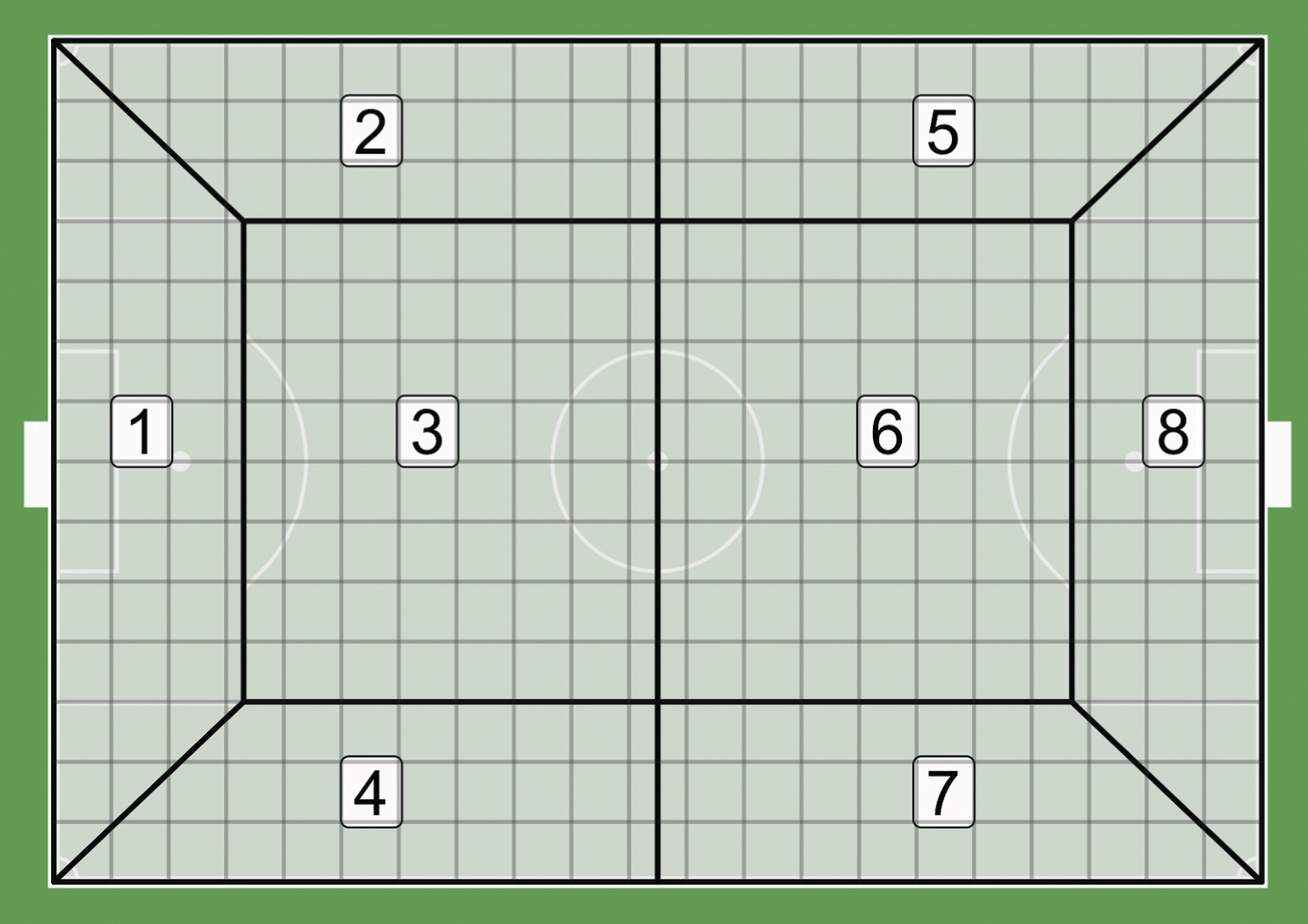
In this analysis, the pitch is divided the pitch into 8 zones. For each zone, we determined which of the 294 5x5 polygrids intersect the zone. As seen in Figure 2, there are some polygrids that fall into multiple zones. We then take the mean of the median VT, VEW, VNS, and VE values of those 5x5 polygrids to determine the aggregate velocities for the zone. This method is conducted in favor of another one that assigns an event’s velocities to all zones that intersect the path of the event. Our approach automatically factors in the event’s distance within the zone and is more resistant to outliers. For example, for a pass that intersects m different 5x5 polygrids in a zone, the zone’s aggregate velocity will be affected by that pass’ velocity m times instead of just once.
Fig. 2
Plot of the 294 polygrids and 8 zones overlaid on the pitch. The grey lines represent the polygrids and black borders represent the boundaries of the 8 zones. The team’s defending goal is on the left hand side.
3.2Results
3.2.1EPL pace (polygrid)
We first examine how pace in the English Premier League (EPL) differs among the 294 polygrids on the pitch. Figure 3 displays the velocities for all games played in the EPL. VT is the fastest in the polygrids within the opposing team’s penalty box and along the opposing team’s goal line. This is primarily due to higher VNS in those areas, which mainly comes from corner kicks. Corner kicks often have a higher velocity than most passes, and since most corners are taken into the 6-yard or penalty boxes, their trajectories will intersect with the polygrids along the goal line.
Fig. 3
Velocity by polygrid in the EPL for the 2017-18 regular season. Note that the scale of the four plots are different. The team’s defending goal is on the left hand side.
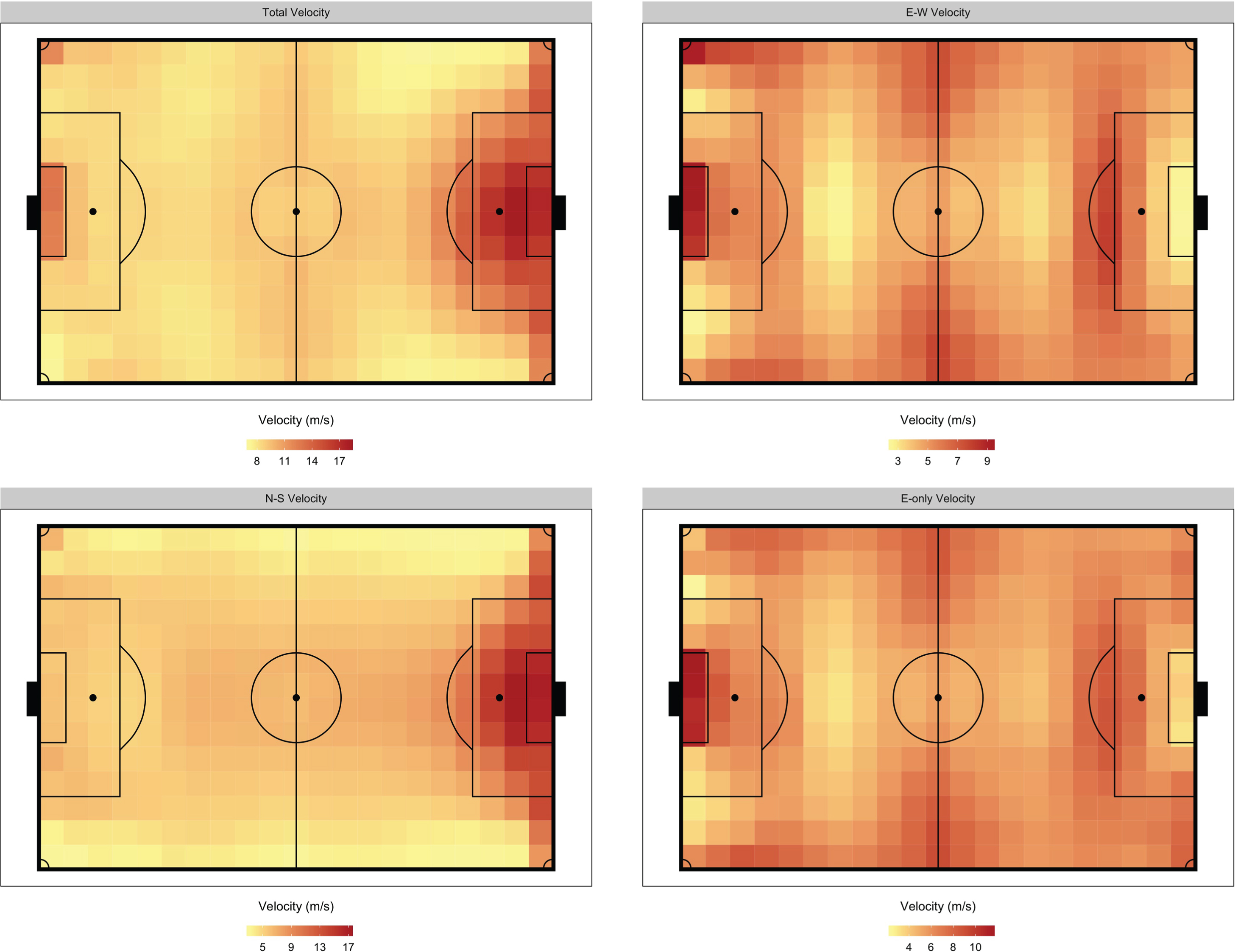
In the offensive half of the pitch, VT is slower along the left and right flanks and faster in the middle. This is primarily driven by the patterns in VEW and VNS. VEW is faster along the flanks and slower in the middle, while VNS displays the opposite pattern. However, since the scale of VNS is larger than that of VEW, VT is faster in the middle.
From the VE, it seems like the teams in the EPL prefer to advance the ball past the center line along the flanks, rather than down the middle. At the end of the 2017-18 season, 8 of the top 10 assisters were most often deployed as either left or right wingers or midfielders. This suggests that goal-scoring opportunities are more likely to come from the flanks, and thus pace is expected to be higher in those regions.
Another interesting result is that VE is relatively similar in the offensive and defensive thirds. Forward attacking pace (VE) is currently the most used metric of team-level pace (Harkins, 2016; Alexander, 2017; Silva, Davis and Swartz, 2018) but Yu et al. (2019) suggests that VE is not an ideal metric for measuring a team’s offensive capabilities because there are diminishing returns for advancing the ball forward. However, this decline in speed is only apparent in the polygrids around the 6-yard box. In most cases, players who receive the ball in this position would shoot, as these positions provide players with the most optimal shooting angles. However, VE does not decline in other polygrids in the offensive third. Central midfielders stationed around the outskirts of the penalty box could pass the ball to wingers on the left or right flanks. Even though the shooting angle worsens for the wingers, they can easily advance toward the goal line and cross the ball into the penalty box or cut back (Caley, 2019) to an onrushing player, both of which could lead to goal-scoring opportunities.
3.2.2EPL pace (zonal)
We then examine how pace in the EPL differs among the 8 zones. The results depicted in Figure 4 align with the observations from the Section 3.2.1. We confirm that VT is the highest in zone 8 and approximately 28-37% slower in the other seven regions. This is primarily due to the disparity among the VNS, particularly in zone 8. VEW is also roughly equal in all zones, which may have been hard to deduce from Figure 3. In addition, this confirms that VE is generally consistent across the pitch, which provides further evidence against the results found in Yu et al. (2019).
Fig. 4
Velocity by zone in the EPL for the 2017-18 regular season.
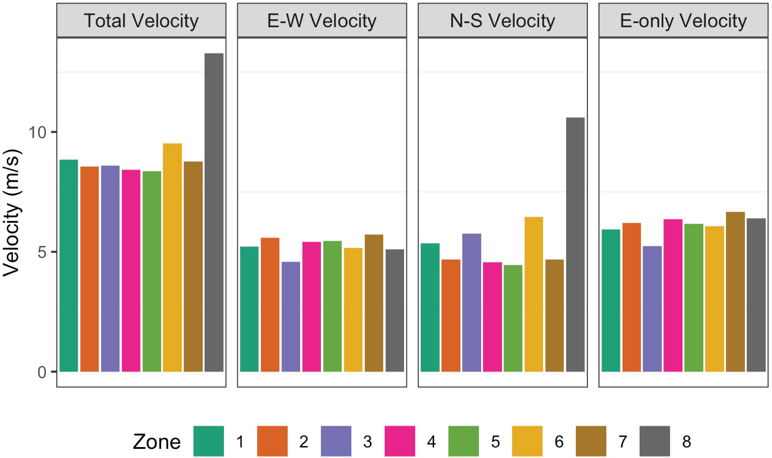
Symmetry between zones 2 and 4, and zones 5 and 7 may be expected. In the EPL, all four pace metrics for zones 2 and 4 are similar, but the velocities in zone 7 are slightly faster than those of zone 5. This suggests that teams in the EPL prefer to attack along the right flank since pace is slightly faster in that zone across all four pace metrics.
3.2.3Pace across leagues
Figure 5 shows the percent difference between the average velocities from the four other European leagues and that of the EPL. The results show that the Bundesliga plays faster than the EPL, while the other three leagues generally play slower than the EPL.
Fig. 5
Percent difference in velocity by zone relative to the EPL for the 2017-18 regular season.
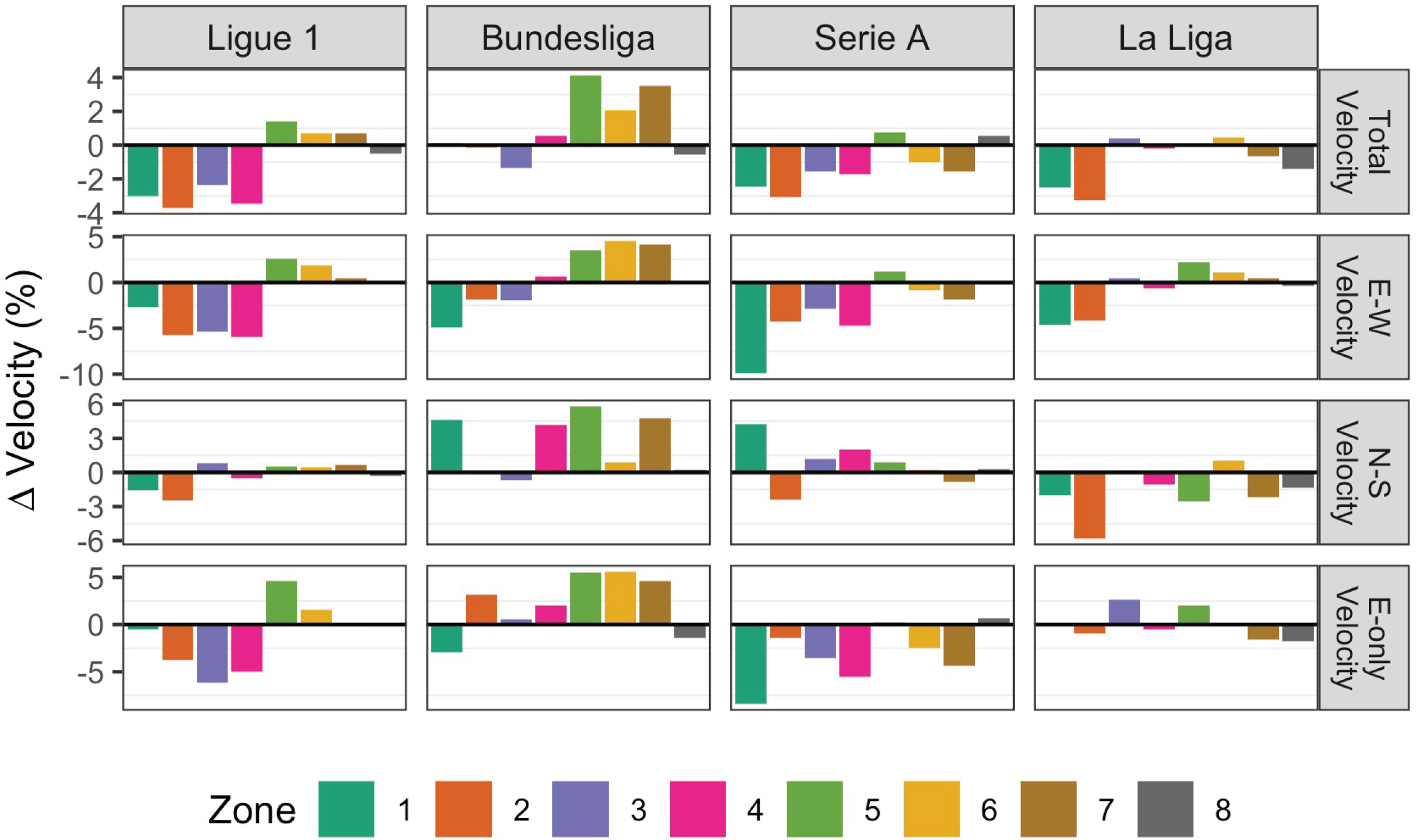
In Ligue 1, VT is approximately 1% faster in zones 5, 6, 7, and is primarily driven by changes in the VEW, as VNS is relatively similar to that of the EPL. This could be due to the fact that the average number of goals scored per game is slightly higher in Ligue 1 than in the EPL (2.72 vs. 2.68), as faster pace in the offensive half can yield more goal-scoring opportunities. In addition, the 2017-18 season saw the transfer of Neymar from Barcelona to PSG and the emergence of Kylian Mbappe. While Ligue 1 is often described as a poor attacking league, the advent of this formidable offensive duo may have reinvigorated the league’s attacking presence (Gibney, 2017).
Differences in the offensive half are most notable in the Bundesliga. VT in the Bundesliga is 2-4% faster in zones 5, 6, 7 and is driven by an increase in both the VEW and VNS. The increase in VT could have also been due to a higher average number of goals scored per game compared to the EPL (2.79 vs. 2.68). Additionally, Bundesliga players are more likely to create scoring chances and take more shots than those in the other four leagues (Yi et al., 2019), which is corroborated by the fact that the VE in zones 5, 6 and 7 are approximately 3-5% faster than the EPL.
Pace in Serie A is generally slower and primarily driven by a decline in VEW across seven zones, with the most noteworthy decrease occurring in zone 1. In terms of raw velocity values, this difference is approximately 1 meter per second. Unfortunately, nothing in the data or the available literature provides any further insight on this phenomenon. In addition, the average number of goals scored per game in Serie A is the same as in the EPL, which could have contributed to the similarities in pace in the offensive half between the two leagues.
La Liga displays the smallest difference in pace, with slightly slower velocities in zones 1 and 2. We initially expected La Liga teams to have the slowest velocities in the defensive half, as they are known for playing out from the back, a common tactic in which teams begin passing in their defensive third. This type of build-up play can help increase the quality of passes into teams’ midfielders and forwards. Goalkeepers such as Keylor Navas of Real Madrid and Marc-Andre Ter Stegen of Barcelona both possess excellent ball control and distribution skills, which thus allows their teams to start plays from the back. In recent years, more EPL teams have been adopting this tactic. Manchester City, with goalkeeper Ederson, is one of the best teams at playing from out from the back. When Pep Guardiola took over in 2016, he sought to implement a system that plays out from the back, which requires a goalkeeper who is comfortable with the ball at their feet (Tanner, 2018; Nalton, 2019; Robson, 2019). Although this style of play has a myriad of benefits, not all teams are capable of executing this tactic. Playing out from the back requires precise passes, as one wayward pass could fall into the feet of an opposing player. Some goalkeepers, such as Tottenham’s Hugo Lloris, arguably one of the world’s best goalkeepers in terms of anticipation and one-on-one situations, lack the ability to pick out the right passes and prevent their teams from adopting this tactic (Robson, 2019). The mixed success of playing out from the back in the EPL may have contributed to the slight difference in pace in the defensive half in comparison to La Liga.
In general, players from La Liga and the EPL also display the most similar performance-related match actions (Yi et al., 2019) and recorded a similar average number of goals per game (2.69 vs. 2.68), suggesting that only slight differences in pace should be expected between these two leagues.
3.2.4EPL team-level pace (polygrid)
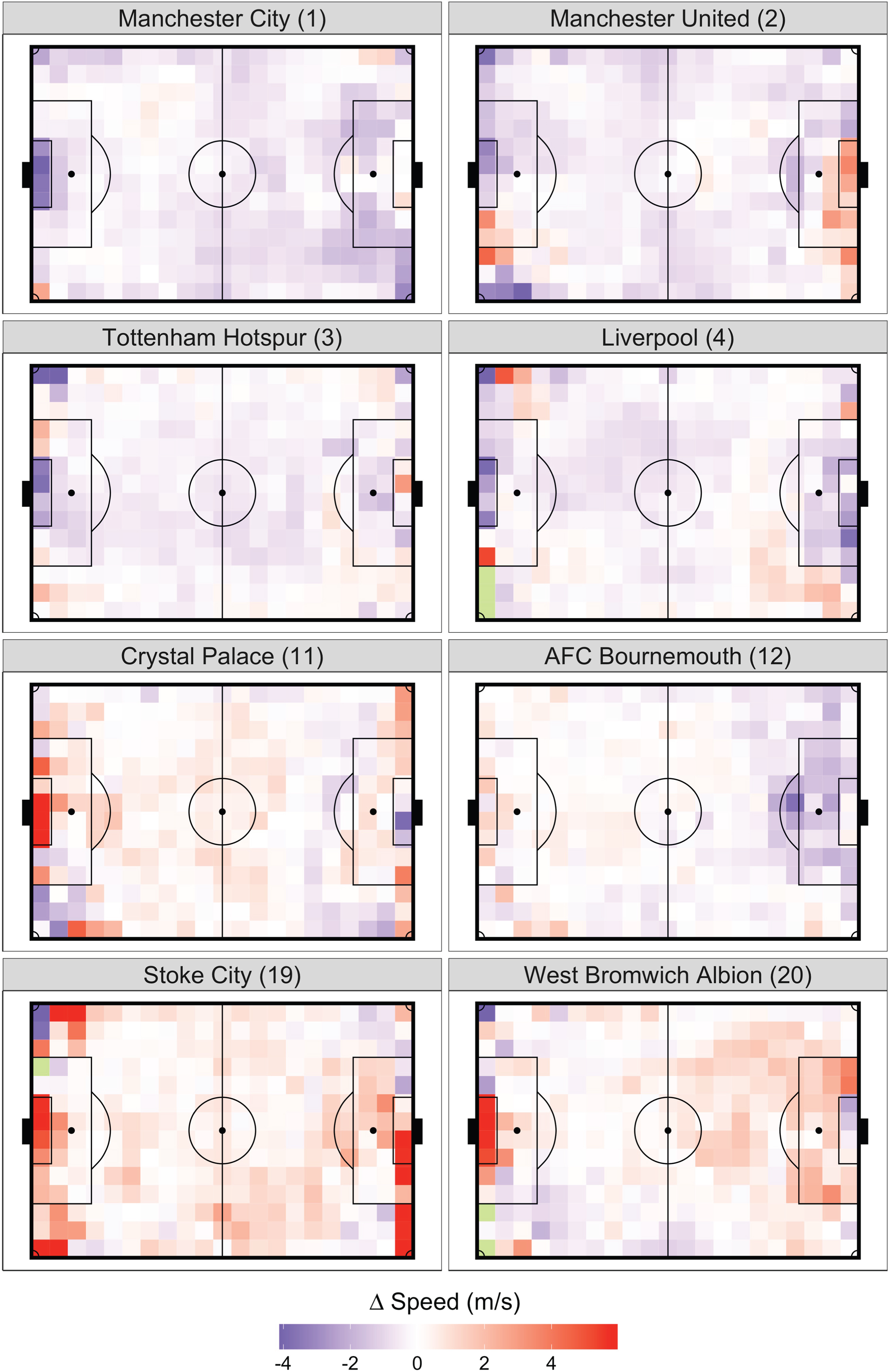
Figure 6 presents the difference between the VT in each 5x5m polygrid for 8 teams and that of the EPL average. None of these teams are faster or slower in all 294 polygrids, but the pace of the top six teams (Manchester City, Manchester United, Tottenham Hotspur, Liverpool, Chelsea and Arsenal) is generally slower than the league average. As we move down the league table, the polygrid velocities display more variation, but the four selected lower tier teams are faster than the league average in more regions on the pitch. It might seem odd that the top tier teams have a slower pace, but this is primarily due to the way we define pace. We expect these teams to maintain possession for a greater portion of the game. Thus, it follows that teams are more likely to maintain possession when making shorter, more controlled passes. In addition, goal kicks from the top four teams are relatively slower than the league average, with Manchester City’s having the slowest velocities. Although there is some variation, goal kicks from the bottom tier teams are generally faster than the league average. Since lower tier teams may not have possession for long periods of time, their goalkeepers may feel pressured to take longer goal kicks down the pitch, with the hope that one could create a goal-scoring opportunity. This is corroborated by the fact that Manchester City’s goalkeeper Ederson took 71% of his Premier League passes short, while every other goalkeeper, except for Liverpool’s Simon Mignolet, took less than 50% of their passes short (Spencer, 2017).
Fig. 6
Polygrid analysis of total velocity by team vs. EPL average while attacking. Select teams are ordered by final standings from the 2017-18 season. All units are in m/s. The team’s defending goal is on the left hand side.
4Modeling
4.1Variable and model selection
After creating the pace-of-play metrics, we want to evaluate their effectiveness when used as variables in models that predict the outcome of a game. We implement models with and without the pace metrics to determine if the model with the pace metrics achieve a higher accuracy. We only consider variables whose quantities are known before each game is played and did not include traditional post-game performance-based features, such as the number of shots or corners taken. Even though we incorporate a pace metric from the same game as a variable, we anticipate that they can be made into pre-game variables by substituting our pace metrics with historical measurements of pace.
Table 3 describes the predictors used in our baseline model. For each of the 1,826 games, the response variable, Full Time Result (FTR), describes the outcome with respect to the home team. An FTR of 1 indicates that the home team won, while -1 indicates the away team won. Unbeaten is the home team’s current unbeaten streak leading up to a game. The streak resets to 0 when a team loses at home. For the first home game of the season, a team’s unbeaten streak from the 2016-17 season is used. For example, Manchester City went unbeaten in their last 12 home games in the 2016-17 season, so their Unbeaten value for their first home game is 12. For the 14 newly promoted teams, their Unbeaten value for their first home game is 0. This is because they played in a lower division, so their home unbeaten streak is not comparable to that of a team that played in the first division. Derby is an indicator variable, where 1 indicates that a game is a derby game. A game is marked as a derby game if the two teams are located in the same city (Manchester City vs. Manchester United) or if there is a historical rivalry (El Clásico). League specifies which of the five leagues the game takes place in and Team provides the name of the home team.
Table 3
Description of modeling variables
| Variable | Description | Values |
| Response | ||
| Full Time Result (FTR) | Outcome of a game with respect to home team | 1 (Win), 0 (Draw), -1 (Loss) |
| Predictors | ||
| Unbeaten | Current home unbeaten streak (win/draw) | 0 to 19 |
| Derby | Indicates if game is a derby | 0 (No), 1 (Yes) |
| League | League that game takes place in | EPL, Ligue 1, Bundesliga, etc. |
| Team | Name of the home team | Liverpool, Barcelona, etc. |
Table 4 describes the pace variables. For each game, we conduct a zonal analysis of VT for the home and away teams. We take the median of the median velocities of the 5x5 polygrids to determine the aggregate velocities for each zone instead of the mean of the medians. Lower tier teams have a smaller number of recorded events per game and are more susceptible to outliers in both the polygrid and zonal analyses. Thus, using the median of the median velocities makes these zonal velocities more resistant to outliers. Then we calculate the difference (home - away) in VT for each of the 8 zones. Let i ∈ (1, 2, …, 98) represent the home team and j ∈ (1, 2, …, 38) ((1, 2, …, 34) for teams in the Bundesliga) be the jth game team i plays during the season. Then
Table 4
Description of pace variables
| Variable | Description | Values |
|
| Sum of the differences in total velocity for all zones (1-8) for home team i and away team j | -88.93 to 67.72 (m/s) |
|
| Sum of the differences in total velocity for all zones in offensive half (5-8) for home team i and away team j | -80.68 to 45.55 (m/s) |
|
| Sum of the differences in total velocity for zones 5,7,8 for home team i and away team j | -79.1 to 39.74 (m/s) |
To evaluate the models, we first split the data into train and test sets. The test data, which is 21.5% of the full data, includes 2 home and 2 away games for each of the 98 teams, for a total of 392 games. We perform 4-fold cross validation on the training data and lastly assess model performance by predicting on the testing data. We propose a hierarchical logistic regression model, where the baseline category is draws and losses. In the dataset, there are 828 games that ended in a win for the home team and 998 that ended in either a draw or a loss. This model is preferred over other classification algorithms since we are concerned with both predictive power and interpretability.
We first construct a baseline model that only uses the predictors mentioned in Table 3. We then add one of the pace variables from Table 4 to determine if the addition of a pace variable improves the model’s accuracy. Only one pace variable can be added to the model since they are all highly correlated. Interaction effects between the baseline predictors and quadratic terms for Unbeaten and the pace variables are also considered, but none of these modifications significantly improved the predictive power of any model. We utilize accuracy and area under the curve (AUC) as evaluation metrics for the hierarchical logistic regression. We define accuracy as the proportion of correctly predicted outcomes (both wins, and draws and losses). True positive rate (TPR) is the proportion of wins correctly predicted by the model, and false positive rate (FPR) is the number of draws and losses that the model predicts to be wins, divided by the total number of draws and losses. The receiver operating characteristics (ROC) curve then plots the TPR against FPR. The AUC establishes a tradeoff between the two, ensuring that we maximize the TPR while minimizing the FPR. The higher the AUC, the better the classification; a perfect classifier has an AUC of 1 while a model whose predictions are all incorrect has an AUC of 0.
4.2Hierarchical logistic model
The baseline hierarchical logistic model (without any pace variables) is as follows:
(1)
In the modified model, another covariate is added for pace considerations; the pace variable that produces the model with the highest accuracy is
Recall that the baseline of the response variable is draws and losses. FTRij is the full time result (win vs. draw/loss) of the game and πij is the probability that home team i wins the game. αi represents the random intercept term for team i. We do not include a random intercept for League, as most of the variability between leagues is already explained by the variability between teams.
Table 5 displays the results of the hierarchical logistic models. The baseline hierarchical logistic model reports an accuracy of 63.52% and AUC of 60.57 on the test data while the best performing pace model, the one with
Table 5
Hierarchical logistic model results with 4-fold cross validation
| Model | Mean Accuracy | Mean AUC | Accuracy | AUC |
| Baseline | 58.29% | 56.53 | 63.52% | 60.57 |
|
| 58.06% | 56.32 | 65.56% | 62.8 |
|
| 59.7% | 58.27 | 63.78% | 61.16 |
|
| 59.91% | 58.52 | 64.29% | 61.68 |
We expect the pace model with
Tables 6 and 7 displays the log odds and odds ratios for all the variables used in the baseline and pace models, respectively. All the coefficients, except for Unbeaten in the baseline model, are statistically significant. We note that the log odds for
Table 6
Coefficients obtained from baseline hierarchical logistic model
| Predictor | Log Odds Ratio | Odds Ratio | p-value |
| (Intercept) | -0.24 | 0.78 (0.67, 0.92) | <0.01 |
| Unbeaten | 0.03 | 1.03 (1, 1.07) | 0.06 |
| Derby | -0.9 | 0.41 (0.24, 0.69) | <0.01 |
Table 7
Coefficients obtained from pace hierarchical logistic model
| Predictor | Log Odds Ratio | Odds Ratio | p-value |
| (Intercept) | -0.29 | 0.75 (0.64, 0.88) | <0.001 |
| Unbeaten | 0.04 | 1.04 (1.01, 1.08) | 0.02 |
| Derby | -0.8 | 0.45 (0.27, 0.76) | <0.01 |
|
| -0.05 | 0.95 (0.94, 0.97) | <0.001 |
5Discussion
Our findings show that although pace varies considerably, it is generally highest in the offensive third of the pitch, relatively consistent across leagues, and increases with decreasing team quality, though there is much more variability in pace among the bottom tier teams. This observation is most noticeable in a team’s goal kicks. Top tier teams may feel more confident playing out from the back and may be less likely to take longer goal kicks. On the other hand, bottom tier teams may struggle to maintain possession for a long time, so their goalkeepers may feel pressured to take longer goal kicks, with the hopes that one could lead to a goal-scoring opportunity. We also see that teams vary in their ability to attack and defend pace in different regions on the pitch.
Forward attacking pace (VE) is currently the most used metric of team-level pace (Harkins, 2016; Alexander, 2017; Silva, Davis and Swartz, 2018), but Yu et al. (2019) notes that VE decreases drastically as teams move into offensive regions on the pitch and is thus not an ideal metric for measuring a team’s offensive capabilities. However, our findings show a contrasting result. VE only declines in the polygrids in front of the goal, but not in other polygrids in the offensive half. Since VE in the offensive half is also comparable to that in the defensive half, we believe that VE is an appropriate metric to gauge team-level pace.
Although we extracted meaningful findings from the pace metrics, there are limitations with the available data and methodology. The first is the presence of inaccurately tagged events. Incorrectly labeled coordinates or timestamps can affect the calculation of the pace metrics. In addition, we assumed that the ball always traveled in a straight line, as we did not know the true trajectory of the ball or if a player dribbled the ball before passing. Another limitation is the lack of player tracking data, as this type of data is not widely publicly available. Player tracking data could provide more information about the true, 3D trajectory of the ball, thus giving us more robust and accurate pace metrics. Lastly, many of the explanations we provided for our results are hypotheses that we cannot fully verify. We are unsure if some of our results are simply due to noise in the data or if they actually hold across seasons.
While the models perform adequately at predicting the outcome of a match, it is worth pointing out some limitations. We only had 1,826 regular seasons in our dataset, so creating train and test sets further reduced the amount of data used to train the models. Another limitation is the lack of uncorrelated pre-game variables. We tried other variables, such as the number of points a team accumulated last season and the number of top 100 players that play for a team. Unfortunately, they are all extremely correlated with one another and the Unbeaten variable. We also considered variables such as the average age of a team’s players and the market valuation of a team’s players, but are unable to find these values on a game-by-game basis. Due to this limitation, we note that our baseline model is a relatively simple model. However, the sole purpose of this model is to determine if the addition of a pace metric improves its prediction. Our findings show that pace is not useful in predicting the outcome of a match. This result, along with the counter-intuitive findings from Silva, Davis and Swartz (2018), emphasizes that the measurement and impact of pace is a nuanced subject that requires more research.
5.1Future steps
The scope of this analysis discusses pace on a team and league level. However, pace can also be evaluated at the player-level. Future work includes quantifying player-level pace and evaluating passing networks using network analysis to determine a player’s value within a team and if that player’s value has changed across the season. We can also examine the impact of pace on events in the game, such as pace before a shot is taken and how pace impacts a team’s pass completion rate.
Our models may perform better if we are able to incorporate other pre-game covariates. Variables related to the ranks of the home and away team and the competitiveness of a league could help improve the predictions of the baseline model. We could also incorporate data from across multiple seasons. This would not only provide more data to train the models on but could also help quantify heterogeneity across seasons, if included as a random effect in the hierarchical logistic model. Once better models have been developed, we would then investigate the usefulness of the pace metrics in these models.
References
1 | Alexander, D. , (2017) . Sequencing unmasking true creative forces. Premier League Football News, Fixtures, Scores & Results. Available at: https://www.premierleague.com/news/489392 [Accessed April 13, 2021]. |
2 | Batorski, E. , (2020) . Ball possession in football - how it’s calculated and how it matters: STATSCORE - News Center. STATSCORE. Available at: https://blog.statscore.com/ball-possession-in-football-how-its-calculated-and-how-it-matters/ [Accessed April 13, 2021]. |
3 | Caley, M. , (2019) . Two of soccer’s most dangerous passes. The Washington Post. Available at: https://www.washingtonpost.com/news/fancy-stats/wp/2014/10/16/two-of-soccers-most-dangerous-passes/ [Accessed April 13, 2021].= |
4 | Davies, J. , (2016) . Mourinho’s midfield pressing and 6-3-1 halts Klopp’s side. Spielverlagerung. Available at: https://spielverlagerung.com/2016/10/19/mourinhos-midfield-pressing-and-6-3-1-halts-klopps-side/ [Accessed April 13, 2021]. |
5 | Ferrero, V. , (2013) . The Effectiveness of Using Pace, eFG%, 750 TOV%, ORB%, FT/FGA, and ORtg to Predict the Outcome of NBA Regular Season Games. |
6 | Gibney, A. , (2017) . Ranking Ligue 1 Sides on Their Defensive Strength. Bleacher Report. Available at: https://bleacherreport.com/articles/2321750-ranking-the-ligue-1-sides-ontheir-defensive-strength [Accessed April 13, 2021]. |
7 | Harkins, J. , (2016) . Introducing a Possessions Framework. Stats Per-form. Available at: https://www.statsperform.com/resource/introducing-a-possessions-framework/ [Accessed April 13, 2021]. |
8 | Harkins, J. , (2016) . Introducing a Possessions Framework. Stats Per-form. Available at: https://www.statsperform.com/resource/introducing-a-possessions-framework/ [Accessed April 13, 2021]. |
9 | Knutson, T. , (2013) . A look at pace in football. Available at: https://bitterandblue.sbnation.com/2013/1/24/3908816/football-soccer-analytics-pace [Accessed April 13, 2021]. |
10 | Knutson, T. , (2015) . Pace and Margin for Error. StatsBomb. Available at: https://statsbomb.com/2013/11/pace-and-margin-forerror/ [Accessed April 13, 2021]. |
11 | Lawrence, T. , (2015) . Europe’s Most Direct Teams. Deep xG. Available at: https://deepxg.com/2015/11/06/europes-mostdirect-teams/ [Accessed April 13, 2021]. |
12 | Minkus, K. , (2017) . Examining Pace in MLS. American Soccer Analysis. Available at: http://www.americansocceranalysis.com/home/2017/3/9/examining-pace-in-mls [Accessed April 13, 2021]. |
13 | Nalton, J. , (2019) . Play Up Or Play Out: The Myths And Legends Of Playing Out From The Back.World Football Index. Available at: https://worldfootballindex.com/2019/09/playing-outfrom-the-back-tactics-analysis-guardiola-lillo/ [Accessed April 13, 2021]. |
14 | Pappalardo, L. , et al., (2019) . A public data set of spatio-temporal match events in soccer competitions. Nature News. Available at: https://www.nature.com/articles/s41597-019-0247-7 [Accessed April 13, 2021]. |
15 | Patzig, P. , (2021) . Soccer tactic: Why is the 4-1-4-1 the best formation. Available at: https://www.coachbetter.com/new-posts/soccer-tactic-why-is-the-4-1-4-1-the-best-formation/ [Accessed April 13, 2021]. |
16 | Robson, S. , (2019) . Why playing out from the back has brought mixed results for Premier League clubs. ESPN. Available at: https://www.espn.com/soccer/english-premier-league/story/3945761/why-playing-out-from-the-back-has-brought-mixed-results-for-premier-league-clubs [Accessed April 13, 2021]. |
17 | Silva, R.M. , Davis, J. & Swartz, T.B. , (2018) . The evaluation of pace of play in hockey. Journal of Sports Analytics 4: (2), pp. 145–151. |
18 | Spencer, J. , (2017) . Stats Reveal Just How Suited New #1 Eder-son Is to Pep Guardiola’s Man City System. 90min.com. Available at: https://www.90min.com/posts/5833855-stats-reveal-just-how-suited-new-1-ederson-is-to-pep-guardiola-s-man-city-system [Accessed April 13, 2021]. |
19 | Tanner, R. , (2018) . Guardiola reveals the ‘hardest decision’ of his career. Mirror. Available at: https://www.mirror.co.uk/sport/football/news/pep-guardiola-explains-axing-joe-13445300 [Accessed April 13, 2021]. |
20 | Wright, N. , (2018) . Jose Mourinho under pressure to attack when Manchester United host Liverpool. Sky Sports. Available at: https://www.skysports.com/football/news/11667/11278517/jose-mourinho-under-pressure-to-attack-when-manchester-united-host-liverpool [Accessed April 13, 2021]. |
21 | Yi, Q. , et al., (2019) . Differences in Technical Performance of Players From ‘The Big Five’ European Football Leagues in the UEFA Champions League. Frontiers. Available at: https://www.frontiersin.org/articles/10.3389/fpsyg.2019.02738 [Accessed April 13, 2021]. |
22 | Yu, D. , et al., (2019) . Playing Fast Not Loose: Evaluating team-level pace of play in ice hockey using spatio-temporal possession data. Proceedings of the 2019 MIT Sloan Sports Analytics Conference. Available at: https://arxiv.org/pdf/1902.02020.pdf [Accessed April 13, 2021]. |


