
A comprehensive approach to predict auction prices and economic value creation of cricketers in the Indian Premier League (IPL)
Abstract
The Indian Premier League (IPL), the most successful cricket tournament in India, has immensely grown in popularity. Unlike similar tournaments like Major League Baseball and the UEFA Champions League, their models cannot be replicated due to the dynamic pricing nature of player auctions. The research intends to generate a predictive model that predicts the auction price of a player using key quantitative variables. The players were categorised by batsmen, bowlers, and all-rounders. Due to the holistic hedonic nature of the model, equations were formed to predict a player’s future performance, in terms of measurable points, and to extrapolate economic value creation given a budget constraint. This study provides insights on the player’s economic value by comparing the auction price paid vs. the player’s actual performance. This new approach to modelling in cricket games not only aims to produce more accurate results using the hedonic pricing method, but also enlightens an introduction to a more holistic modelling process to intricately understand the profiting avenues for team owners to reverse-engineer value additions of players at each level and position. Finally, this model, which considers the factors an IPL franchise would, is being designed to be utilised in future IPL auctions.
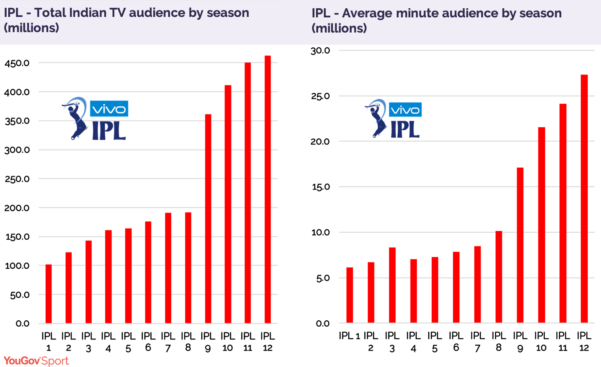
Fig. 1
Diagram representing the viewership of IPL across seasons (Can IPL’s Season 13 match Season 12’s Record popularity, 2020).
1Introduction
After 60 breath-taking matches over the course of three thrilling months across eight franchises (Chakraborty, 2021), the Indian Premier League (IPL) has rapidly become the most-attended cricket league in the world. A franchise-based T20 cricketing format tournament initiated in April 2008 by the Board of Control for Cricket in India (BCCI) (Mitra, 2010), IPL has attracted fans not only from India but also from across the world. Since its inception in 2008 where it attracted 100 million Indian viewers, its viewership has more than quadrupled to exceed 450 million in 2020 as shown in Fig. 1. A key factor of why rising numbers of fans tune in to watch these matches, as with any sport, is the players and their spectacular performances in matches as members of respective teams.
A bat-and-ball game that exists in different formats across the world, such as the T20 1 ODI2 and Test3, cricket is played and thoroughly enjoyed. It’s all about team spirit in this sport; it is a game that can only be won if all individuals put in effort by performing their respective roles. For example, a batsman focuses on making runs by running between the wickets as well as hitting the ball for boundaries, while a bowler aims to limit the runs scored by the batsman and take wickets (Importance of Cricket (game), 2016).
Fans eagerly await every season, every match, and are constantly glued to their screens to watch the finest and best performing players from many different countries. Each team plays against another twice, and the winner gets two points on the scoreboard per game. It continues to get thrilling as teams fiercely compete to get in the top 4 to be able to qualify for the playoffs4 . and then finally for the champion’s trophy. Another aspect that stands out is the fact that these are one of the most elite teams amongst many domestic teams internationally as portrayed by their spectacular participation in the Champions League Twenty 20 (2009 –2014), a competition that was played between the top domestic teams from different countries, in fact, 4 out of the 6 seasons were won by IPL teams (Champions League Twenty20 Cricket Team Records & Stats | ESPNcricinfo.Com, n.d.).
According to the BCCI, each franchise is mandated to have 16 players with at least 8 local players and 2 players from India’s under-22 pool of players. It can purchase up to 10 international players, although only 4 are allowed to play any game at once (IPL, 2020).
Given the massive pool of players available for teams to bid and potentially acquire, choosing a player who can contribute to the success of the team is a vital part of the process. With IPL, the acquisition of players is done through an auction-based model (see Appendix A), commonly known as the bidding game, in which franchises engage in bidding against one another to buy a specific player through the open market. Each team has the same amount to spend on the acquisition of players, with the requirement that teams spend a minimum of 75% of their purse size (IPL, 2020). Structured like an open ascending-bid auction, players are called in groups of players each based on their skill (see Appendix A). Ultimately, each player has an annual base salary that is determined by the players themselves prior to the auction, and each incremental bid starts from its base with a fixed amount, depending on the different brackets of bids (IPL, 2020).
The bidding process is inherently dynamic in nature, as franchises have to frequently realign their strategy after each bid by taking into consideration multiple factors. Most importantly, they have to take into account a player’s potential contribution to the team as well as predicted economic value creation of the player, which should be formulated quantitatively and in an objective manner (Singh et al., 2010). However, they also consider what other franchises are bidding to understand the dynamics of demand for each player and accordingly use game theory strategies to acquire players (Singh et al., 2010).
Historically, team selection and auction bidding has been subjective involving a combination of qualitative judgements, notions, heuristics, or other crude methodologies (Ahmed et al., 2013). This has resulted in significant discrepancies between the amount paid for the players and their actual performance, as in the case of players like Yuvraj Singh, who was sold at 16 Crore Rupees (in the IPL 2015 Auction), the highest ever, while his performance was way off the mark. This had sparked a lot of debates about the valuation of players that caught the media’s attention. There were a couple of more such deviations like Shane Watson in 2016, sold for 9 crore and 50 lakh rupees, even though he did not display good performance. Another one that ignited discussions about economic value versus performance was Jaydev Unadkat in 2019, auction price of Rs 8 Crore and 40 lakh, while the performance was much below the average.
After analysing the above examples, it seems fair to conclude that the difference between payment and performance could be improved and minimized by approaching the valuation of players quantitatively and objectively through predictive Machine Learning models. This viewpoint is further supported through several studies on players’ compensation. First, a research paper by Deep et al. involves the usage of a machine learning based model to predict the performance of the batsmen and bowlers (Deep et al., 2016), therefore, effectively reasoning the use of a more data-driven method to predict player’s performance. Moreover, taking a similar empirical and quantitative approach, in another research study, the authors prove the theory that the auction prices should have a correlation and be a reflection of the quantitative performances of the players (Depken et al., 2010), which, in fact, is the underlying idea in this research study.
Moreover, Karnik, A. (2010) showed the inefficiency in valuing the auction prices of the players by the franchises, which also acts as the embedded assumption and the reason why an equation has been constructed to objectively predict the auction price for a player.
This study thus sought to develop a methodology that could be applied to future auctions by teams for the valuation of players to optimise budget allocation, in other terms, to bridge the gap between auction price and the economic value created.
2Motivation
As highlighted earlier, it is clear that there is a gap between the monetary value (salary paid to the player) and the player’s value add in terms of performance points, which leads to the conclusion that teams are making suboptimal and irrational allocations. Previous research in this domain has narrowly focused on players’ performance in the previous year, or has taken variables such as popularity which has exhibited negligible correlation to player performance, to decide players’ salary. Moreover, previous research efforts have not factored in the value addition of different positions in a team and how each player fits in the whole team.
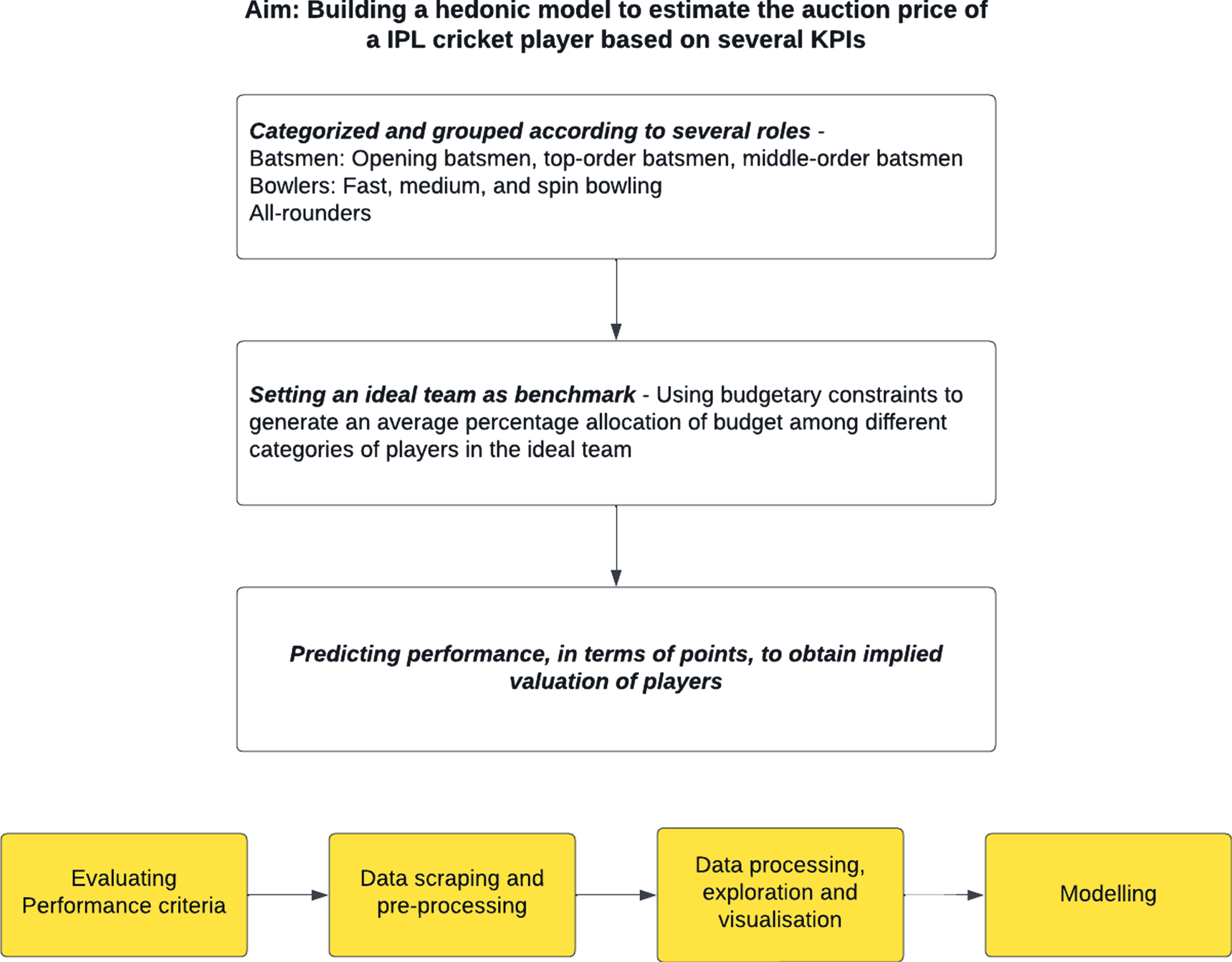
Fig.2
Pictorial representation of proposed methodology.
To address this problem, a holistic modelling process is needed and an intricate understanding of the nature of ways in which players can create opportunities for monetary value addition for the team owners. The modelling process takes into account not only the inherent dynamics of the bidding process, but also takes a broad approach to evaluating the historical performance across a wide variety of metrics of each player and across positions to reasonably predict player performance in an IPL season and determine their value addition, while factoring in anomalies and various psychological factors such as the Law of Averages5. It also factors in the improvement of the player over time and other non-performance attributes such as age. In agreement with research in this domain, the research appreciates the relevance of hedonic price equations in the modelling process and the convoluted, multicollinear nature of the variables involved in sports.
While this has theoretical implications to the sports analytics community at large, it also has several practical implications for teams in the Indian Premier League, and other tournaments with similar auction structures and team construction dynamics. Assuming historical statistics on the player, due to the inherent holistic nature of the model, model works reasonably to predict the future player performance and extrapolate that to player salaries relative to a team budget. It also takes into account only quantitative factors –which are easy to implement and extrapolate. However, inevitable so, it is difficult to implement for a new player, as we need to rely on preliminary cricket tournaments such as Ranji Trophy while accounting the relative performance against other players in the same tournament and use standardized means. However, due to the difference in quality of players between the players in the preliminary tournaments, it is difficult to compare standardized means across tournaments. The modelling process is designed such that if teams follow, they are likely to make significantly more optimal decisions and yield greater payoffs. However, if teams follow the same objective expectation of an ideal team, they are likely to run into a Nash Equilibrium, which may yield lower payoffs compared to if they were the only ones to employ the dominant strategy. They will run into a stalemate, given their budget constraint, and this poses as one of the limitations of this model.
3Proposed methodology
Through this research study, we aimed to investigate how player valuations could be determined in a systematic, data-driven manner with an accurate and reliable predictive Machine Learning (ML) model. More specifically, the model would estimate the auction price of a player based on several statistics. The inherent assumption of this model is that data from past performances can be harnessed and transformed into a powerful and predictive tool to estimate future player performances in the form of economic value creation of player.
Supervised learning methods were used throughout the process because the output of the hypothesis is available in the present data. In particular, linear regression was used for primary output of equations because of several reasons. Firstly, since the basis of research was hedonic pricing in principle, linear regression is the only model that permits constructing equations that are, in some form, a linear combination of the variables. Secondly, the algorithm assumes the data and the error residuals are normally distributed, which has been taken care of by standardization of data. Thirdly, by the embedded methodology, the algorithm accepts training data to be homoscedastic. Lastly, it assumes that variables are not collinear, and the methodology makes a sincere attempt to avoid collinearity, given the nature of the dataset. Most other supervised learning methods either use non-linear models that cannot be prescribed in equations, hence defeating the aim of making the model easily replicable. Within the context of a cricket game, whereby two teams of 11 players take turns to bat or field, players predominantly contribute to the team through their batting/bowling skills, therefore, their batting and bowling capabilities would play an important factor in the predictive ML model. An additional element would be to take into account a player’s contribution to the team performance.
4Creating an ideal team as benchmark
To develop a systematic model, the first step was to come up with an ideal team — how many players of each role needed for the squad (see Table 1). Furthermore, budgetary constraints were considered: the overall budget of the franchises was divided proportionally for each role, factoring in the reality that batsmen tended to be priced higher than bowlers, with all-rounders garnering the greatest proportion of the budget. After back testing these benchmarks against team constructions in the past across auctions, there were no teams that came close to the ideal team formation, and it is also apparent that team focused on popularity of players. Thus, to prevent error across the entire modelling process, skewing the results on surpluses and deficits, an ideal team benchmark was created.
Table 1
Ideal team composition and budget allocations
| Ideal Team | ||
| Player roles | No. of Players | Allocation |
| of Budget | ||
| Opening Batsman6 | 2 | 12% |
| Top-order Batsman7 | 2 | 12% |
| Middle-order Batsman8 | 2 | 10% |
| Fast bowler9 | 4 | 12% |
| Medium bowler10 | 3 | 8% |
| Spin bowler11 | 3 | 10% |
| All-Rounder12 | 7 | 26% |
The ideal team was derived from real-life data by reviewing the squads of all the Runner-ups and Champions of the past four IPL Seasons (2016–2019). These years were chosen due to the lack of precise data on squads prior to the 2016 IPL Season.
Next, the squads were categorized and grouped according to several roles (note that due to no international players-specific budget constraint in the IPL auction mandate, there was no need to include a specific allocation for international players as such). For example, the batsmen were divided into opening batsmen, top-order batsmen, and middle-order batsmen, respective to their different positions in the batting order, therefore, their opportunity to score and influence the outcome of the match differs as the number of balls faced is likely to vary, and, moreover, the ball gets older resulting in it tending to spin more –a disadvantage for any batsman. The opening batsmen have to not only face the new ball, but are also intended to serve the team off to a good start, and are thus intended to have patience, a sound technique and be good defensively. In limited-over games like IPL, the top-order batsmen and middle-order batsmen serve the purpose of not only maintaining the momentum of the score but also serve as pinch-hitters (score quick runs without fearing a wicket) to maximize their team runs. Therefore, the opening batsmen are likely to be most skilled, hence, will be paid the most usually. In addition, the bowlers have been divided into fast, medium and spin according to the style and the pace of bowling, while they may also have different objectives in terms of taking wickets and limiting the number of runs conceded. While fast bowlers rely on speed to make batsmen misjudge the speed/bounce and faulter, medium and spin bowlers rely on a variety of flight and spin to deceive batsmen. On the other hand, all-rounders tend to be good with both batting and bowling, and have varying levels of skill in each domain. Usually, all-rounders have their own expertise, signified by the prefix to their position, such as “Spin all-rounder” signifying they are better on average at spin bowling than batting. Hence, with different roles these players are likely to be valued differently, therefore, creating emphasis on the need for the categorization of players.
By taking the average of the number of players in each of the categories from all the squads and rounding it to the nearest integer, an ideal team composition was determined. Alongside, the past budget allocations of the respective squads — i.e. proportions allocated to each role, were then computed to generate an average percentage allocation of the budget to be allocated amongst the different categories of players in the ideal team.
At the same time, it is important to point out that this allocation of the budget assumes that the T20 format of cricket is a batsman’s game. The T20 format is essentially a limited overs game, whereby the aim for the players of the batting team is to put up a high score on the board, while the bowling side mainly strives to limit the total number of runs scored, rather than taking wickets. Furthermore, the Powerplay fielding restrictions — only two fielders are permitted outside the 30 yard circle surrounding the wickets — pose a drawback for bowlers, while encouraging batsmen to hit freely without much risk. To provide further evidence to this viewpoint, in one such study by Singh et al. (2010), an interesting and logical aspect in the paper is that between batting and bowling, more weight is given to batting as compared to bowling. This is because every player can contribute to the team as a batsman, but not everyone is required to contribute as the bowler.
Therefore, a higher proportion of the budget was allocated to the batsman.
The data above (see Table 1) would aid in the subsequent stages of the methodology, especially towards the end, when the predicted performance, in terms of points, needs to be scaled to the valuation of players, in monetary terms — Indian Rupees (🙼), as it is important to answer these questions:
1 How many players of each role should a franchise purchase?
2 For these many players, how much of the budget should the franchise allocate to that specific role?
5Stages of investigation
The research study was conducted in four stages with the following aims:
Step 1: Evaluating Performance Criteria: This step was conducted to identify the set of features that best predict future performance of a player in the IPL.
2 Step 2: Data scraping and pre-processing: Next, the data were collected and organised into an analysable format by using Microsoft Excel and Python.
3 Step 3: Data Processing: Computations were performed to improve the consistency and analysability of the data.
4 Step 4: Data exploration and visualisation: Python tools were used to create visual representations to investigate and represent the correlation between the independent factors and the dependent variable of the ML model.
5 Step 5: Modelling: Various ML models were attempted to design the desired ML Model that could predict an estimate of the auction price for a player in the IPL with accuracy.
6Evaluating performance criteria
In order to achieve an objective evaluation of a player’s utility to a team, focus was placed solely on individual performance statistics rather than team performance. Moreover, to ensure objectivity of the model, qualitative and subjective attributes like team training, technology used, coach quality and team chemistry were ignored.
Based on the aforementioned considerations, the data of each player were evaluated based on the following “abilities” described below. It is important to point out that each of these abilities was evaluated independently for the different roles and even sub-categories within these roles (such as Opener/Middle-order /Top-order batsman for batting; Fast / Medium / Spin for bowling; and Wicket-keepers13 to ensure that the objective of a diversified skill set in a composite team is optimised.
Batting Ability. Raw data –Number of Innings14 , Not Outs15 , Total runs scored, Highest Score16 , Total Number of 4 s, Total Number of 6 s, Number of 50s17 and Number of 100s18 — were collected for each batsman. The following composite parameters, “Batting Average” and “Batting Strike Rate” were used to evaluate a player’s batting ability in order to ensure that the statistics were normalised and experience bias19 was eliminated:
Bowling Ability. Raw data –Number of bowling innings, Number of overs, Number of runs conceded, Number of wickets taken, Number of 4 Wicket hauls, Number of 5 Wicket hauls — were collected for each bowler. The following composite parameters were used to evaluate a player’s bowling ability:
Fielding Ability. Raw data were collected for each player, based on the total number of catches made by the player throughout the season. However, the fielding skills were discounted, while analysing the performance statistics of players due to the subjective and biased nature of the data. The number of catches taken by a player highly depends on the position of the fielder, for example, slips20 could simply have more opportunities to catch as compared to other fielding positions. Moreover, the fielding ability also does not take into account the number of dropped catches due to lack of sufficient data, which has a vital role in determining a fielder’s skillset. Therefore, it seems as the best possible choice to not consider it, to avoid any subjectivity in the prediction of the valuation of players.
Other Factors. Other factors included the Age, Role, and International/Domestic were also used, due to their relevance to the evaluation of the player performance and team composition limitations as per the guidelines by BCCI.
Age: Player age was introduced as a quantitative indicator of player agility. Age is an interesting factor for consideration: while old players may be less agile, they possess more experience and can contribute to the team through their leadership potential and team chemistry building skills, as compared to younger players (Herridge et al., 2017).
Role: Wicketkeepers, all-rounders, fast bowlers, spin bowlers, medium pace bowlers, opening batsman, top-order batsman and middle-order batsman are used as categories to gauge any differences in player valuations respective to the roles as they demand different skill sets from players.
International/Domestic: It can be helpful to understand if there is any inherent skew in valuations between domestic players and international players, given the IPL auction design of limiting international players in a team.
Since roles and international/domestic were categorical, one-hot-encoding was done to convert categorical variables to discrete numerical data and remove any potential biases that could result from other types of encoding methods.
The batting and bowling abilities were also evaluated across cricket game situations and formats to ensure that the different skill sets of each player are captured in the dataset. For example, some of the bowlers may be specialised to bowl only in the death overs or even in only the powerplay overs, therefore, it is important to capture such specific skills of a bowler. In addition, the T20 International Format also is an important indicator of recent performance as these games take place all year round, therefore, being a good predictor for performance of the player in the IPL. The following are the different game situations and formats considered:
Death format: Death overs in IPL often refer to the last 5 overs of a limited overs match, in which the batting side often bats aggressively to maximise its runs, while the best bowlers in the opposing team would attempt to minimise the number of runs. Measures a batsman’s ability to score as many runs, without prioritizing on his wicket and bowler’s ability to not only limit runs, but also take wickets.
• Powerplay format: Powerplay overs are usually the first six overs of each innings, in which fielding restrictions apply. Reflects a batsman’s ability to retain his wicket and a bowler’s ability to take as many wickets as possible. As there are fewer fielders protecting the boundary line, it tends to favour the batting side, thus incentivising batsmen to score runs.
• T20 International format (T20I) (Two International teams, 20 overs each): Batting and bowling statistics in this format are also considered to recognise the player’s performance in another similar format which has same playing rules but gives a different dimension as these matches are held under different ground conditions.
The batting and bowling variables in these particular game situations and formats, that are mentioned above, are considered such as Batting Average in Powerplay Overs, Batting Average in Death overs and Batting Average in T20I –these examples are of three different variables taken into consideration that outline the Batting average of the player, but in different situations and formats –amongst others.
Table 2
Summary statistics of different types of Batsman across formats
| Opening Batsman | Top Order Batsman | Middle Order Batsman | ||
| Match | Batting Average | 32.9 | 39.3 | 28.4 |
| Batting Strike Rate | 127.8 | 127.8 | 124.0 | |
| Powerplay Overs | Batting Avg Powerplay | 38.9 | 52.8 | 32.0 |
| Batting SR Powerplay | 121.4 | 109.6 | 134.7 | |
| Death Overs | Batting Avg Death | 56.5 | 40.4 | 24.5 |
| Batting SR Death | 180.4 | 166.2 | 147.8 |
A multiple hypothesis test was conducted containing each of the batting and bowling variables for each of the two pairs comparing the match average with powerplay overs and death overs (null that it yields the same average statistics as the match average). It was found that at the 0.05 significance level, none of the variables could be discarded (failed to reject the null) at each of the situations –powerplay and death overs. This indicates that there exists statistically significant difference in KPIs across situations and formats of overs, yielding the conclusion that three datasets need to be used for training to obtain a broader picture of performance of each player, whether batsmen or bowlers.
As is evident, and proven by the multiple null hypothesis test, there exist statistically significant difference in KPIs for each of the over formats vs the match average.
For Batting, it is evident that on average, the strike rate for batsmen in powerplay overs is lower than the match average, keeping in line with the argument that batsmen tend to go slow, play cautiously and slowly build momentum when the conditions do not favour them. On the other hand, in death overs, consistent with the argument, batsmen have a much higher Strike rate as they tend to become pinch-hitters, trying to maximize runs at the risk of their wicket.
For bowlers, it is evident that for death overs, the economy rate is the highest while the average and strike rate is the lowest as compared to the other groups. This is consistent with the argument that in death overs, batsmen aim to hit the maximum runs and play risky shots in cognizance of the risk of getting out. On the other hand, for powerplay overs, on average, the economy rate is the lowest while the strike rate is the highest even though the average is below match average. This is consistent with the argument that in powerplay overs, batsmen tend to conserve their wicket and play safe to build momentum, and hence do not play risky strikes which would yield in 4 s or 6 s.
Uncontrollable Variables. In the game of cricket, various uncontrollable factors, such as game venue, weather, coin-toss result, and field condition, could undoubtedly impact the performance of a player. However, due to its inability to be quantified and the difficulty in obtaining aggregate statistics of a player, these attributes were not included.
7Data scraping and pre-processing
In this step of the methodology, the data is collected, which was aggregated, cleaned, corrected, and missing values were filled/dropped to ensure coherence, consistency, and completeness. This preparation is vital to ensure that the process of predictive modelling –that will be performed in the subsequent stages –would be efficient.
The dataset consists of 43 batting, bowling, and fielding attributes across IPL and T20 International games, powerplay and death overs, from 2013–2019. Data gathered were limited to the years after 2013 because of the following reasons. There was lack of transparency of data for auctions before 2012: salaries were not disclosed, lack of adequate performance data, etc. The year 2020 was also not taken into consideration due to a lack of data. Moreover, due to the pandemic, the sample size of matches for most of 2020 was below the statistically significant level for the data to be considered.
To scrape data for players, Python libraries were used to extract data from freely available websites,21 . web datasets, research papers as well as games’ scorecards and commentaries. The most frequently used sources for extracting raw data include: http://www.iplt20.com, http://www.espncricinfo.com, http://www.icc-cricket.com, http://www.data.world, http://www.kaggle.com, http://www.cricsheet.com, http://www.cricbuzz.com. Often, rather than aggregate data for players, ball-by-ball data were available for IPL and T20I games, and some features such as Powerplay and Death overs performances were not publicly available. Thus, appropriate classes and functions were programmed in Python to convert ball-by-ball data to aggregate performance statistics. Furthermore, as the 2018 data for T20I games were not publicly available, our model could not be tested for the subsequent years of 2019 and 2020. Nonetheless, we were able to back test our model with several years to make sure our model can still predict a good estimate of the IPL auction price of a player.
8Data processing
The objective of this phase is to develop a model in which the IPL Performance statistics over a two-year period have a strong correlation to performance in the succeeding year (as reflected by IPL Fantasy Points scraped from the official IPL website). Using the predictions of the IPL Fantasy points –a set of points formulated by IPL that indicates true performance of a player –in the succeeding year, an economic value can be assigned to how much a team should be willing to pay to that player. The dataset was thus refined to create separate data sheets designed to relate player performance statistics over a two-year period and the IPL Fantasy points calculated at the end of the succeeding season. For example, 2018 IPL Season Fantasy points were taken as the dependent variable, while performance statistics containing players with data over 2016 and 2017 were considered. A two-year period was selected to ensure adequate data points to mitigate the effects of psychological law of averages22 and any other anomalies.
The following computations were performed to ensure that data were consistent and analysable:
First, as the data were cleaned, it was revealed that several players like Avesh Khan and Chris Jordan were ranked unusually high in their batting performance in 2017. However, they had only played one match in the entire season in which they performed well, resulting in an abnormally high batting strike rate. To avoid such anomalies and through observation of several such instances, a minimum cut-off of four innings for batsmen, bowlers, and all-rounders was introduced.
Second, due to the nature of the performance features in which higher values of batting attributes correspond to higher performance, whereas higher values of bowling attributes correspond to lower performance, for example, a lower economy rate (bowling attribute) is better than a higher one, therefore, to maintain coherency, a reciprocal of bowling attributes was taken before processing and analysing the data.
Third, during the initial phases of modelling and data analysis, the entire dataset was standardised, as the features of input data had large differences in their ranges, such that all features were normalized to comparable scales. This also allows Z-scores (standard score) to be added, since the resulting distribution has mean = 0 and σ= 1 for each variable; and thus, they become normalised distributions. Normalization is important to make sure different features take on similar ranges of values, which optimises the ML model.
9Data exploration and visualisation
To understand the dataset intricately, graphics were generated by Python tools to gain an intuitive understanding of the nature of the data and the patterns emerging from them. This enables one to determine the interdependence of independent variables and their correlation with the dependent variable.
Top 10 Highly Correlated Variables for Each Role
Due to the large number of statistics, the correlation heat map for the top 10 highly correlated attributes of each role (highest Pearson R2 scores) with the dependent variable, “IPL Pts per Match”, is displayed below (see Figs. 3–5).
Fig.3
Correlation heatmap of batsman variables used in the ML model.
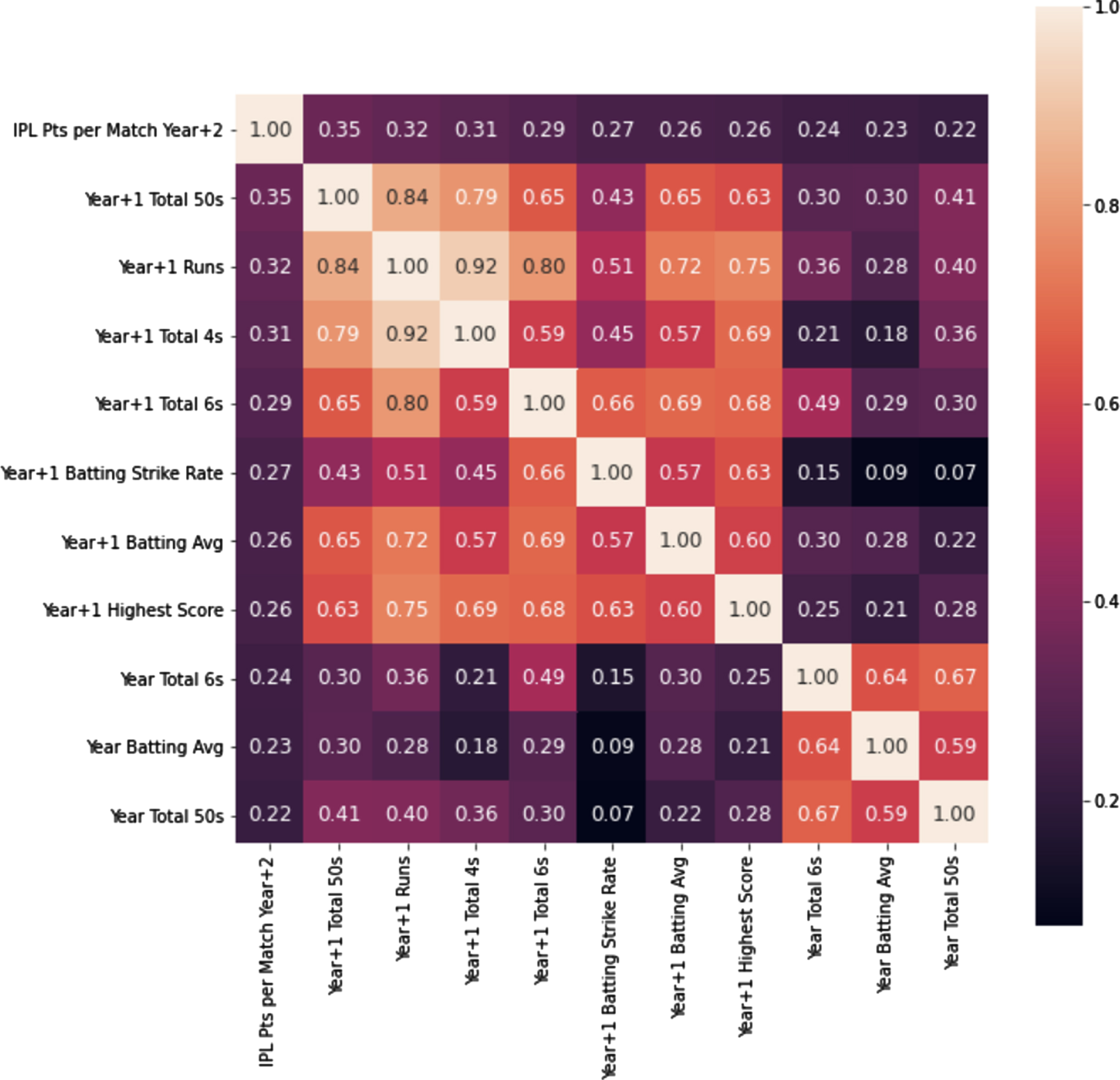
Fig.4
Correlation heatmap of bowler variables used in the ML model.
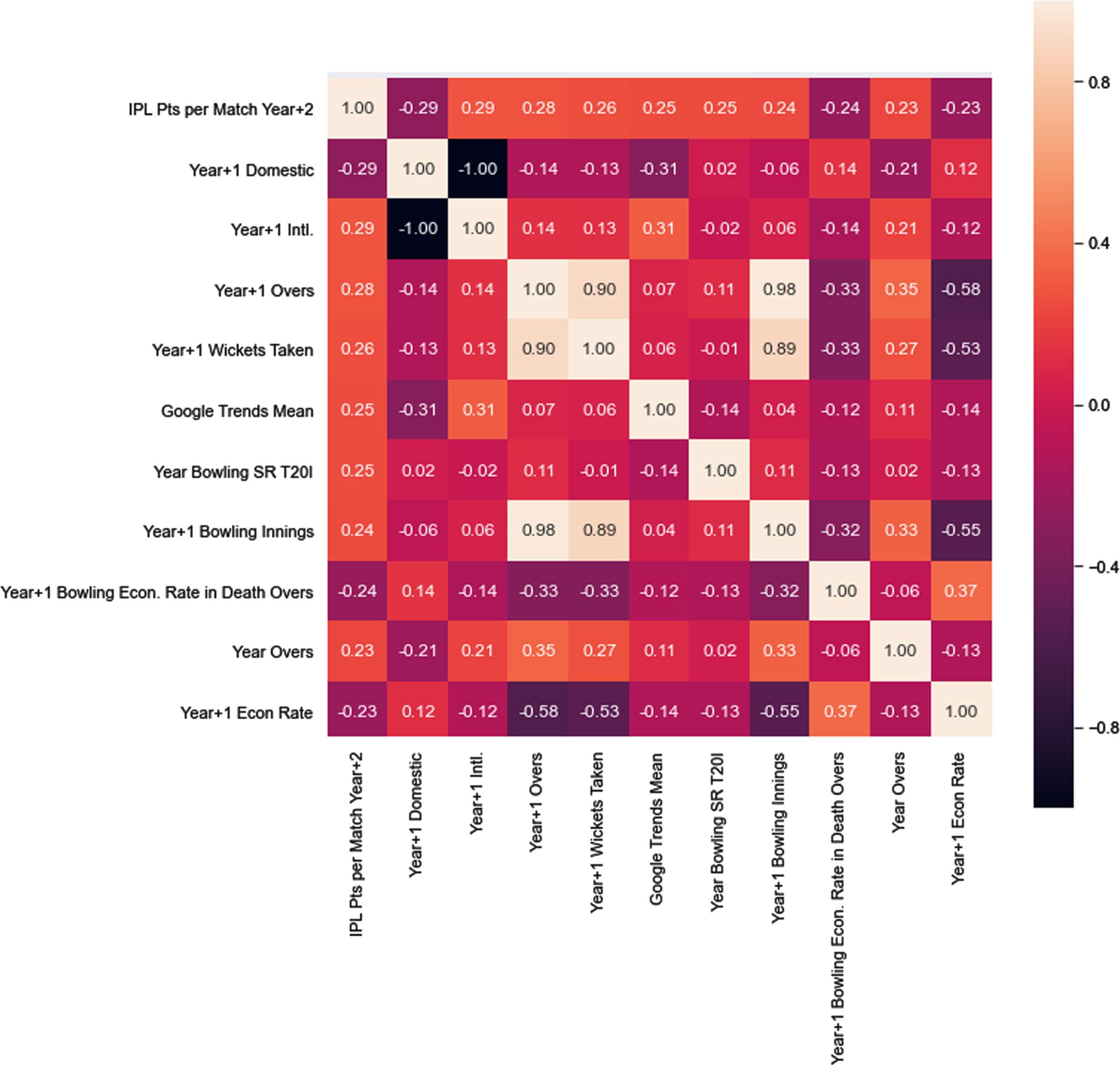
Fig.5
Correlation heatmap of all-rounder variables used in the ML model.
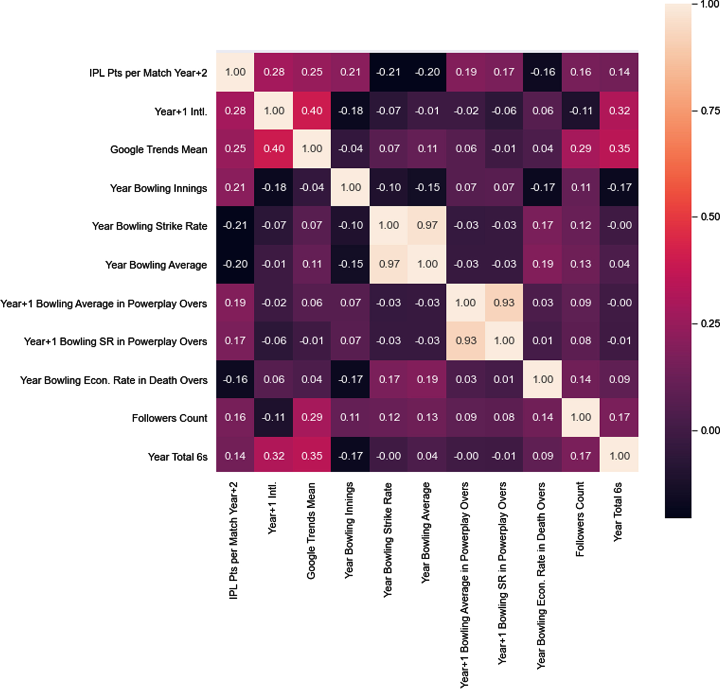
In a correlation heat map, each square in the grid shows the correlation between the variables on each axis. Correlation ranges from –1 to +1. Values closer to zero means there is no linear trend between the two variables. The closer to 1 the variables are more strongly and positively correlated, that is as one variable increases so does the other. Similarly, as correlation approaches –1, the variables are more strongly, but negatively correlated, therefore, as one variable increases the other decreases. The diagonals are all white because those squares are correlating each variable to itself, so it’s a perfect correlation. Therefore, these correlation heat maps were used to eliminate any variables that were highly correlated with each other and choose those that are only highly correlated with the dependent variable –“IPL Pts per Match Year+2”.
The above correlation heatmaps mainly highlight only the batting and bowling abilities and their correlation with each other as well as the dependent variable.
However, it does not consider factors such as age and domestic vs international. Therefore, the relationship between the other factors –age and domestic vs. international –and salary need to be evaluated to understand the way in which the salary varies with these factors. More importantly, it will create emphasis on the need for such factors as they can potentially influence the salary of the player to a large extent.
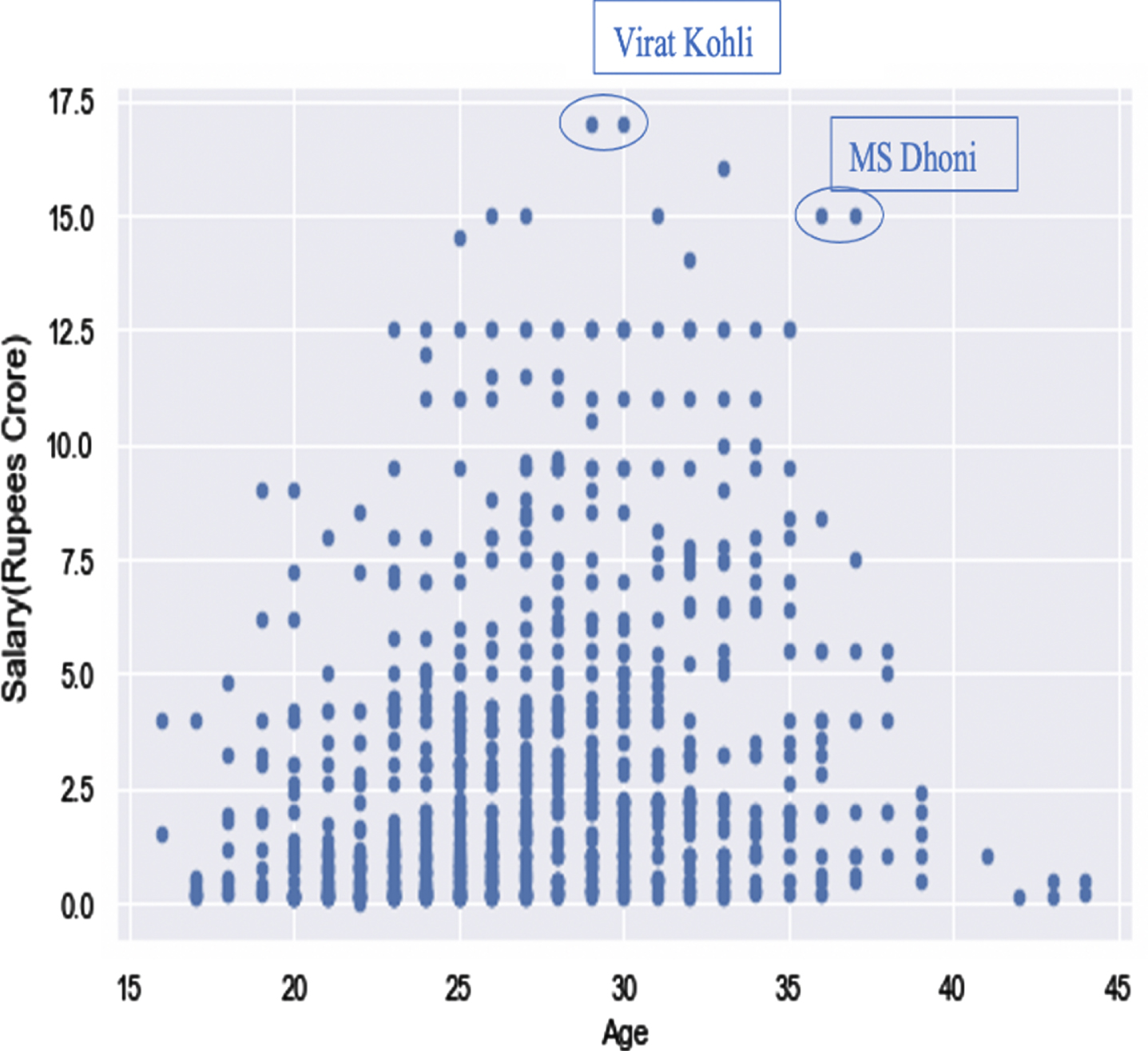
Often, in cricket auctions, there is a trade-off with older players. Apart from having fewer playing years left, seniors are more prone to injury and less agile than younger players. Nonetheless, they are also more experienced, thus often leading to them having icon status23 , and the role of captaincy/leadership. As is evident through Figure 6 and was hypothesized earlier –the correlation between age and agility –the broader trend reflects a bell curve, indicating that players get rewarded for experience up to the peak of around the age of 30), after which age takes a toll on their agility, and ultimately, performance.
Fig. 6
Scatterplot to portray the relationship between Age and Salary (Rupees Crore).
Understanding any meaningful differences or biases in player salaries based on domestic vs international is another important factor in understanding if there are any implicit skews in performance. To analyse this correlation, a master sheet was employed, which contains data across IPL seasons, and to avoid duplicate counting, unique player names were considered. Then, different selections were run on the data frame to output selected and categorized data.
Upon the analysis of possible influence of domestic vs International in performance, it was found that 132 international players played the IPL across the seasons from 2013–2019, while 166 domestic players played in the IPL across the same seasons. Due to the inherent nature of the IPL whose format allows for a very small number of international players in each team, thereby restricting the sample size, it is evident that this variable has quite a significant effect on the valuation of players, therefore, it should be used as a variable to adjust with the format of the IPL.
10Modelling
The underlying assumption that forms the core of this research study is that each player’s economic value is a function of the player’s experience, performance and characteristics (that indirectly contribute to performance). Generalizing the idea of hedonic pricing models24 , the Economic value (EV) of a player (Depken et al., 2010) can be expressed as follows:
The independent variables used as inputs to the function covered a broad array of composite performance factors, the experience levels, and other characteristics such as age, role, and country of origin to holistically assess a player’s value. These inputs are a direct result of the economic impact a player can have, such as through winning games and ultimately tournaments, leading to prize money for the team, or through creating a fan following, thereby generating increased ticket sales for matches. The inputs are likely to be exogenous to the economic valuation of a player to a team, and thus were treated as an explicit function of various inputs.
For the entire predictive modelling process, the players were evaluated differently, depending on their roles. The following are the variables that were used for every category, while the overlapping variables throughout the roles are Age, Role, and Domestic/Intl.
Batsman: Age, Role, Domestic/Intl., Matches, Innings, Not Outs, Runs, Batting Average, Batting Strike Rate, Highest Score, Total 4 s, Total 6 s, Total 50 s, Total 100 s, Batting Average in Death Overs, Batting Strike Rate in Death Overs, Batting Average in Powerplay overs, Batting Strike Rate in Powerplay overs, Batting Average T20I, Batting Strike Rate T20I.
Bowler: Age, Role, Domestic/Intl., Bowling Innings, Overs, Runs Conceded, Wickets Taken, IPL Bowling Average, IPL Economy Rate, IPL Bowling Strike Rate, 4 wickets, 5 wickets, Bowling Average in Death Overs, Bowling Strike Rate in Death Overs, Bowling Economy Rate in Death Overs, Bowling Average in Powerplay Overs, Bowling Strike Rate in Powerplay Overs, Bowling Economy Rate in Powerplay Overs, Bowling Average T20I, Bowling Strike Rate T20I, Bowling Economy Rate T20I.
All-Rounder: Age, Role, Domestic/Intl., Matches, Innings, Not Outs, Runs, Batting Average, Batting Strike Rate, Highest Score, Total 4 s, Total 6 s, Total 50 s, Total 100 s, Batting Average in Death Overs, Batting Strike Rate in Death Overs, Bowling Innings, Overs, Runs Conceded, Wickets Taken, IPL Bowling Average, IPL Economy Rate, IPL Bowling Strike Rate, 4 wickets, 5 wickets, Batting Average in Powerplay overs, Batting Strike Rate in Powerplay overs, Bowling Economy Rate in Death Overs, Bowling Average in Powerplay Overs, Bowling Strike Rate in Powerplay Overs, Bowling Economy Rate in Powerplay Overs, Batting Average T20I, Batting Strike Rate T20I, Bowling Average T20I, Bowling Strike Rate T20I, Bowling Economy Rate T20I.
A data frame –data displayed in a tabular format –containing players for each of these different roles for each IPL season was prepared, and any missing values or anomalies were weeded out. Once the dataset was cleaned and formulated, the data for 2013–2019 years were combined to design a single master sheet. It contained the aforementioned data variables on all the players across the years. This was done due to the insufficient number of players in individual roles for respective years, therefore, with a combined master sheet, it makes it easier to optimise performances of the ML models in terms of accuracy.
Furthermore, in an attempt to obtain a higher accuracy of the ML model, model testing25 and accuracy evaluation was performed not only with these variables, but also their squared values, to discover variables with a stronger relationship with the dependent variable. Moreover, it was an attempt to improve the predictability of the dependent variable with the help of more independent variables. While effort was taken to ensure that the model did not select both the variable and its squared counterpart.
11Checking for multicollinearity –VIR (Variance Inflation factor)
Multicollinearity occurs when independent variables are highly correlated with each other, leading to interdependence between the predictor variables (Frost, 2017). When independent variables are highly correlated to each other, the predictor variable becomes unreliable and loses its significance (Daoud, 2017). Therefore, checking for multicollinearity is an important prerequisite for predictive modelling because of its importance in making sure the independent variables are more reliable.
The Variance Inflation factor (VIF) was used to detect collinearity, after removing the dependent variable and regressing each independent variable against all the others:
The higher the value of VIF, the higher the collinearity, and thus, the higher the sensitivity to small changes and the lesser the precision of the model.
While checking for multicollinearity for this dataset, it was observed that there was a significantly high correlation amongst the independent variables, causing abnormally high VIF values. Effort was taken to reduce it. Thus, for each of the roles, VIF values were calculated for each of the independent variables. Moreover, any values with abnormally high VIF levels or above the tolerance (taken as 50 –determined by the large number of variables) were eliminated and retested.
There were a few instances of structural collinearity in each of the roles. For example, “Year Age” and “Year+1 Age” had perfect correlation (since “Year+1 Age” = “Year Age” + 1) and hence, one of them was removed from the attributes. Ultimately, after testing for collinearity, only those attributes that were below the tolerance level (VIF of 50) were retained.
In most cases though (especially when VIF values exceeded 100), there was data multicollinearity –multicollinearity embedded in the data itself which is difficult to observe –instead of structural multicollinearity –variables that are a by-product and more often than not they are created using an existing variable such as the square of it. And thus, the tolerance was relaxed to accommodate higher VIF values as well, despite the limitation it poses to the accuracy and robustness of the model.
12Machine learning models
The use of ML in applications has grown tremendously over the past decade. The premise of pattern recognition and computers learning through data have helped the computer to be trained in a certain way. Based on the higher data volumes and complex relationships, ML is the obvious choice.
In this use case, in particular, sports analytics, a burgeoning field using machine learning tools, has slowly permeated into every type of sport, such as basketball, baseball, football, and cricket. ML algorithms can be trained to predict data with reasonable accuracy (Das, 2016). Different algorithms have different underlying structures that extend across a vast spectrum: linear, non-linear, tree, probability-based, and combinations of these models (Das, 2016). In this paper, a few have been used to achieve the pre-set objectives of this research study.
However, this research endeavour is inherently different due to the complicated nature of the auction process, team construction, and how players add value to their teams in various domains to ultimately maximize profits for the teams. To avoid the subjectivity and qualitative evaluation of performance in IPL, Machine Learning Models (MLM) were incorporated. Since these use mathematical models, heuristic learning through supervised learning methods, as well as complex decision trees, this provided the robustness and universality needed to ensure the modelling and predictions are reliable and accurate.
The dataset was structured in a standard manner. As a standard measure, 65:35 training data was used throughout the modelling process to test the data. This means that 65% of the dataset were used to train the ML model and the model was tested on 35% of the dataset. For each role, different attributes were selected as independent variables and the dependent variable was universally chosen as the ‘IPL Points’ value of the following season.
The selection of the most reliable, and thus, most accurate ML models among the various options needed to be done. To measure the accuracy of a model, the accuracy metric compares how the observed / actual values differ from the predicted values of the model. One such statistical measure is the R2 metric that varies usually from 0 to 1. However, if the model is tested for out-of-sample data values and/or the mean of the data provides a better fit to the outcomes than the fitted regression outputs, the value can be negative. For this paper, an R2 score was used as a benchmark to compare the performance of each model, because it reflects the percentage of data (or explains the variance around the mean) that is predicted accurately.
13Machine learning models tried and tested
Amongst these models that were designed using Python, linear regression (Lawate et al., 2021) attempts to linearize the relationship between the independent variables and the dependent variable by forming a linear equation. Similarly, Bayesian ridge regression (Srisai, 2016) is a unique dimension to linear regression catering to poorly distributed data that uses probability to formulate linear patterns. Although the R2 scores of Bayesian ridge are similar to the values for linear regression, this model had significant dispersion when the accuracy metric was tested in train and test data. On the other hand, according to literature, Random Forest (Breiman, 2001) has usually tended to be the choice of model due to its ability to explain complex and unstructured relationships with reasonably high accuracy. However, after considering various factors such as simplicity, accuracy, reliability, preference to create an explicit equation such that it can be used easily by inputting the values of the variables, and uniformity across all the roles, linear regression was chosen as the model for all three roles.
Furthermore, after the selection of the model, cross validation was performed. For the model, k-fold cross validation –approximately 5 –was used to ensure that the linear regression prediction model can be generalized to new data, to mitigate problems like selection bias and overfitting (Zhang & Yang, 2015). In addition, for learning algorithms, it is very important to choose appropriate hyperparameters (parameters for a learning process, such as number of features) to not only optimize accuracy but also to prevent overfitting, therefore, hyperparameter tuning was done on the selected model - to determine optimal values of hyperparameters, values that control the process of the model, that would generate the best model output.
14Analysis and results of the study
Using the hedonic pricing idea as a basis, the regression employed on the dataset aimed to maximize accuracy, while also focusing on simplifying the outcome.
Throughout the rest of the research paper, these notations (see Appendix B) will be used to express the variables. The “Year” and “Year+1” are referring to the first and second year of data that is being used as independent variables to predict performance in the following year, for example, “Year+1 Batting Avg” indicates the batting average of the player in the second year, or in other words, one year before the year in which the auction is held - the year for which the estimate auction price is being predicted. In the model results below, since the dependent variable was “IPL Pts per Match”, the model predicts future player performance.
From the table above, it is evident that Random Forest yielded the best results in explaining the underlying variance of the dataset. Research shows that Random Forest algorithms outperform linear modelling approaches. Using feature importance through the decrease in the Gini index (Prakash & Verma, 2022), the model combined k-means clustering and random forest to “accurately determine the relative importance of different features for each role”. This combination of supervised and unsupervised learning approaches enables the model to be more robust in explaining variances in player performances across player roles.
However, it was not used as part of the results because of several reasons: lack of simplicity, not adhering to the basis of hedonic pricing, and because the predictions from the individual trees were in fact correlated to each other, causing overfitting. Moreover, to adhere to the basis of hedonic pricing, while optimizing for R2 values, Linear Regression was chosen.
The following equations have been outputted by the Linear Regression ML model and have been used to predict the performance of players, in terms of points. The coefficients to the variables indicate the relationship of the variable with the predicted performance. For example, a negative coefficient implies a negative relationship between the variable and performance, while a smaller coefficient conveys that it is less significant and it is less of an indicator of performance.
Batsman
5.70 + 0.00126 * Y0BATAVG2 –0.000101 * Y0BATSRP2 + 0.0608 * Y1BATAVGD + 0.569 * Y1WK + 0.211 * Y1T6 –0.000151 * Y0BATAVGD2 –2.68 * Y1T100 –0.00659 * Y1BATAVGP + 0.0181 * Y0BATAVGT20I + 0.000756 * Y1T42 –0.0474 * Y0NO2 –0.000300 * Y0BATAVGP2 –0.590 * Y1NO –0.297 * Y1T50 –0.0801 * Y1D + 1.57 * Y1TOB
R2 score: 0.490
The limitations of this model are the lack of indicators of important aspects such as team characteristics - team chemistry, differing team investments in training, technology and coaches, therefore, such variables that influence a player’s performance were missing and this is responsible for the lower R2 value.
Bowling
9.37 + 0.000709 * Y1BLAVG2 –2.15 * Y1D2 + 0.0747 * Y0BLSRT20I + 0.00185 * Y1A2 + 1.89 * Y1M –0.0419 * Y0BLSR –0.000412 * Y1BLAVGD2 + 0.0539 * Y1BLAVGT20I + 0.0311 * Y0BLAVGD –0.0712 * Y1BLAVG –0.000623 * Y1BL5 W + 0.27896 * Y0BL4W2 –0.000279 * Y1BLAVGP2 + 0.0166 * Y0BLSRP
R2 score: 0.647
All-Rounder
15.0 + 0.000402 * Y1BLAVG2 + 0.0459 * Y0BATAVGP –0.00164 * Y1BLAVGD2 + 0.0312 * Y0BLAVGP –0.00100 * Y0BATAVG2 –0.0291 * Y0BLAVG –0.107 * Y1BLECONT20I + 0.0179 * Y1NO2 –0.0643 * Y0BATAVGT20I –0.0154 * Y1BATSRD –0.193 * Y0BLECONP + 0.448 * Y04 W + 3.07 * Y1INTL2 + 0.00406 * Y0BATSRD + 0.0554 * Y1BOWI –0.00194 * Y1T42 –0.0852 * Y1BLECOND
R2 score: 0.596
15Monetisation: Converting player points into monetary values
Since this model predicts player performance (IPL Pts per Match), it needs to be converted to monetary salary values before actual salary values can be compared with predicted values to elicit any insights on the over- and under-payment of players.
To this end, the following procedure was adopted for each role:
1. The Predicted IPL Points for all the players were standardised using the following formula:
2. Evaluating the difference between the Standardized IPL Points prediction and the minimum value of the standardized predicted values.
3. The minimum salary for all the roles was set to 🙼10,00,000, as this is the minimum auction price for any player in the IPL.
4. Using the budget available to buy players for that specific role and the number of players to be selected, based on the conception for the ideal team, the average player salary was calculated.
5. To convert predicted points into salary, RsPerPoint, a measure to express monetary value for every IPL point in the upcoming season, was calculated using the formula:
6. The predicted salary was then formulated by using the formula:
This essentially assigns a salary of 🙼10,00,000 to the player that is predicted to have the worst performance for each role.
Once the predicted salary values were computed, the difference percentage, a metric to evaluate the deviation, was calculated for each player, each role, and every season, to compare the actual and predicted salaries.
This metric was used throughout the analysis to investigate player valuations.
Tables 3–6 set out to present several statistics about the “Difference Percentage” metric respective to the roles. Moreover, they are presented to aid in the investigation of underpayment and overpayment respective to roles, which will therefore create an emphasis on the purpose of this research study as it strives to bridge the gap between price paid and performance in monetary terms. In addition, a difference percentage metric reflects overpayment if positive and underpayment if negative.
Table 3
Summary Statistics of different types of Bowlers across formats
| Fast | Medium | Spin | ||
| Match | Bowling Average | 44.4 | 39.6 | 44.3 |
| Bowling Econ Rate | 8.9 | 8.0 | 8.3 | |
| Bowling SR | 29.4 | 27.2 | 32.4 | |
| Powerplay Overs | Bowling Avg Powerplay | 40.8 | 31.8 | 22.3 |
| Bowling SR Powerplay | 32.4 | 26.2 | 16.6 | |
| Bowling Econ Rate Powerplay | 7.6 | 7.3 | 8.2 | |
| Death Overs | Bowling Avg Death | 24.6 | 24.3 | 18.9 |
| Bowling SR Death | 13.6 | 14.9 | 11.9 | |
| Bowling Econ Rate Death | 11.0 | 9.5 | 8.5 |
Table 4
ML Models and their R2 scores for Batsman, Bowler and All-Rounder
| ML Model | Batsman R2 score | Bowler R2 score | All-Rounder R2 score |
| Linear Regression | 0.690 | 0.647 | 0.796 |
| Lasso Regression | 0.362 | 0.085 | 0.468 |
| Bayesian Ridge | 0.486 | 0.629 | 0.602 |
| Decision Tree | 0.401 | 0.444 | –0.0985 |
| Random Forest | 0.885 | 0.939 | 0.934 |
| XGBoost | 0.476 | 0.8177 | 0.711 |
Table 5
The overall summary of statistics
| Batsman Difference | Bowler Difference | All Rounder Difference | |
| Percentage (%) | Percentage (%) | Percentage (%) | |
| count | 119 | 84 | 106 |
| mean | 2.7 | –50.4 | –83.06 |
| std | 208.6 | 257.89 | 386.39 |
| min | –2058.42 | –1149.54 | –2416.65 |
Table 6
Top 10 overpaid players (2013–19) –these players created economic deficit
| Player Name | Mean Difference |
| Percentage (%) | |
| DW Steyn | 85.3 |
| Lasith Malinga | 83.5 |
| VR Aaron | 83.4 |
| SP Narine | 82.9 |
| F du Plessis | 80.4 |
| MS Dhoni | 80.3 |
| RG Sharma | 78 |
| TA Boult | 76.5 |
| SK Raina | 75.6 |
| Yuvraj Singh | 64.1 |
As shown in the tables, it is evident that batsmen were, on average, overpaid –with 2.7% of mean difference percentage (see Table 5) –while bowlers and all-rounders tended to be underpaid –with –50.4% and –83.06% of mean difference percentage respectively (see Table 5). The priority on acquiring batsmen in auctions drives this pattern and reiterates the popular saying that T20 cricket is a batsman’s game as explained before. However, it is surprising that all-rounders were, on-average, underpaid; after all, all-rounders tend to add maximum utility to a T20 match. They are not only useful as batsmen in the death overs, considering the batsman order and that crucial runs need to be scored to reach a larger total, but also as bowlers in death overs to restrict runs and build pressure on the opposing team by taking wickets.
As portrayed in Tables 6 and 7, there were large deviations between actual salary and predicted salary as implied by the large absolute mean difference percentage values, for example, it goes up to 85.3% and as small as –2035.7%. Therefore, further investigation was conducted to understand the reasons for the under-payment and the over-payment of players by examining the dynamics of how players were compensated for their experience, with one of them being the age of each player –used as a quantitative proxy value for experience. Figure 7 below shows a polynomial fitted line to highlight the relationship between Age (experience) and the mean difference percentage (%) in predicting the salary of the player.
Table 7
Top 10 underpaid players (2013–19) –These players created economic surplus
| Player Name | Mean Difference |
| Percentage (%) | |
| S Gopal | –2035.7 |
| Bipul Sharma | –1241.3 |
| Sreenath Arvind | –1076.3 |
| Albie Morkel | –913.3 |
| YS Chahal | –720.5 |
| Anureet Singh | –643.8 |
| P Suyal | –513.4 |
| AD Russell | –457.4 |
| PV Tambe | –376 |
| HV Patel | –298.9 |
Fig. 7
Relationship between experience and valuation.
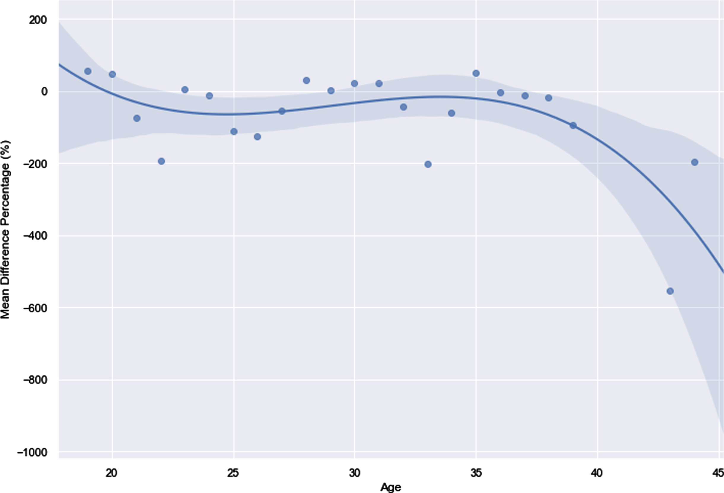
Each turning point in the graph below underscores an interesting complex pattern. With regards to players aged in the early 20 s, teams tended to select young, agile and active players less prone to injury, thus prioritizing proneness to injury over experience and track record. Around the age of 25, the popularity of the player and its accrued marketing benefits would lead to teams paying a premium for such players, despite the decline in agility. However, post the age of 35 for players, teams and auctioneers would not be willing to make high payments for such players, due to their reduced agility and the potential risk of injury. Most of the factors discussed above, i.e. popularity, were considered and identified as an independent variable to the ML model as well.
As expected, the most overpaid players in the graph above tended to be “icon” players, such as KL Rahul who was sold at a whopping 11 crore in the IPL Auction 2018, suggesting they earned more than what their performance and other characteristics yield.
Across seasons and teams, there was a trend of paying a premium rate to famous players. This shows how the popularity of a player generates economic value to a team by increasing fan following and viewership, and as a consequence, marketing benefits. Therefore, it still makes sense for the teams to pay such “icon” players at a premium from an economic standpoint.
To investigate this further and quantify this correlation, social media activity analysis was conducted. Data was scraped across Instagram, Facebook, and Google Search activity, and then aggregated to evaluate the popularity of each player in order to determine its correlation with overpayment, and if applicable, performance. For the analysis, a measure of popularity was constructed by factoring in the Instagram follower count data and Google Trends Index. Due to a high degree of collinearity in data from Facebook, it was not included in the composite weighting. Because the data point values of the player’s Instagram followers and Google Trends index were on completely different scales, data were standardised after combining the values to model the data to a standard normal distribution for ease of analysis and comparison.
It is important to point out that data scraping was constrained by privacy restrictions, as Instagram and Facebook did not allow statistics on a particular data or year to be obtained. Therefore, only the latest data on the followers’ count were available; in this study, data as of 26th December 2020 were used.
The trend is clear: popular players like Virat Kohli, MS Dhoni, Rohit Sharma, Yuvraj Singh, amongst others, were generally overpaid (high positive values), while those on the left side of the mean of the normal distribution of popularity (in a bell curve) tended to be underpaid on average. In a few instances, the absolute value of the Mean difference percentage (%) was predicted to be abnormally high, which then highlighted the great significance of popularity in valuation of the players. In the underpaid category (low negative values), it was observed that star uncapped26 players performed exceptionally well predominantly, which may be because an uncapped player strives to prove himself to get into the national team. However, due to a lack of credibility and a consistent track record, they were not paid well at auctions, and thus, were undervalued. This remains beneficial to the team as they were able to get more utility from the player compared to the money spent on him.
Moreover, often in IPL seasons, anomaly performance displays in bowling or batting skewed the entire regression model parameters, leading to anomalies. While the anomalies present in the dataset would have resulted in a fall in the accuracy metric of the ML model, effort was taken to remove such anomalies from the dataset, which was then trained and tested by the model to increase its reliability.
16Investigating the auction efficiency through economic surplus / deficit
While overpayments and underpayments have been considered and the difference between the actual auction price and the price the player deserved (which was calculated by the ML Model as explained above) were evaluated, another important metric for investigating the IPL’s auction efficiency is to evaluate the surplus or deficit created by a player in a given season. Simply put, this aspect measures the value created (actual performance translated into monetary terms) vs the actual auction price paid, understanding whether player performance justified their auction price in a given season. This further helps to analyse the extent to which there was a misallocation of the budget during the auction, which can prove the inefficiency in the system of valuing the IPL players by the franchises.
Table 10 shows that batsmen tended to, on average, create deficits, thus implying that they were paid more than the monetary value of their individual value creation for the team. Bowlers and all-rounders, on the other hand, tended to, on average, create economic surpluses. All-Rounders created a significant surplus of 38.4% on average across seasons, hence reiterating the notion established in the earlier parts of the research paper that all-rounders were often disproportionately neglected and not adequately paid. At the same time, the table also shows that the All-Rounders tended to have the most variability in predictions, with the standard deviation of 2.86 across seasons. However, teams still prefer investing in batsmen because it’s a batsman’s game in this limited over format of cricket to hedge their bets and to protect themselves against downside exposure.
Table 10
Surplus/deficit created by the players (in %) respective to auction price
| Batsmen | Bowlers | All-Rounders | |
| Average | –14.4% | 21.3% | 38.4% |
| Min | –93.8% | –95.7% | –96.9% |
| Max | 1610% | 950% | 1780% |
| Std. Deviation | 1.69 | 1.91 | 2.86 |
17Assumptions of the study
This research study was based on the following assumptions:
First, in the IPL auction design, an important consideration in the ultimate value of the player is the game-theoretic nature of negotiations between auctioneers, especially during bidding wars, which can often lead to unnecessary economic deficits. This will result in sub-optimal budget allocation by teams due to over- and under-payments at times, which is because of the game theory strategies that come into play in real time.
Often, during auctions, players have their respective base prices: this adds an extra layer of rigidity to the free labour market we had assumed in the model design. This would not only skew the value of a player in a certain direction, but also lead to players remaining unsold (if the base price is too high).
Another feature inherent in the auction design that can lead to inefficiencies is the sequence of players presented in the auction. Often, towards the end of auctions, teams have adequately filled up their squads, or are out of budget to acquire more players. As a result, players presented in the end tend to have less demand, and thus, tend to be underpaid. Hence, this will result in an inefficient allocation of the budget.
Moreover, quite often, especially in transactions involving uncapped players that teams believe have huge potential, teams acquire that player so they can retain the player, nurture him to extract performance and results for the team. An interesting quote captures this idea: “What we assume that the teams should know, but never seem to get, is that you’re paying for the future, not the past” (Akiyanova, 2020). Therefore, this causes under-payment in the short run but greater economic value creation by the player in the long run.
18Conclusion
This research study has generated a model for calculating the valuation of IPL players in a more accurate fashion, with more data points across seasons and cricket formats, along with determining the surplus and deficit of players that has cumulatively investigated the efficiency of the IPL Auctions. The results presented in this research paper highlight the predictive value of such data-driven approaches. Moreover, the Linear Regression - machine learning algorithm - that has been designed in this research study and its results, which highlight large deviations between true performance and actual price paid, show the inadequacies of the valuation of players in the IPL auction, therefore, emphasizing the importance of this research study and its objective.
There are several aspects of the methodology that make it stand out. In the methodology, various iterations were performed for feature selection (variables) that have significant influence on the performance of a player in points. This research study has devised a unique and logic-based method to monetize predicted performance points of a player that were derived through predictive functions - giving an economic value to performance.
While scouring through literature (Prakash et al., 2016; Deep et al., 2016), it was enlightening to see similar research in this domain. However, when the results were back tested against these models, the results appeared to be slightly different at a statistically significant level (0.05 significance level), and the model presented in this paper explains more percentage of the variance as compared to the other models. This could be due to the difference in approach: this model incorporated a wider set of data across seasons, formats, and situations.
Table 8
Average difference percentage (in %) by role and year
| 2015 | 2016 | 2017 | 2018 | |
| Batsman | 22.94 | 5.07 | –48.53 | 32.92 |
| Bowler | –8.79 | –86.4 | –123.38 | 16.85 |
| Allrounder | –2.73 | –144.94 | –148.41 | –12.35 |
Table 9
Mean difference percentage by year and popularity by descending order
| Player | Popularity | Mean Difference |
| Name | Index | Percentage (%) |
| V Kohil | 11.08 | 67.58 |
| MS Dhoni | 6.28 | 8033 |
| RG Sharma | 5.32 | 72.83 |
| Yuvaraj Singh | 5.08 | 64.15 |
| SPD Smith | 5.08 | 46.04 |
| AB de Villiers | 5.02 | 37.96 |
| SK Raina | 5 | 75.63 |
| KL Rahul | 4.98 | –2.92 |
| CH Gayle | 4.95 | 17.09 |
| DA Miller | 4.94 | 48.86 |
The key observations were that the batsmen were (on average) overpaid while bowlers and all-rounders tended to be underpaid. This reiterates the popular belief that T20 is a batsman’s game. Another interesting pattern that emerged from the analysis was regarding the players’ age and popularity as a factor. Teams were more inclined to select young, agile and active players between the age of 25–35, the sweet spot, because these players had little experience and were less prone to injury. Icon players, the popularity index and ability to pull crowds and advertisements also played a significant role in determining a player’s salary and has a lot of premium from an economic standpoint. The calculation of economic surplus/deficit also pointed in the same direction as mentioned earlier, that the batsman tended to, on average, create deficits, implying that they were paid more than the monetary value of their individual value creation for the team, while bowlers and all-rounders, on an average, created economic surpluses.
Throughout the research, given the complex nature of the relationship, the investigation was not only explored from a purely quantitative perspective, other behavioural and psychological factors such as economic value creation for teams, marginal utility of players in teams, and the game-theoretic design of auctions, involving bid and offer dynamics, typical to hedonic pricing mechanisms, were also explored and considered. In addition, the research findings also consider the profit-maximizing motives of the IPL franchises such as maximizing revenue collected from ticket sales, and these motives are the reason for buying Icon players like Virat Kohli and Rohit Sharma, as they attract spectators due to their large fan following.
In conclusion, the model developed in this research study could serve as a benchmark for valuations of players in IPL and further facilitates the incorporation of quantitative methods in other sports and formats alike to ensure the improved compatibility between compensation and player performance.
Moreover, the unique prescriptive analytics approach to this multi-dimensional problem of predictive sports performances highlights the need for broader and more holistic modelling processes in sports analytics, a domain that has been under-researched and overlooked. While the hedonic method of pricing players in sports analytics is not unique to this paper, it reflects the significance of this method to understand how each variable interacts with the player performance index to ultimately understand embedded patterns in players’ performances. Ultimately, to make such analytical models for cricket more robust, further research is needed across more alternative data points and quantification of behavioural aspects of the game such as Law of Averages, salary as an incentivizing function, amongst others, to improve the accuracy of the model in predicting future player performances, and thus optimal salaries.
Acknowledgments
The author would like to express special thanks to mentor, Mr. Pramod Krishnamurthy (an IIT and IIM Calcutta alumnus, having wide knowledge and expertise in Sports Analytics with total 30 years of experience, ex-CEO SportsQ and ex-CTO Birla Sun Life Insurance) for the patient guidance, support, and invaluable encouragement he has provided since the beginning. He has been a guiding force throughout the research journey, whether through directing me, offering feedback and sharing ideas throughout the modelling process, and connecting with different experts in the sports analytics field. The author would like to express sincere gratitude for the knowledge shared along with the time spent during the project.
The author would also like to sincerely thank Mr. Maheshwarran Karthikeyan (a data scientist and a cricket enthusiast who has worked in GyanData) who has also offered insights during this project. His knowledge and his exemplary passion in this domain have helped to conduct this research investigation effectively, and in a structured manner. They have also enabled to improve research capabilities and develop higher-order thinking skills.
Supplementary material
{ label (or @symbol) needed for fn } The Appendix is available in the electronic version of this article: https://dx.doi.org/10.3233/JSA-200580.
References
1 | Ahmed F. , Deb K. , Jindal A. 2013. Multi-objective opti1mization and decision making approaches to cricket team selection. |
2 | Akiyanova A. , 2020. Changing the game: How data analytics is upending Baseball, Upenn.edu. Available at: https://wsb.wharton.upenn.edu/changing-the-game-howdata-analytics-is-upending-baseball/ (Accessed: March 23, 2021). |
3 | Boyle T. , Hyperparameter Tuning. [online] Medium. Available at: <https://towardsdatascience.com/hyperparametertuning-c5619e7e6624> [Accessed 22 February 2021]. |
4 | Chakraborty A. , 2021. CORRECTED-ANALYSISCricket-Indian Premier League cash-cow delivers even in COVID times. [online] U.S. Available at: <https://www.reuters.com/article/cricket-ipl/correctedanalysis-cricket-indian-premier-league-cash-cow-deliverseven-in-covid-times-idUSL4N2I101J> [Accessed 22 February 2021]. |
5 | Cricinfo, 2021. Champions League Twenty20 Cricket Team Records & Stats | ESPNcricinfo.com. [online] Available at: <https://stats.espncricinfo.com/ci/engine/records/team/seriesresults.html?id=120;type=trophy> [Accessed 18 January 2021]. |
6 | Chopra A. , 2021. Why teams are slower off the blocks but are scoring faster than ever at the death. [online] ESPNcricinfo. Available at: <https://www.espncricinfo.com/story/ipl-2020-aakash-chopra-why-teams-are-slower-to-get-off-theblocks-but-scoring-faster-than-ever-at-the-death-1235918> [Accessed 18 January 2021]. |
7 | Daoud J.I. , Multicollinearity 2017. 2017. Multicollinearity and regression analysis, Journal of Physics Conference Series 949, 012009. |
8 | Das S. , 2016. [online] Srdas.github.io. Available at: < https://srdas.github.io/Papers/DSABook.pdf> [Accessed 18 January 2021]. |
9 | Davis J. , Perera H. , Swartz T. n.d. Player Evaluation in Twenty20 Cricket. [online] Available at: <https://www.sfu.ca/tswartz/papers/moneyball.pdf> [Accessed 15 November 2020]. |
10 | Deep C. , Patvardhan C. , Singh S. A new machine learning based deep performance index for ranking IPL T20 cricketers, International journal of computer applications. 137: (10) ((2016) ), 42–49. |
11 | Depken C.A. , Rajasekhar R. 2010. Open market valuation of player performance in cricket: Evidence from the Indian premier league, SSRN Electronic Journal. doi: 10.2139/ssrn.1593196. |
12 | Eapen J. , 2021. Can IPL’s Season 13 match Season 12’s record popularity? – YouGov Sport. [online] Sport.yougov.com. Available at: <https://sport.yougov.com/can-ipls-season-13-match-season-12s-record-popularity/> [Accessed 22 February 2021]. |
13 | ET Bureau., 2017. IPL teams to spend up to Rs 640 crore on players in 2018, Economic Times. Available at: https://economictimes.indiatimes.com/news/sports/eachfranchise-can-secure-5-cricketers-for-ipl-2018/articleshow/61947178.cms (Accessed: March 23, 2021). |
14 | Frost J. , 2017. Multicollinearity in regression analysis: Problems, detection, and solutions - statistics by Jim, Statisticsbyjim.com. Available at: https://statisticsbyjim.com/regression/multicollinearity-in-regression-analysis/ (Accessed: November 13, 2020) |
15 | Herridge R. , Turner A.N. , Bishop C. 2017. Monitoring Changes In Power, Speed, Agility And Endurance In Elite Cricketers During. |
16 | The Off-Season, Journal of Strength and Conditioning Research. Available at: https://www.researchgate.net/publication/317972599_Monitoring_Changes_In_Power_Speed_Agility_And_Endurance_In_Elite_Cricketers_During_The_Off-Season (Accessed: November 13, 2020). |
17 | Importance Of Cricket (Game)., 2016 Gen.in. Available at: http://pune.gen.in/india/importance-cricket-game/607/(Accessed: March 21, 2021). |
18 | Breiman L. , 2001. Random forests –machine learning. SpringerLink. Retrieved April 22, 2022, from https://link.springer.com/article/10.1023/A:1010933404324>. |
19 | IPLT20.Com - Indian premier league official website (no date) Iplt20.com. Available at: https://www.iplt20.com/about/code-of-conduct-for-players-and-team-officials (Accessed: November 25, 2020). |
20 | Kalechofsky H. , 2016. A Simple Framework for Building Predictive Models. Available at: https://www.msquared.com/wp-content/uploads/2017/01/A-Simple-Framework-for-Building-Predictive-Models.pdf (Accessed: October 12, 2020). |
21 | Karnik A. , 2010. Valuing cricketers using hedonic price models, Journal of Sports Econ. Available at: https://www.researchgate.net/publication/227359953ValuingCricketersUsingHedonicPriceModels (Accessed: September 14, 2020). |
22 | Klemperer P. , Auctions: 2004. 2004. Auctions: Theory and practice, SSRN Electronic Journal. doi: 10.2139/ssrn.491563. |
23 | Kohli B.Y.R. , 2009. The launch of the Indian premier league, Columbia.edu. Available at: https://www0.gsb.columbia.edu/mygsb/faculty/research/pubfiles/5179/IPL.pdf (Accessed: October 23, 2020). |
24 | Levin J. , 2004. Auction Theory, Stanford.edu. Available at: https://web.stanford.edu/jdlevin/Econ%20286/Auctions.pdf (Accessed: October 23, 2020). |
25 | Mitra, S. , The 2010.IPL: India’s foray into world sports business, Sport in society. 13: (9), 1314–1333. |
26 | Mittal A. , Manavalan A. 2017. The IPL model: Sports marketing and product placement sponsorship, Ijhssi.org. Available at: http://www.ijhssi.org/papers/v6(2)/version-4/H0602044461.pdf (Accessed: November 19, 2020). |
27 | Perez L.V. , 2017. Principal component analysis to address multicollinearity, Whitman.edu. Available at: https://www.whitman.edu/Documents/Academics/Mathematics/2017/Perez.pdf (Accessed: March 19, 2021). |
28 | Rastogi S.K. , Deodhar S.Y. Player pricing and valuation of cricketing attributes: Exploring the IPL Twenty20 vision, Vikalpa The Journal for Decision Makers. 34: (2) ((2009) ), 15–24. |
29 | Singh S. , Gupta S. , Gupta V. 2010. Dynamic bidding strategy for players auction in IPL, Worldacademicunion.com. Avail1able at: http://www.worldacademicunion.com/journal/SSCI/sscivol05no01paper01.pdf (Accessed: March 12, 2021). |
30 | Zhang Y. , Yang Y. Cross-validation for selecting a model selection procedure, Journal of Econometrics. 187: (1) ((2015) ), 95–112. |
31 | Prakash C.D. , Patvardhan C. , Lakshmi C.V. 2016. Data Analytics based Deep Mayo predictor for IPL-9. IJCA. Retrieved April 30, 2022,from https://www.ijcaonline.org/archives/volume152/number6/26321-2016911875. |
32 | Prakash C.D. , Verma S. 2022. A new in-form and role-based deep player performance index for player evaluation in T20 cricket. Decision Analytics Journal. Retrieved April 30, 2022, from https://www.sciencedirect.com/science/article/pii/S2772662222000029 [Accessed 30th April 2022]. |
33 | Lawate A. , Katare N. , Hoskeri S. , Takle S. , 2021. Cricket analysis and prediction of projected score and winner using machine learning. International Journal of Advanced Research in Computer and Communication Engineering. Retrieved March 30, 2022, from https://ijarcce.com/u%2016/IJARCCE%2015.pdf. |
34 | Srisai S. , 2016. A Bayesian stochastic model for team performance evaluation in T20 cricket: Effectiveness of Power Hitting&Consistency. A bayesian stochastic model for Team Performance Evaluation in T20 cricket: Effectiveness of power hitting & consistency. Retrieved April 30, 2022, from https://srisai85.github.io/T20Cricket/BayesiananalysisofT20Cricket.html. |
Notes
1 A short cricket match with 20 overs of gameplay per innings,
2 A one-day international with 50 overs of gameplay per innings
3 Usually 5-day cricket game and each day at least 90 overs are bowled.
4 A set of games played after the regular season by the top 4 competitors to determine the league champion
5 Law of Averages (Gambler’s fallacy) –The number of events deviating from the long-term average of a player must balance out across seasons and matches.
6 Batters who bat first in the batting innings (#1 or #2)
7 Batters who come #3 and #4 in the batting innings.
8 Batters #5, #6, #7, or #8 in the batting innings.
9 Rely primarily on speed of the ball to dismiss batsmen.
10 Bowl at slower speeds than fast bowlers (around 90–120 kmph) with other deceptive tactics.
11 Rely primarily on rotation of ball to dismiss batsmen.
12 Cricketer who performs well in batting and bowling.
13 Player on the fielding side who stands behind the wicket being guarded by the batsman currently on strike.)
14 Each of two divisions of a game during which one side has a turn at batting
15 The number of times that a batsman having begun an innings and not be dismissed
16 The highest number of runs scored in an innings throughout the seasons
17 The number of times a batsman has scored 50–100 runs in an innings throughout the season
18 The number of times a batsman has scored 100+ runs in an innings throughout the season
19 10 Experience bias explains the inherent nature of the player performance dataset, which assumes that more number of matches implies more performance.
20 A fielding position behind the batter on the off side of the field.
21 To extract data, APIs, libraries, and web scraper functions were constructed to improve the efficiency of collecting clean, reliable data
22 The supposed principle that future events are likely to turn out so they balance any past deviation from a presumed average.
23 Icon status is often used to denote the most valued player in the team, through their experience and contribution to team performance; however, it is often mistaken for the most popular players as well, which does not necessarily correlate with player performance.
24 They are used to relate the price of a good to the features or inputs that define it.
25 The process in which the performance of a fully trained model is evaluated on a testing dataset.
26 Uncapped player is defined as a player who has not represented his country yet at the international level in any cricket format.


