
Dynamic cricket match outcome prediction
Abstract
To propose a model where match outcome is predicted ball by ball at the start of the second inning. Our methodology not only incorporates the dynamically updating game context as the game progresses, but also includes the relative strength between the two teams playing the match. We used 692 matches from all seasons (2008–2018) to train our model, and we used all 59 matches from the current season (2019) to test its performance. Here we have engineered 11 players and 10 bowlers, and all their metrics are tracked as a function of each ball of each over throughout the match during the second inning, also keeping in the consideration of dynamically changing target score as one of the attributes. Initially, we tried Logistic Regression, Naive Bayes, K-Nearest Neighbour (KNN), Support Vector Machine, Decision Tree, Random Forest, Boosting, Bagging, and Gradient Boosting with an accuracy of 76.47%(+/–3.77%). With deep learning, we tried the various flavours of LSTM and GRU like vanilla, Bidirectional and stacked to train our models and the results found are very impressive with an accuracy of 76.13%(+/–2.59%). All of these flavors were tested using various approaches such as one-to-one sequencing, one-to-many sequencing, many-to-one sequencing, and many-to-many sequencing, which are discussed in this paper. An accurate prediction of how many runs a batsman is likely to score and how many wickets a bowler is likely to take in a match will help the team management select the best players for each match.
1Introduction
Cricket match is a team game which involves two teams each consists of 11 players. The different formats of cricket played are Test match, One Day International and Twenty20.We focus our research on Indian Premier League (IPL) Twenty20s, the most popular format of the game and embark on predicting the dynamic outcome of a Indian Premier League (IPL) cricket match. Twenty20 format consist of 20 overs for each team with 6 balls in each over. An average of three hours is taken to complete both the innings. So this format of match is comparatively shorter than other formats. The Indian Premier League (IPL) is a professional Twenty20 played during months of April and May of every year in India and there may be a minimum of 8 to 10 teams playing where each team plays with remaining all teams for a minimum of two times. Matches are held at different venues under the control of The Board of Control for Cricket in India (BCCI). Toss winning is one of the crucial factor in deciding the winner of the match. Toss winning team can wish to either field or bat. The team batting first we called as first inning and team will try to pose as many runs as possible in 20 overs to set target for the opponent during their second inning. The team batting in second inning need to chase the target in order to win the game with wickets in hand. More details on the data and empirical results are discussed in later sections.
2Related work
C. R. Lamsal and A. Choudhary et al., 2018 proposed multivariate regression based solution where each player playing in the IPL match is evaluated with points based on their past performance and weights are assigned to team represented by them. They identified seven factors which influence the outcome of the IPL match and modelled the dataset based on these factors. V. V. Sankaranarayanan, J. Sattar, and L. V. S. Lakshmanan et al., 2014 build a prediction system that takes in previous old match data as well as live data of the match and predicts the match outcome as win or loss. They applied combination of linear regression and nearest neighbour clustering algorithms to predict the score. S. B. Jayanth et al., 2018 proposed various models using supervised learning method using SVM model with linear, and nonlinear poly and RBF kernels algorithms to predict the outcome of game by considering the batting order of both playing teams. They also propose a model for recommendation of player for any specific role in team based on his historical performances. N. Tandon, A. S. Varde, and G. de Melo et al., 2018 gave brief overview of the state of common sense Knowledge (CSK) in Machine Intelligence provides insights into CSK acquisition, CSK in natural language, applications of CSK and discussion of open issues. This paper provides a report of a tutorial at a recent conference with a brief survey of topics. L. Van den Berg, B. Coetzee, S. Blignaut, and M. Mearns et al., 2018 study indicated that easy available sources are not effectively utilized, data collection processes are not performed in a structured manner and coaches need skill development regarding data collection and analysis. Furthermore, the lack of technology as well as the absence of a person who can collect data and a shortage of skills by the person who is responsible for data collection, are the main challenges coaches face. G. Melo et al., 2015 provide an overview of new scalable techniques for knowledge discovery. Their focus is on the areas of cloud data mining and machine learning, semi-supervised processing, and deep learning. They also give practical advice for choosing among different methods and discuss open research problems and concerns. J. H. Schoeman, M. C. Matthee, and P. Van der Merwe et al., 2006 considers the viability of using data mining tools and techniques in sports, particularly with regard to mining the sports match itself. An interpretive field study is conducted in which two research questions are answered. Firstly, can proven business data mining techniques be applied to sports games in order to discover hidden knowledge? Secondly, is such an analytical and time-consuming exercise suited to the sports world? An exploratory field study was conducted wherein match data for the South African cricket team was mined. The findings were presented to stakeholders in the South African team to determine whether such a data mining exercise is viable in the sports environment. While many data constraints exist, it was found that traditional data mining tools and techniques could be successful in highlighting unknown patterns in sports match data. P. Basavaraju and A. S. Varde et al., 2017 gives a comprehensive review of a few useful supervised learning approaches along with their implementation in mobile apps, focusing on Androids as they constitute over 50%of the global smartphone market. It includes description of the approaches and portrays interesting Android apps deploying them, addressing classification and regression problems. P. U. Maheswari et al, discussed about an automated framework to identify specifics and correlations among play patterns, so as to haul out knowledge which can further be represented in the form of useful information in relevance to modify or improve coaching strategies and methodologies to confine performance enrichment at team level as well as individual. With this information, a coach can assess the effectiveness of certain coaching decisions and formulate game strategy for subsequent games. Kaluarachchi et al.,2010 discussed winning or losing in ODU match whereas we research for IPL matches. There they worked majorly on classical Bayesian classifiers for prediction whereas here we used classical as well as deep neural network to find out the best prediction.
3Materials and methods
3.1Data mining
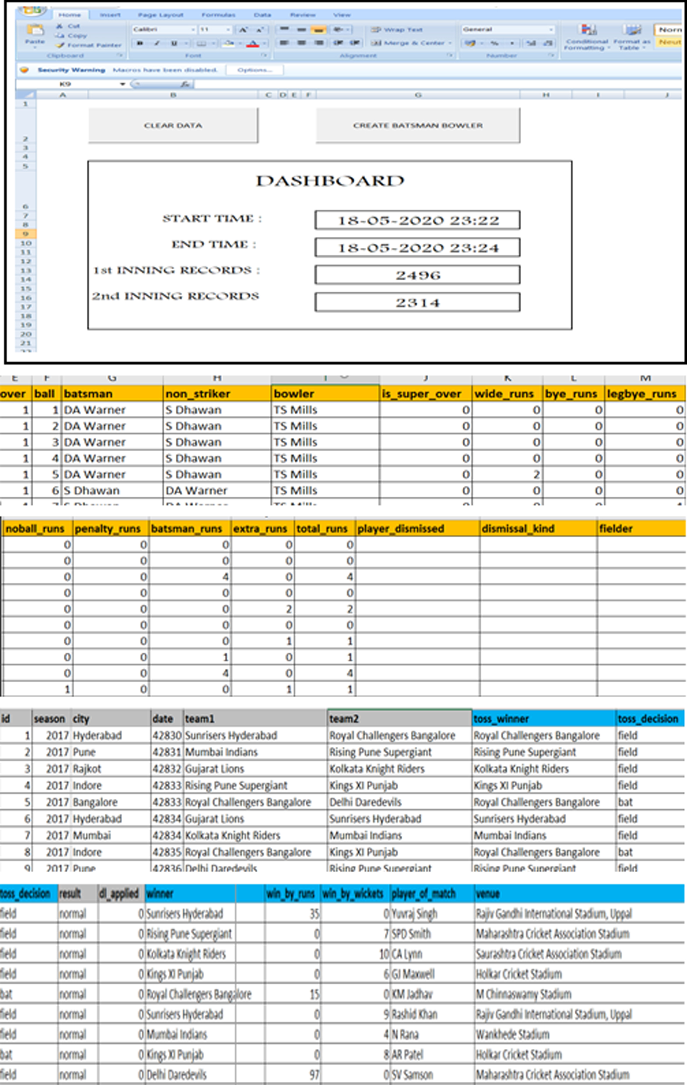
This is different from the earlier techniques that have been implemented in the papers. Most of the research around predicting the match outcome takes into account a lot of different features and only makes one prediction. We have tried to adopt a different approach where we make predictions on the outcome of a match when the second team starts batting. This prediction is in regards to the second batting team and if the team will win or lose based on the match circumstances. Historical matches and player data for the Twenty20 IPL competition was scraped from the archive section of cricket fan site cricinfo.com4 for the seasons 2008 to 2019. This raw data was then cleaned and combined into two datasets for matches and deliveries. From these datasets, features sets are constructed that form the input for our model using automated excel macros. With these two datasets as input we formulated rules in the excel which in turn constructed required features of our interest for all the past Twenty20 IPL matches. The features that we have been constructed to train the model are different from any other set of features that have been used before. Total 90 attributes are created by the excel macros (Fig. 2)
Fig. 1
Exploratory Data Analysis on the constructed features.
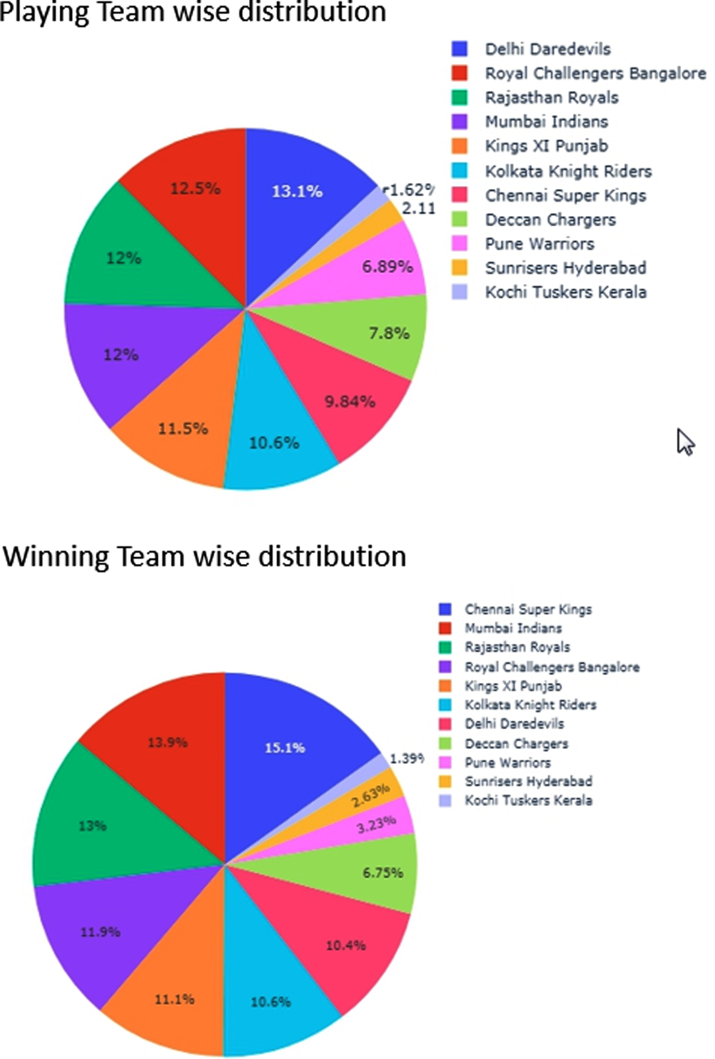
Fig. 2
Excel Macros for features constructions.
3.2Feature selection
All matches from season 2008 to 2018 are used to train our model. This train dataset comprises of 692 matches and approx. 80,000 data points. Test data set we have selected consists of 59 matches of season 2019 and approx. 7,000 data points for prediction. No one has taken before such high data set for their predictions. We have total 90 features, which when fed to the model gives poor results. Such bad performance of the model is due to “Curse of Dimensionality”. The curse of dimensionality is one of the most important problems in multivariate machine learning. The method that we have used for feature selection is wrapper method. Wrapper feature selection methods create many models with different subsets of input features and select those features that result in the best performing model according to a performance metric. These methods are unconcerned with the variable types, although they can be computationally expensive. We identified 30 attributes that best fit to our models. The feature set as shown in Table 1, comprises of our dependent and independent variables. Here “Result” is our target categorical dependent variable. Independent parameters are constructed through excel macros utilities from our available datasets of matches and deliveries. Here we have constructed 11 batsmen and 10 bowlers and all their metrics are tracked as a function of each ball of each over throughout the match during the second inning. Also the “Target” score during the second inning is set as one of the independent attribute which gets updated dynamically as the second inning batting metrics changes as we can see from the table below, these are the final set of feature that are fed to the model. Our input data is first splitted into train dataset and test dataset on the basis of season. Then we perform KFold TimeSeriesSplit on our train dataset to ensure that we have not introduced any bias–variance trade-off in our model. In statistics and machine learning, the bias–variance trade-off is the property of a set of predictive models whereby models with a lower bias in parameter estimation have a higher variance of the parameter estimates across samples, and vice versa. Final predictions are made on the test data and model performance is evaluated.
Table 1
Table showing best fit features fed to the model
| Attributes | Description |
| Match id | The match Id for each match in the IPL |
| Ball | The current order of the ball bowled |
| Over | The current over of the match |
| Balls | Played Balls left to be bowled |
| Bman1 –Bman11 | Runs scored by the batsman on each ball |
| Bowl1 - Bowl10 | Runs scored on every ball bowled by bowler |
| Extra runs | Extras given by bowlers calculated for each ball |
| Batsman runs | Runs scored by batsman on each ball |
| Remaining Balls | The total no of balls left |
| Wickets Left | The total no of wickets left |
| Present Score | Current score |
| Target | Total runs scored by the team batting first |
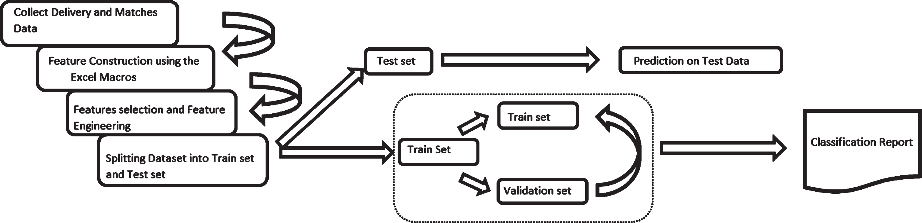
Fig. 3
Architecture of the Model (Flow Diagram).
4Results and discussion
Below table shows notation which we followed for our model nomenclature –
Table 2
Model Nomenclature
| Abbreviation | Description |
| o2o | One to one sequence |
| m2o | Many to one sequence |
| o2m | One to Many sequence |
| o2o | Many to Many sequence |
| MF | Multivariate Feature |
| bidirec | Bidirectional |
| LSTM | Long Short Term Memory |
| GRU | Gated Recurrent Unit |
4.1MODEL 1 (1–20 over)
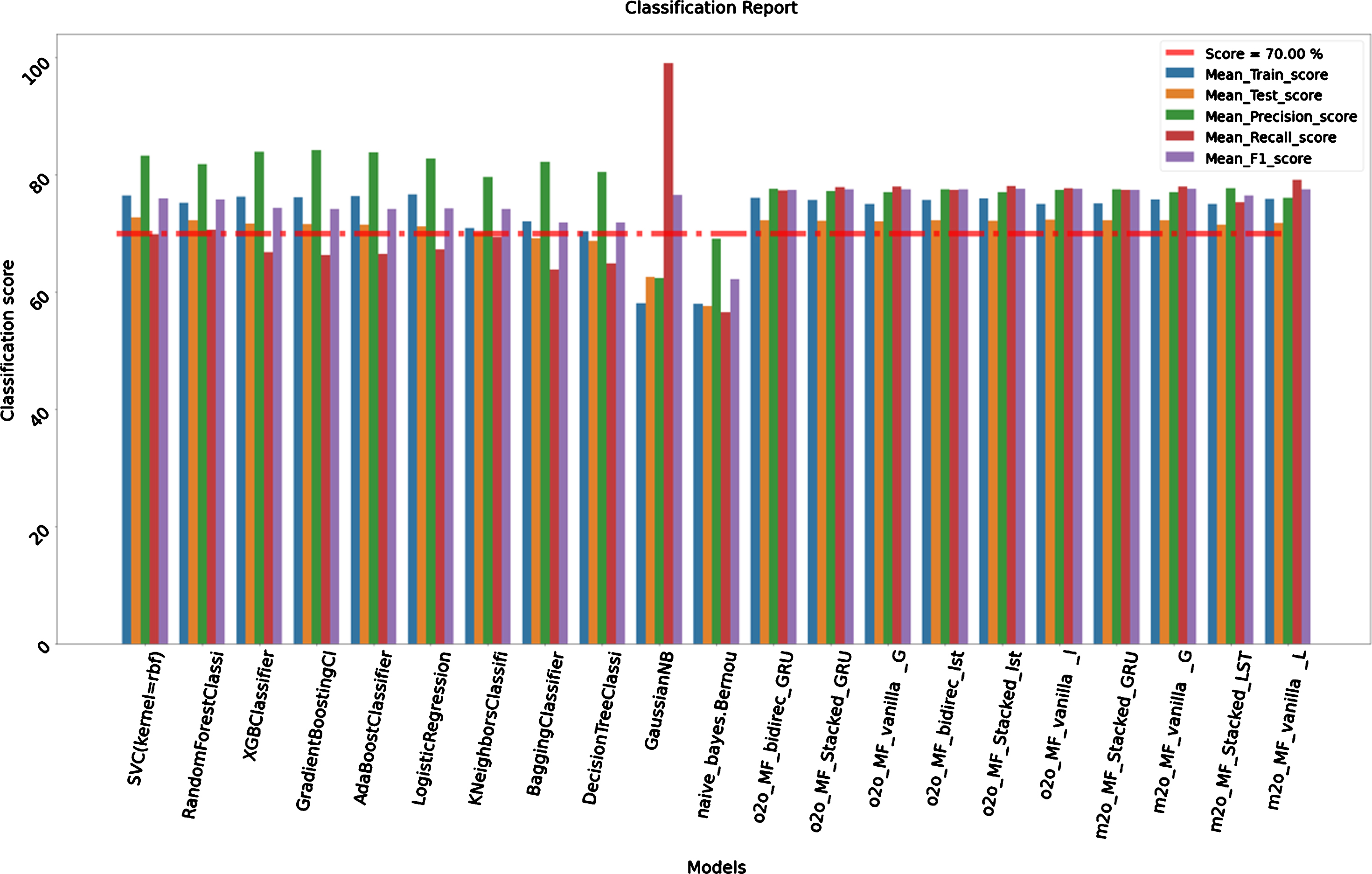
For this model we considered 692 matches of all the seasons (2008–2018) to train our model and all the 59 matches of season (2019) to test it. Train size is 79,129 and test size is 6,960. The comparative classification report given out by the model for all the classical and neural algorithms are provided below in the Table 3. As we can see in the below analysis table, among traditional machine learning algorithms SVC and RandomForestClassifier show very good results. The train accuracies are 76.47 %with confidence interval of 3.77%and test accuracies are 72.74%. Both the models have very high precision of 83.25 %and 81.90%. XGBClassifier also have very high precision of 83.92%. In deep learning models one-to-one sequence vanilla LSTM shows good accuracy of 75.05%with the confidence interval of 3.12%. We can see that the recall score and F1 score of deep learning model are comparatively higher than traditional models which means deep models are better able to classify the classes correctly than traditional models. Gaussian Naïve Bayes and Bernoulli Naïve Bayes shows very less mean train and test scores. This might be due to its assumption that attributes are independent and attributes are continuous in nature. We can see below comparative bar graph (Fig. 4) of these results to have better visualization of performance of each algorithm.
Table 3
Classification report Results (Over 1–20)
| Name | Mean_Train_score | Test_score | Precision_score | Recall_score | F1_score |
| SVC | 76.47%(+/–3.77%) | 72.74% | 83.25% | 69.85% | 75.97% |
| RandomForestClassifier | 75.28%(+/–3.09%) | 72.27% | 81.90% | 70.64% | 75.86% |
| XGBClassifier | 76.34%(+/–3.93%) | 71.67% | 83.92% | 66.87% | 74.43% |
| GradientBoostingClassifier | 76.23%(+/–3.96%) | 71.61% | 84.26% | 66.36% | 74.24% |
| AdaBoostClassifier | 76.40%(+/–3.87%) | 71.49% | 83.88% | 66.57% | 74.23% |
| Logistic Regression | 76.72%(+/–4.13%) | 71.22% | 82.80% | 67.31% | 74.26% |
| KNeighborsClassifier | 70.92%(+/–2.11%) | 70.22% | 79.67% | 69.41% | 74.19% |
| Bagging Classifier | 72.06%(+/–2.88%) | 69.20% | 82.21% | 63.86% | 71.89% |
| DecisionTreeClassifier | 70.41%(+/–2.14%) | 68.71% | 80.55% | 64.93% | 71.90% |
| GaussianNB | 58.15%(+/–2.63%) | 62.66% | 62.42% | 99.11% | 76.60% |
| BernoulliNB | 58.06%(+/–0.60%) | 57.61% | 69.10% | 56.57% | 62.21% |
| o2o_MF_bidirec_GRU | 76.13%(+/–2.59%) | 72.30% | 77.66% | 77.33% | 77.49% |
| o2o_MF_Stacked_GRU | 75.76%(+/–3.01%) | 72.23% | 77.22% | 77.96% | 77.59% |
| o2o_MF_vanilla_GRU | 75.03%(+/–3.01%) | 72.11% | 77.05% | 78.01% | 77.53% |
| o2o_MF_bidirec_lstm | 75.69%(+/–3.02%) | 72.28% | 77.55% | 77.49% | 77.52% |
| o2o_MF_Stacked_lstm | 76.06%(+/–3.04%) | 72.20% | 77.11% | 78.10% | 77.60% |
| o2o_MF_vanilla_lstm | 75.05%(+/–3.12%) | 72.37% | 77.50% | 77.77% | 77.64% |
| m2o_MF_Stacked_GRU | 75.14%(+/–3.63%) | 72.25% | 77.51% | 77.46% | 77.49% |
| m2o_MF_vanilla_GRU | 75.85%(+/–3.16%) | 72.28% | 77.05% | 78.00% | 77.62% |
| m2o_MF_Stacked_LSTM | 75.09%(+/–2.90%) | 71.50% | 77.76% | 75.31% | 76.52% |
| m2o_MF_vanilla_LSTM | 75.94%(+/–3.84%) | 71.80% | 76.08% | 79.16% | 77.59% |
Fig. 4
Graph Classification Report Results (Over 1–20).
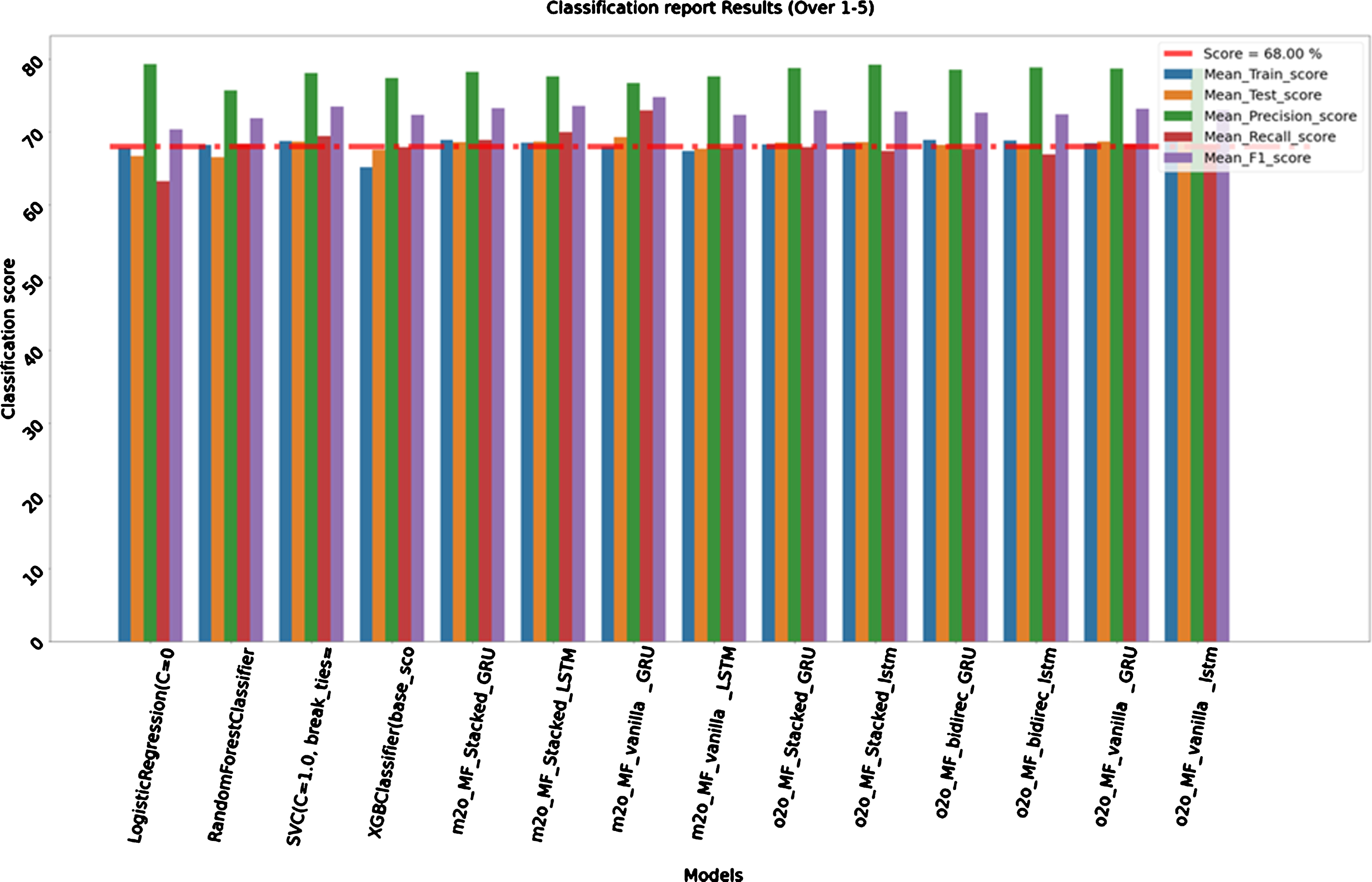
4.2MODEL 2 (1–5 over)
For this model we considered all records from 1 to 5 over of all seasons (2008–2018) to train our model and all 1 to 5 over of seasons (2019) to test it. Train size is 21,662 and test size is 1,820. Here SVC from traditional machine learning family and one-to-one sequence vanilla LSTM from deep learning models shows good results during the start of second inning itself. Below results in Table 4 are from first 5 overs of the second inning. The train accuracies are 68.71%, and 68.89%with confidence interval of 1.90%, and 2.20%and test accuracies of 68.68%, and 68.57%respectively. Logistic Regression is showing exceptionally high precision score of 79.27%. Again below is the comparative bar graph (Fig. 5) of results to have better visualization of performance of each algorithm between 1–5 overs.
Table 4
Classification Report Results (Over 1–5)
| Name | Mean_Train_score | Test_score | Precision_score | Recall_score | F1_score |
| Logistic Regression | 67.81%(+/–2.90%) | 66.70% | 79.27% | 63.24% | 70.35% |
| RandomForestClassifier | 68.17%(+/–2.15%) | 66.54% | 75.73% | 68.34% | 71.84% |
| SVC | 68.71%(+/–1.90%) | 68.68% | 78.04% | 69.39% | 73.46% |
| XGBClassifier | 65.14%(+/–1.92%) | 67.53% | 77.35% | 67.90% | 72.32% |
| m2o_MF_Stacked_GRU | 68.85%(+/–2.00%) | 68.59% | 78.20% | 68.90% | 73.26% |
| m2o_MF_Stacked_LSTM | 68.49%(+/–1.81%) | 68.65% | 77.61% | 69.96% | 73.59% |
| m2o_MF_vanilla_GRU | 67.94%(+/–2.41%) | 69.25% | 76.67% | 72.95% | 74.76% |
| m2o_MF_vanilla_LSTM | 67.39%(+/–3.67%) | 67.66% | 77.60% | 67.75% | 72.34% |
| o2o_MF_Stacked_GRU | 68.24%(+/–2.40%) | 68.52% | 78.78% | 67.90% | 72.93% |
| o2o_MF_Stacked_lstm | 68.49%(+/–2.37%) | 68.57% | 79.21% | 67.37% | 72.81% |
| o2o_MF_bidirec_GRU | 68.86%(+/–2.31%) | 68.19% | 78.53% | 67.55% | 72.62% |
| o2o_MF_bidirec_lstm | 68.83%(+/–2.15%) | 68.13% | 78.86% | 66.93% | 72.41% |
| o2o_MF_vanilla_GRU | 68.46%(+/–2.18%) | 68.68% | 78.72% | 68.34% | 73.16% |
| o2o_MF_vanilla_lstm | 68.89%(+/–2.20%) | 68.57% | 78.68% | 68.16% | 73.04% |
Fig. 5
Graph Classification Report Results (Over 1–5).
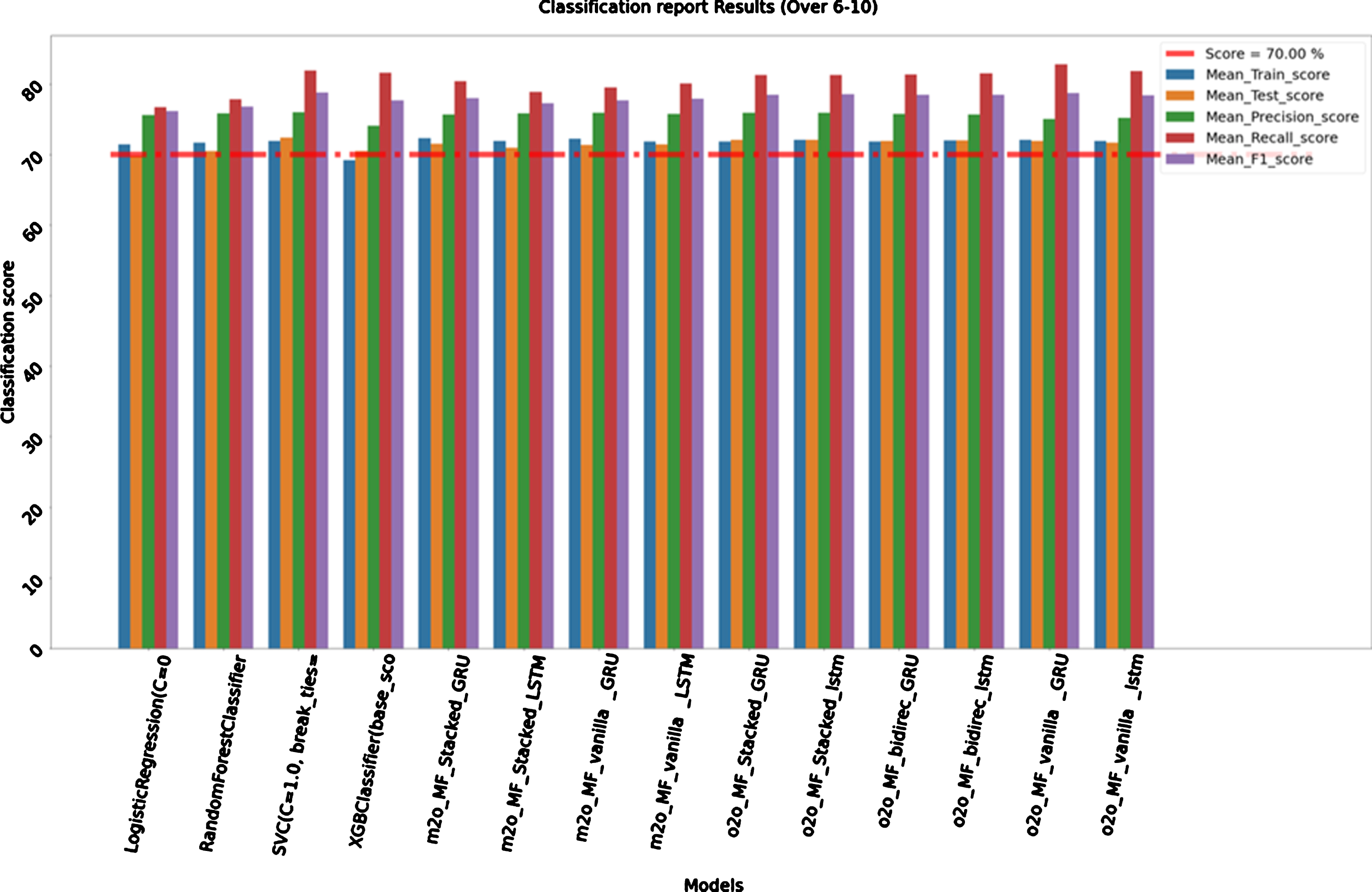
4.3MODEL 3 (6–10 over)
For this model we considered all records from 1 to 10 over of all seasons (2008–2018) to train our model and all 6 to 10 over of seasons (2019) to test it. Train size is 42,793 and test size is 1,820. Here also, again SVC from traditional machine learning and one-to-one sequence stacked LSTM from deep learning models shows good results during the next 5 overs of second inning. Table 5 results are from next 6 to 10 overs of the second inning. The train accuracies are 71.87%, and 72.06%with confidence interval of 2.07%, and 2.73%and test accuracies of 72.36%, and 72.09%respectively. One-to-one sequence vanilla GRU is showing exceptionally high Recall score of 82.75%. Again below is the comparative bar graph (Fig. 6) of results to have better visualization of performance of each algorithm between 6–10 overs.
Table 5
Classification Report Results (Over 6–10)
| Name | Mean_Train_score | Test_score | Precision_score | Recall_score | F1_score |
| Logistic Regression | 71.44%(+/–3.15%) | 69.84% | 75.58% | 76.71% | 76.14% |
| RandomForestClassifier | 71.69%(+/–3.16%) | 70.49% | 75.79% | 77.85% | 76.80% |
| SVC | 71.87%(+/–2.07%) | 72.36% | 75.95% | 81.87% | 78.80% |
| XGBClassifier | 69.17%(+/–3.65%) | 70.49% | 74.03% | 81.61% | 77.63% |
| m2o_MF_Stacked_GRU | 72.28%(+/–2.76%) | 71.51% | 75.70% | 80.35% | 77.96% |
| m2o_MF_Stacked_LSTM | 71.87%(+/–3.45%) | 70.96% | 75.80% | 78.86% | 77.30% |
| m2o_MF_vanilla_GRU | 72.24%(+/–2.48%) | 71.34% | 75.94% | 79.47% | 77.67% |
| m2o_MF_vanilla_LSTM | 71.86%(+/–2.69%) | 71.45% | 75.77% | 80.09% | 77.87% |
| o2o_MF_Stacked_GRU | 71.84%(+/–2.82%) | 72.03% | 75.88% | 81.26% | 78.48% |
| o2o_MF_Stacked_lstm | 72.06%(+/–2.73%) | 72.09% | 75.94% | 81.26% | 78.51% |
| o2o_MF_bidirec_GRU | 71.82%(+/–2.04%) | 71.92% | 75.71% | 81.35% | 78.43% |
| o2o_MF_bidirec_lstm | 71.98%(+/–2.66%) | 71.98% | 75.69% | 81.52% | 78.50% |
| o2o_MF_vanilla_GRU | 72.09%(+/–2.38%) | 71.87% | 75.00% | 82.75% | 78.68% |
| o2o_MF_vanilla_lstm | 71.88%(+/–2.46%) | 71.65% | 75.20% | 81.79% | 78.36% |
Fig. 6
Graph Classification Report Results (Over 6–10).
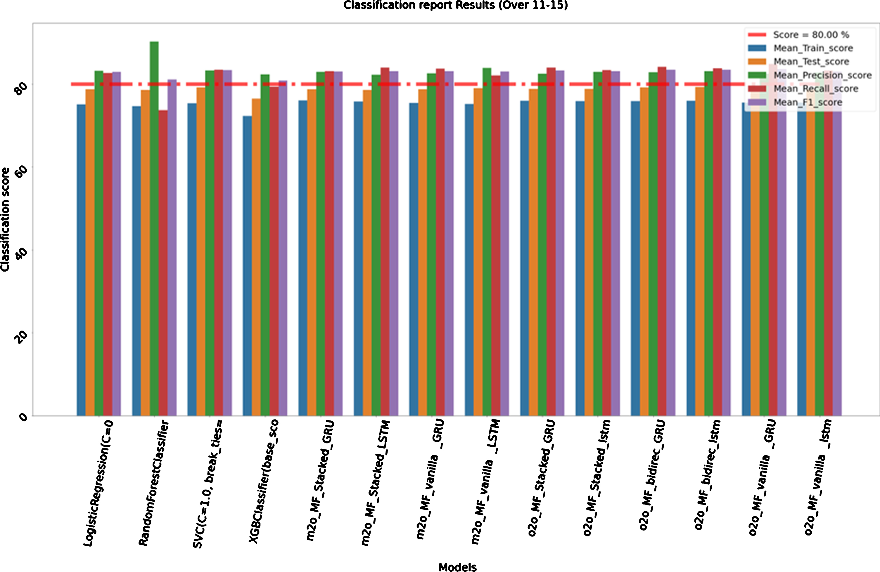
4.4MODEL 4 (11–15 over)
For this model we considered all records from 1 to 15 over of all seasons (2008–2018) to train our model and all 11 to 15 over of seasons (2019) to test it. Train size is 63,007 and test size is 1,829. Here as we can see deep learning models are showing best test scores as compared to traditional machine learning models. Table 6 results are from next 11 to 16 overs of the second inning. One-to-one sequence vanilla GRU and One-to-one Sequence Bidirectional LSTM are showing train accuracies of 76.02%and 75.58%with confidence interval of 3.50%, and 3.41%respectively. They are also showing good Precision, Recall and F1 scores near around 82.00%. As we can also see RandomForestClassifier is giving us a very good precision score of 90.26%on the test data. Again below (Fig. 7) is the comparative bar graph of above results to have better visualization of performance of each algorithm between 11–15 overs.
Table 6
Classification Report Results (Over 11–15)
| Name | Mean_Train_score | Test_score | Precision_score | Recall_score | F1_score |
| Logistic Regression | 75.15%(+/–3.94%) | 78.79% | 83.27% | 82.69% | 82.98% |
| RandomForestClassifier | 74.70%(+/–4.02%) | 78.57% | 90.26% | 73.69% | 81.14% |
| SVC | 75.39%(+/–3.43%) | 79.22% | 83.33% | 83.48% | 83.41% |
| XGBClassifier | 72.35%(+/–4.79%) | 76.49% | 82.40% | 79.37% | 80.85% |
| m2o_MF_Stacked_GRU | 76.10%(+/–3.74%) | 78.76% | 82.95% | 83.10% | 83.03% |
| m2o_MF_Stacked_LSTM | 75.78%(+/–3.55%) | 78.65% | 82.25% | 83.98% | 83.10% |
| m2o_MF_vanilla_GRU | 75.48%(+/–3.53%) | 78.82% | 82.63% | 83.71% | 83.17% |
| m2o_MF_vanilla_LSTM | 75.25%(+/–3.92%) | 79.04% | 83.97% | 82.14% | 83.05% |
| o2o_MF_Stacked_GRU | 76.00%(+/–3.45%) | 78.90% | 82.56% | 84.00% | 83.28% |
| o2o_MF_Stacked_lstm | 75.94%(+/–3.49%) | 78.90% | 82.96% | 83.39% | 83.17% |
| o2o_MF_bidirec_GRU | 75.90%(+/–3.42%) | 79.22% | 82.87% | 84.18% | 83.52% |
| o2o_MF_bidirec_lstm | 76.02%(+/–3.50%) | 79.28% | 83.17% | 83.83% | 83.50% |
| o2o_MF_vanilla_GRU | 75.58%(+/–3.41%) | 79.28% | 82.50% | 84.88% | 83.67% |
| o2o_MF_vanilla_lstm | 75.57%(+/–3.51%) | 78.73% | 82.80% | 83.30% | 83.05% |
Fig. 7
Graph Classification Report Results (Over 11–15).
4.5MODEL 5 (16–20 over)
For this model we considered all records from 1 to 20 over of all seasons (2008–2018) to train our model and all 16 to 20 over of seasons (2019) to test it. Train size is 79,129 and test size is 1,491. Logistic Regression shows accuracy of 76.48%(+/–2.94) during the last part of the match which is good. SVC and one-to-one sequence of bidirectional GRU also gives accuracies close to 76.00%. They are giving test score of 77.26%and 77.13%respectively as we are close to end of the second inning. We can see that almost all models are showing a very good Recall
score of close to 100.00%which is very good as it shows in low false negative rate. So our model had ability to find all the relevant cases within the dataset. While recall expresses the ability to find all relevant instances in a dataset, precision expresses the proportion of the data points our model says was relevant actually were relevant. Below is the comparative bar graph (Fig. 8) of above results to have better visualization of performance of each algorithm between 16–20 overs.
Fig. 8
Graph Classification Report Results (Over 16–20).
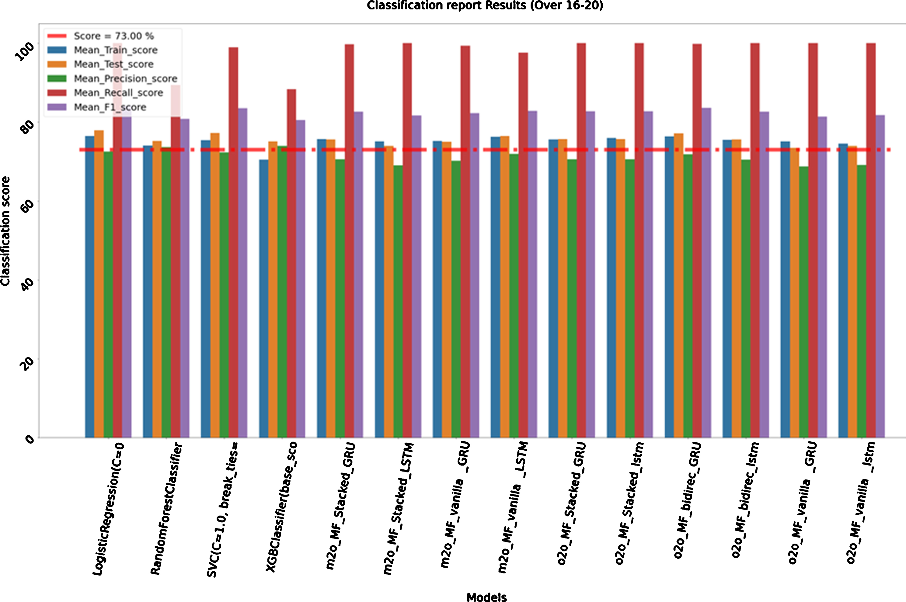
Table 7
Classification Report Results (Over 16–20)
| Name | Mean_Train_score | Test_score | Precision_score | Recall_score | F1_score |
| Logistic Regression | 76.48%(+/–2.94%) | 77.93% | 72.54% | 100.00% | 84.08% |
| RandomForestClassifier | 74.01%(+/–3.59%) | 75.18% | 73.65% | 89.41% | 80.77% |
| SVC | 75.38%(+/–2.85%) | 77.26% | 72.27% | 98.96% | 83.54% |
| XGBClassifier | 70.46%(+/–4.21%) | 75.12% | 73.99% | 88.38% | 80.55% |
| m2o_MF_Stacked_GRU | 75.65%(+/–2.71%) | 75.62% | 70.55% | 99.77% | 82.66% |
| m2o_MF_Stacked_LSTM | 75.10%(+/–3.54%) | 73.94% | 69.08% | 100.00% | 81.72% |
| m2o_MF_vanilla_GRU | 75.24%(+/–2.82%) | 75.02% | 70.17% | 99.31% | 82.23% |
| m2o_MF_vanilla_LSTM | 76.32%(+/–3.19%) | 76.43% | 71.94% | 97.58% | 82.82% |
| o2o_MF_Stacked_GRU | 75.57%(+/–3.11%) | 75.65% | 70.54% | 100.00% | 82.72% |
| o2o_MF_Stacked_lstm | 76.02%(+/–2.69%) | 75.72% | 70.59% | 100.00% | 82.76% |
| o2o_MF_bidirec_GRU | 76.33%(+/–2.54%) | 77.13% | 71.85% | 99.88% | 83.58% |
| o2o_MF_bidirec_lstm | 75.51%(+/–3.32%) | 75.59% | 70.48% | 100.00% | 82.68% |
| o2o_MF_vanilla_GRU | 75.12%(+/–3.58%) | 73.44% | 68.70% | 100.00% | 81.44% |
| o2o_MF_vanilla_lstm | 74.58%(+/–3.49%) | 73.98% | 69.13% | 100.00% | 81.75% |
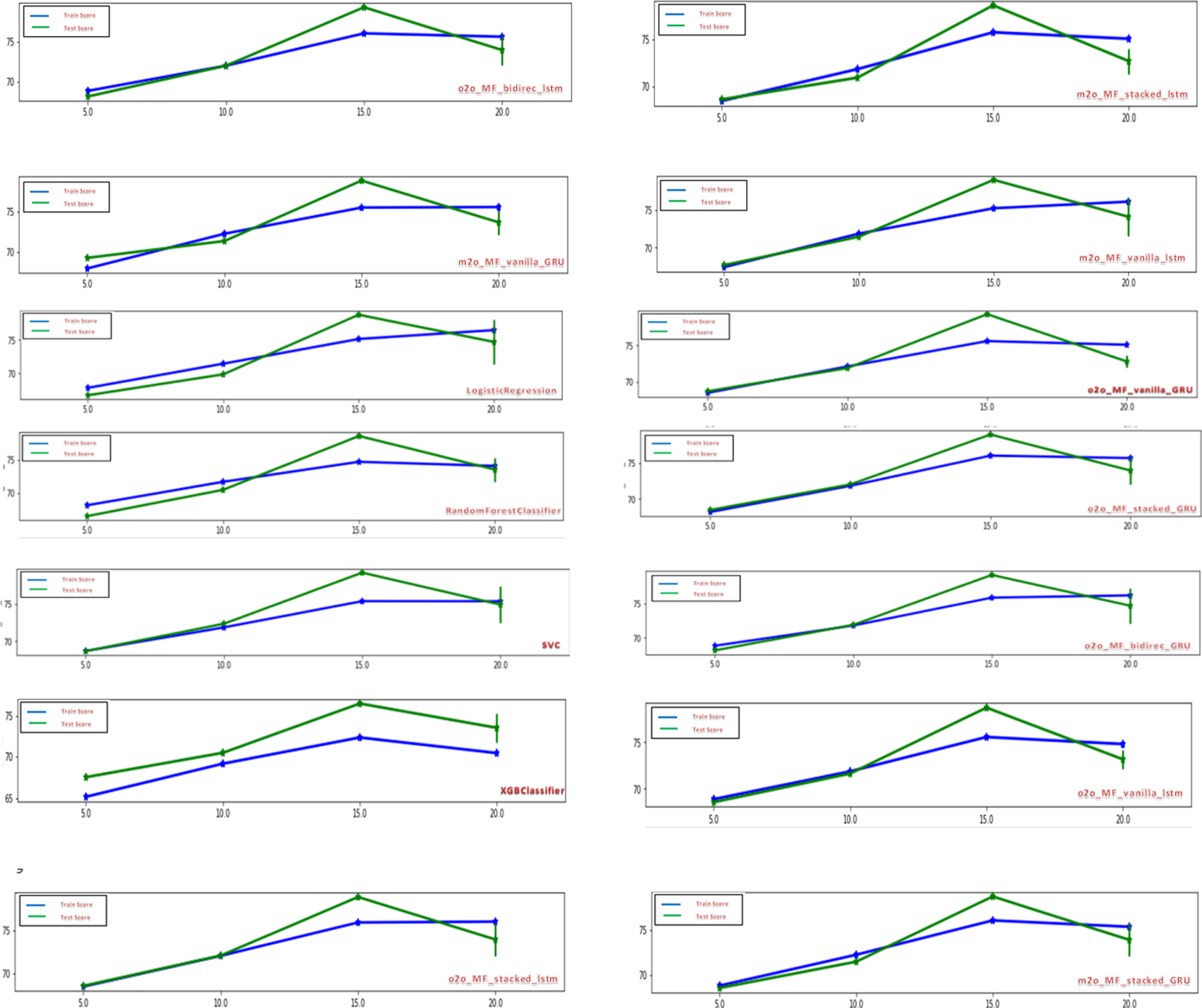
Below (Fig. 9) is the comparative trend graph of train and test scores for all the traditional and deep learning models during the second inning of the match. The blue line shows the train score and the green line shows the test score across various intervals of overs. One thing we can observe across the models is that almost all the models give very good prediction during the start of 15th over. Test scores are higher than train scores. But still there are few models like SVC, XGBClassifier, and one-to-one stacked GRU which gives good test scores as compared to their train score from start of the second inning itself.
Fig. 9
Trend chart of Train and Test scores during the second inning.
5Conclusion and future work
For this paper we considered 692 matches of all the seasons (2008–2018) to train our model and all the 59 matches of season (2019) to test. In future we can start right from the beginning of the first inning. Although our study is done on IPL Twenty20 matches only, the however similar approach could be applied to predict outcome in other versions of Cricket matches as well i.e. test cricket and ODI matches. We can apply these Classification techniques to other sports such as football, tennis, although the method of implementation might differ from one sport to another. We also planned to handle the results of the matches which are interrupted by rainfall or other natural calamities. So for that we would need to work on how to handle such scenarios with the help of Duckworth-Lewis method. Winning or losing a match greatly depends on selection of right players for each match. An accurate prediction of how many runs a batsman is likely to score and how many wickets a bowler is likely to take in a match will help the team management select best players for each match. The Twenty20 format of cricket carries a lot of randomness, because a single over can completely change the ongoing pace of the game. Indian Premier League is still at infantry stage; it is just a decade old league and has way less number of matches compared to test and one-day international formats. The IPL is the most popularly viewed game in the world. In 2019 the brand value of the IPL was estimated to be 475 billion (US$6.7 billion), according to Duff & Phelps. According to BCCI, the 2015 IPL season contributed 11.5 billion (US$160 million) to the GDP of the Indian economy. According to BCCI, the 2015 IPL season contributed 11.5 billion (US$160 million) to the GDP of the Indian economy. Given the scale of the betting industry worldwide, there are obviously monetary gains for anyone with access to superior prediction techniques, whether through working with betting companies, selling predictions to professional gamblers or personal betting. This study can benefit cricket club managers, sport data analysts and scholars interested in sport analytics, among others.
References
1 | Lamsal, R. and Choudhary, A. , 2018, Predicting outcome of Indian Premier League (IPL) matches using machine learning, arXiv [stat.AP]. |
2 | Sankaranarayanan, V.V. , Sattar, J. and Lakshmanan, L.V.S. , (2014) , Auto-play: A data mining approach to ODI cricket simulation and prediction, in Proceedings of the 2014 SIAM International Conference on Data Mining, Philadelphia, PA: Society for Industrial and Applied Mathematics, pp. 1064–1072. |
3 | Jayanth, S.B. , Anthony, A. , Abhilasha, G. , Shaik, N. and Srinivasa, G. , (2018) , A team recommendation system and outcome prediction for the game of cricket, J Sports Anal, 4: ((4)), 263–227. |
4 | Pathak, N. and Wadhwa, H. , (2016) , Applications of modern classification techniques to predict the outcome of ODI cricket, Procedia Comput Sci, 87: , pp. 55–60. |
5 | Bhattacharjee, D. and Talukdar, P. , 2019, Predicting outcome of matches using pressure index: evidence from Twenty cricket, Commun Stat Simul Comput, pp. 1–13. |
6 | Deep, C. , Patvardhan, C. and Vasantha, C. , (2016) ,Data analytics based deep mayo predictor for IPL-9, Int J Comput Appl, 152: ((6)), 6–11. |
7 | (2019) , Forecasting the outcome of the next ODI cricket matches to be played, Regular Issue, 8: ((4)), 10269–10273. |
8 | Manivannan, S. and Kausik, M. , (2019) , Convolutional neural network and feature encoding for predicting the outcome of cricket matches, in 2019 14th Conference on Industrial and Information Systems (ICIIS). |
9 | Passi, K. and Pandey, N. , 2018, Increased prediction accuracy in the game of cricket using machine learning, arXiv [cs.OH]. |
10 | Singh, S. and Kaur, P. , (2017) , IPL visualization and prediction using HBase, Procedia Comput Sci, 122: , 910–915. |
11 | Passi, K. and Pandey, N. , (2018) , Predicting players’ performance in one day international cricket matches using machine learning, in Computer Science & Information Technology. |
12 | Bailey, M. and Clarke, S.R. , (2006) , Predicting the match outcome in one day international cricket matches, while the game is in progress, J Sports Sci Med, 5: ((4)), 480–48. |
13 | Ul Mustafa, R. , Nawaz, M.S. , Ullah Lali, M.I. , Zia, T. and Mehmood, W. , (2017) ,Predicting the cricket match outcome using crowd opinions on social networks: A comparative study of machine learning methods, Malays J Comput Sci, 30: ((1)), 63–76. |
14 | Percy, D.F. , (2015) , Strategy selection and outcome prediction in sport using dynamic learning for stochastic processes, J Oper Res Soc, 66: ((11)), 1840–1849. |
15 | Kampakis, S. and Thomas, W. , 2015,Using machine learning to predict the outcome of English county twenty over cricket matches, arXiv [stat.ML]. |
16 | Singh, T. , Singla, V. and Bhatia, P. , (2015) , Score and winning prediction in cricket through data mining, in 2015 International Conference on Soft Computing Techniques and Implementations (ICSCTI). |
17 | Tandon, N. , Varde, A.S. and de Melo, G. , (2018) , Commonsense knowledge in machine intelligence, SIGMOD Rec, 46: ((4)), 49–52. |
18 | Van den Berg, L. , Coetzee, B. , Blignaut, S. and Mearns, M. , (2018) , The competitive intelligence process in sport: data collection properties of high-level cricket coaches, Int J Perform Anal Sport, 18: ((1)), 32–54. |
19 | De Melo, , Gerard and Varde, Aparna, , 2015, Scalable Learning Technologies for Big Data Mining. |
20 | Schoeman, J.H. , Matthee, M.C. , Van der Merwe, P. , (2006) , The viability of business data mining in the sports environment: cricket match analysis as application, S.A. j. res. sport phys. educ. recreat, 28: ((1)). |
21 | Basavaraju, P. and Varde, A.S. , (2017) , Supervised learning techniques in mobile device apps for androids, SIGKDD Explor, 18: ((2)), 18–29. |
22 | Maheswari, P.U. , A Novel Approach for Mining Association Rules on Sports Data using Principal. |
23 | Kaluarachchi, A. and Aparna, S.V. , (2010) , CricAI: A classification based tool to predict the outcome in ODI cricket, 2010 Fifth International Conference on Information and Automation for Sustainability, pp. 250–255. |


