
Conditional probability and the length of a championship series in baseball, basketball, and hockey
Abstract
This paper re-examines the assumption that the probability of winning the World Series, the NBA Finals, and the Stanley Cup is constant across the series. This assumption is the primary basis for models that endeavor to explain the length of a series, but we demonstrate that this model is inconsistent with historical data in all three sports. We adjust the model to incorporate conditional probabilities and fit it with historical data. While one can always backfit historical frequencies to conditional probabilities, doing so shows that the variation in conditional frequencies within and across sports is too wide to support the constant probability model. We also define a new notion of the concept of two teams being evenly matched.
Sports championships draw considerable interest from the general public, the media, and statisticians. Major League Baseball’s World Series, the National Basketball Association’s Finals, and the National Hockey League’s Stanley Cup are all best-of-seven series that are watched and followed by millions of people worldwide. Fans wait with great anticipation for the outcomes of these events, not knowing if a series will go four, five, six, or seven games. Broadcasters pay millions of dollars for the rights to televise these games, thereby making substantial investments in an event with uncertain length. Moreover, a considerable amount of money is wagered on these games, some legal and a great deal illegal.
An obvious question that arises from these best-of-seven events is the number of games required to determine the winner. Only a modest amount of research, however, and amounting to but four scientific studies, has been done on this subject. All of these studies have been based on the assumption that the games represent a series of independent events with each team having a constant probability of winning a given game. Naturally, the naïve assumption is that this probability is 0.5, a condition often referred to as the teams being “evenly matched.” Perhaps this assumption is simply convenient, though perhaps it is motivated by the fact that the series is between the two best playing teams at the time, and thus, they are likely to be similar in quality. As we discuss later, an argument can be made that an evenly-matched series is not the same notion as an evenly-matched game. Nonetheless, this issue can be set aside for the moment. The primary question of this paper is whether the probability of victory is constant throughout the series and if not, how we can incorporate a non-constant probability of a given team winning. In previous analyses, a model based on constant probability and independence has always been assumed, and some researchers have attempted to extract that probability from the data.
In this paper, we present evidence that these assumptions are incorrect and lead to results that are inconsistent with the history of these sports championships. We develop an improved model for the distribution of games by incorporating conditional probability, the notion that a team is more or less likely to win based on certain conditions that exist at a given time. While one can always fit conditional probabilities to historical data, in doing so we show that the variation across and within sports is too great to support the constant probability model. In particular, a constant probability of 0.5 is a poor fit.
1Previous research
Only a few studies addressing the issue of the distribution of games have appeared in the scholarly literature. Mosteller (1952) examines the question of whether a seven-game World Series is sufficient for identifying the so-called “better” team. He derives a maximum likelihood estimates of a constant probability of one team winning each game of
Groeneveld and Meeden (1975) examine data from the World Series (1903–1973), NBA (1950–1973), and National Hockey League (1939–1967) with the objective of obtaining a single best probability estimate. They obtain maximum likelihood estimates of a constant probability of
Using World Series data from 1903–2005, Cassuto and Lowenthal (2007, 2011) examine the issue from an economic perspective. They argue that those with an economic interest in the event should be concerned about the likelihood of the event lasting four, five, six, or seven games. Their examination is couched in the following manner. Consider the multinomial X = (X4, X5, X6, X7) where Xi is the number of games the series lasts, i = 4, ... 7. Cassuto and Lowenthal use the chi-square test with three degrees of freedom to examine the null hypothesis that
The constant probability model has also been in used in other studies directed at related but different sports issues. For example, Ben-Naim et al. (2012) employ a constant probability model to examine the efficacy of single-elimination tournaments in contrast to each team playing each other team. The blogosphere has also contained discussion about the probabilities of the number of games.3 Although several of these previous papers and discussions raise the issue that the probabilities may not be constant, all generally work with the independent constant probability assumption or leave the matter for others to resolve. In short, the research on this question has not proposed, what more examined, an alternative to the model of constant probability and independence.
In an excellent treatment of the mathematics of baseball, Ross (2007) shows how the ex ante distribution of games is determined, and he acknowledges that a probability of 0.5 does not fit the data very well. He states, however, that it is difficult to determine any other probability. He discusses the possibility of a conditional probability model but only in the context of a model in which one team is the favorite. For example, a favorite would be defined as a team having a probability of winning a game of more than 0.5. He then examines the formulas for the probability of a series lasting a certain number of games given that the favorite has already won or lost some games. Our work extends the idea of conditional probability by using historical data, but in our model any so-called favorite, could, for example, be the favorite after one or two games and the underdog later. We let the historical data tell us when these probabilities change.
In this study, we formalize the application of conditional probability to the model of seven-game championship series and thereby fill a much needed space in the evolution of formal models of these events.4
2Specification of the problem
If we begin with the assumption that an arbitrary team, say team A, has a probability p of winning each game, it is a simple matter to determine the probability that a series will last four, five, six, or seven games.5 Denoting those probabilities as Pr(i), the probability that a series will last i games where i = 4, 5, 6, or 7, we have
The general formula is
Under the naïve assumption that p = 0.5, Table 1 shows these probabilities. They are, of course, well-known and documented in the literature. The expected number of games is as follows:
Table 1
The Probabilities that a Best-of-Seven Series goes Four, Five, Six, or Seven Games (Pr(i), i = 4, 5, 6, 7) under the assumption that each team has a 50% probability of winning each game
| Number of Games (i) | Pr(i) |
| 4 | 12.50% |
| 5 | 25.00% |
| 6 | 31.25% |
| 7 | 31.25% |
| 100.00% |
As we will show, however, these probabilities and hence the constant probability assumption is a poor match to the observed relative frequencies, especially for certain sports.
3The data
We collect data for baseball’s World Series, basketball’s NBA Finals, and hockey’s Stanley Cup finals, the latter hereafter referred to simply as the “Stanley Cup.” The World Series began in 1903 but followed an inconsistent format until 1923. In some cases the Series was based on a best-of-seven structure, in others a best-of-nine structure, and in some years, tied games were permitted. Since 1923 however, the series has been played with a consistent best-of-seven format with tied games extending into extra innings until a winner is determined. Thus, we collect data starting in 1923 through 2018 from www.baseballreference.com. There are 551 World Series games played during that period.
The National Basketball Association was founded in 1949 as a successor to the Basketball Association of America. Its 1949–1950 season was played with 15 teams divided into three divisions. From the 1950–1951 season forward, it has been divided into Eastern and Western Divisions, which in some years are called “Conferences,” and in later years further broken into sub-divisions. We start with this second season of the NBA’s history, 1950–1951, and collect data through the 2017–2018 season from www.basketballreference.com.6 There are 392 games played in the Championship finals during that period.
The National Hockey League was founded in 1917, and the league structure has changed many times. Not until 1968 did the league divide itself into eastern and western divisions. In 1975 it then realigned into the Clarence Campbell and Prince of Wales Conferences, each with three divisions. Nonetheless, these divisions did not compete with each other in the playoffs until 1982. In other words, until 1982, two teams from the same conference could end up competing in the finals for the Stanley Cup. In 1994 the structure was changed again, this time into eastern and western conferences, whereby the Stanley Cup finals would match the playoff champions of the eastern and western conference. For the hockey data, we start with 1939, because that was the first year the Stanley Cup followed a best-of-seven format that it has retained since that time. The data sources are www.hockey-reference.com and www.nhl.com and go through the 2017-2018 season. After accounting for the cancelation of the 2005 NHL season, there are 403 Stanley Cup finals games played during that period.
Table 2 provides descriptive statistics of the 95 World Series, 68 NBA Finals, and 79 Stanley Cup Finals in the data set. Although not shown in the table, a total of 36 teams have appeared in the World Series, 30 in the NBA Finals, and 28 in the Stanley Cup Finals.7 Of course, the New York Yankees have been a dominant team in baseball, appearing in 38 series, winning 27. The second most successful team has been the St. Louis Cardinals, who have appeared in 19 series, winning 11. The Pittsburgh Pirates have won four of five series, for the best winning percentage with four or more series. The most unsuccessful team that has competed in at least one series would be the Brooklyn Dodgers who appeared in seven series, winning only one (1955).
Table 2
Descriptive Statistics of the World Series and NBA Finals
| World Series (1923–2018) | NBA Finals (1951–2018) | Stanley Cup (1939–2018) | |
| Number of Series | 95 | 68 | 79 |
| Team with most appearances | New York Yankees (38) | Los Angeles Lakers (25) | Montreal Canadians (27) |
| Team with most championship wins | New York Yankees (27) | Boston Celtics (17) | Montreal Canadians (20) |
| Team with most championship losses | New York Yankees (11) | Los Angeles Lakers (14) | Detroit Red Wings (12) |
| Team with highest winning pct., four or more series | Pittsburgh Pirates | Chicago Bulls | Pittsburgh Penguins |
| (80%, 5 series) | (100%, 6 series) | (83.33%, 6 series) | |
| Team with lowest winning pct., four or more series | Chicago Cubs | Cleveland Cavaliers | Philadelphia Flyers |
| (16.67% 6 series) | (20%, 5 series) | (25%, 8 series) | |
| Home team wins game | 56.20% | 61.73% | 60.56% |
| Team with most home games in series wins series* | 45.61% | 66.67% | 75.68% |
| Team with better season record wins series | 51.09% | 73.44% | 77.46% |
| Travel Formats | |||
| 1-1-1-1-1-1-1 | 1 | 2 | 1 |
| 2-3-2 | 91 | 31 | 2 |
| 3-4 | 3 | 0 | 0 |
| 2-2-1-1-1 | 0 | 33 | 74 |
| 1-2-2-1-1 | 0 | 2 | 0 |
| 1-2-4 | 0 | 0 | 1 |
| Indeterminate** | 0 | 0 | 1 |
Note: The data used here do not constitute the entire history of many teams. For series not lasting seven games, travel formats are estimates based on patterns to that point and patterns used in nearby years. Performance is counted separately by team/city and not by franchise. *The team with most home games refers to the team with most home games played in the series, not the team with the most home games scheduled. **The indeterminate Stanley Cup series was in 1940 in which the first two games were played in New York, and the next four were played in Toronto, with the series ending in six games. The pattern of 2-4, which occurred because of a circus booked in Madison Square Garden, is not observed anywhere else in the hockey, baseball, or basketball data. It is difficult to estimate for certain where the seventh game would have been played. It probably would have gone back to New York for a 2-4-1 pattern, which is unusual and not observed anywhere else, or due to the circus, it may have been forced to remain in Toronto for a 2-5 pattern, which is also unusual and did not occur anywhere else.
The NBA has been dominated by the Boston Celtics and Los Angeles Lakers. The Celtics have appeared in 21 Finals, winning 17. The Los Angeles Lakers have appeared in 25 Finals, winning 11, and the Laker franchise also appeared in four other finals, winning three, as the Minneapolis Lakers. Two other very successful franchises are the Chicago Bulls, who have won all six of their appearances, and the San Antonio Spurs, who have won five of six. The worst record for a team that has appeared at least four times is the Cleveland Cavaliers who have won one of five series.
The most successful hockey teams have been the Montreal Canadians, Detroit Red Wings, Boston Bruins, and Toronto Maple Leafs. Montreal has won 20 of 27 Stanley Cup finals, while Detroit has won 9 and lost 12, and Boston has won five and lost 11. The Toronto Maple Leafs have appeared 14 times, winning 10, and the Chicago Black Hawks have won four and lost six. Of course, these are the oldest teams in the league, and thus, they have had more opportunities and less competition.
The table also shows some data on the home-away record. The home advantage can be interpreted several ways. One is the obvious notion of a home advantage for a given game. The team at home has won 56.20% of World Series games, 61.73% of NBA Finals games, and 60.56% of Stanley Cup Finals games. An alternative notion of home advantage is that the team that plays more home games in the series has an advantage. Under this definition of home advantage, the team with the edge has won 45.61% of World Series championships, 66.67% of NBA Championships, and 75.68% of Stanley Cups.8
Of the two competing teams, the one with the better season record has won 50.57% of World Series, 72.88% of NBA Championships, and 77.46% of Stanley Cups. These results shed some light on whether many of these series have been mismatched, meaning that there is simply a stronger team. That could be the case in hockey as well as basketball, but it does not appear to be the case in baseball.
The last section of the table shows the various home-away formats used by the leagues. Baseball has followed the 2-3-2 format for 91 of 95 series, with two games in one city, the next three in the other city, and the final two in the first city. Basketball has used four different formats with 31 following the 2-3-2 format and 33 following the 2-2-1-1-1 format in which the last three games alternate cities. Hockey has used the 2-2-1-1-1 format for 74 of 79 series.9
4Comparison of the Data with the p = 0.5 Model
Table 3 shows the observed frequencies of four-, five-, six-, and seven-game series along with the expected frequencies under on the naïve assumption of a 0.5 probability for each game. As can be seen, there have been far more four- and seven-game World Series, and correspondingly fewer five- and six-game series that would be expected if in each game, each team had a 50% chance of winning. The average number of games, however, at 5.80 is almost precisely equal to the expected number of 5.81. This finding immediately makes us believe that 0.5 is the appropriate parameter. But, we have fit only the mean of the distribution. The assumption of a 0.5 probability is not very accurate, as indicated by the fact that the chi-square goodness of fit statistic,
Table 3
Observed Relative and Expected Frequencies of Four-, Five-, Six-, and Seven-Game Series in the World Series, NBA Finals, and Stanley Cup
| Series ends in i games | World Series | NBA Finals | Stanley Cup | Expected Frequencies of Games (p = 0.5) |
| Observed Frequencies | ||||
| 4 | 18.95% | 13.24% | 25.32% | 12.50% |
| 5 | 21.05% | 25.00% | 22.78% | 25.00% |
| 6 | 21.05% | 33.82% | 31.65% | 31.25% |
| 7 | 38.95% | 27.94% | 20.25% | 31.25% |
| Average # of games based on observed or expected frequencies | 5.80 | 5.76 | 5.47 | 5.81 |
| Chi-square (p-value) | 8.71 (0.0334) | 0.41 (0.0622) | 181.15 (0.0035) | _ |
Interestingly, the NBA data come much closer to fitting the p = 0.5 model. The number of five-game series is precisely the theoretical value and the other observed and expected frequencies are somewhat close to their theoretical values, and the average number of games, at 5.76, is close to the expected number of 5.81. Nonetheless, the null is still rejected with a Type I error of only 6.2%. In addition, as we will show later, it is possible to obtain a better fit for NBA data and plenty of reasons to prefer one.
For the Stanley Cup, the differences between the observed and the expected frequencies are quite high. The percentage of four-game series is more than twice the expected number. This disproportionate result comes mostly at the expense of seven-game series, with about 20% of Stanley Cup finals going to seven games, while the expected percentage is slightly more than 31%. The average observed number of games of 5.47 is notably lower than the expected number under the 0.5 hypothesis, and the chi-square test rejects the null hypothesis at better than the 1% level. Thus, the evidence suggests that a model with a constant probability of 0.5 does not fit hockey or baseball at all and probably not even basketball.
5Alternative Estimates of p
We may be able to salvage the constant probability model if we can find a probability other than 0.5 that fits the data reasonably well. Consider first the World Series, in which we have too many seven-game series in relation to the number we would expect if p = 0.5. We first might wonder if we can alter the constant probability model to better fit the data, but we show in Appendix A that if a constant probability is assumed, the probability of a seven-game series is maximized at p = 0.5. Since the observed number of seven-game series is more than the expected number at p = 0.5, any other value of p will certainly take the expected number of seven-game series even further away from the observed number.
In spite of this impossibility, Mosteller (1952) suggests two ways of fitting a single probability estimate to the data. First, he suggests matching the expected value with the average number of games played.10 We do this for the World Series and obtain
For the NBA Finals, we obtain
Mosteller also suggests a maximum likelihood approach to identifying a single constant probability. In other words, given the observed data, which probability maximizes the likelihood that the sample would have occurred? Following Mosteller’s approach, let pL (j) = the probability that the team that loses the series wins j games, where j = 0, 1, 2, or 3. The multinomial probability of drawing the sample is
Fig. 1
Maximum Likelihood Estimate of Constant Probability of One Team Winning the World Series, NBA Finals, and Stanley Cup. A. World Series. B. NBA Finals. C. Stanley Cup. The line is the value pL (0) N(4)pL (1) N(5)pL (2) N(6)pL (3) N(7), ,which is the kernel of the multinomial likelihood function where pL (j) is the probability that the team that loses the series wins j games (j = 0, 1, 2, or 3) and N(i) is the number of four-, five-, six-, and seven-game series that have occurred. The observed maxima identify the maximum likelihood estimates of a constant probability of one team winning.
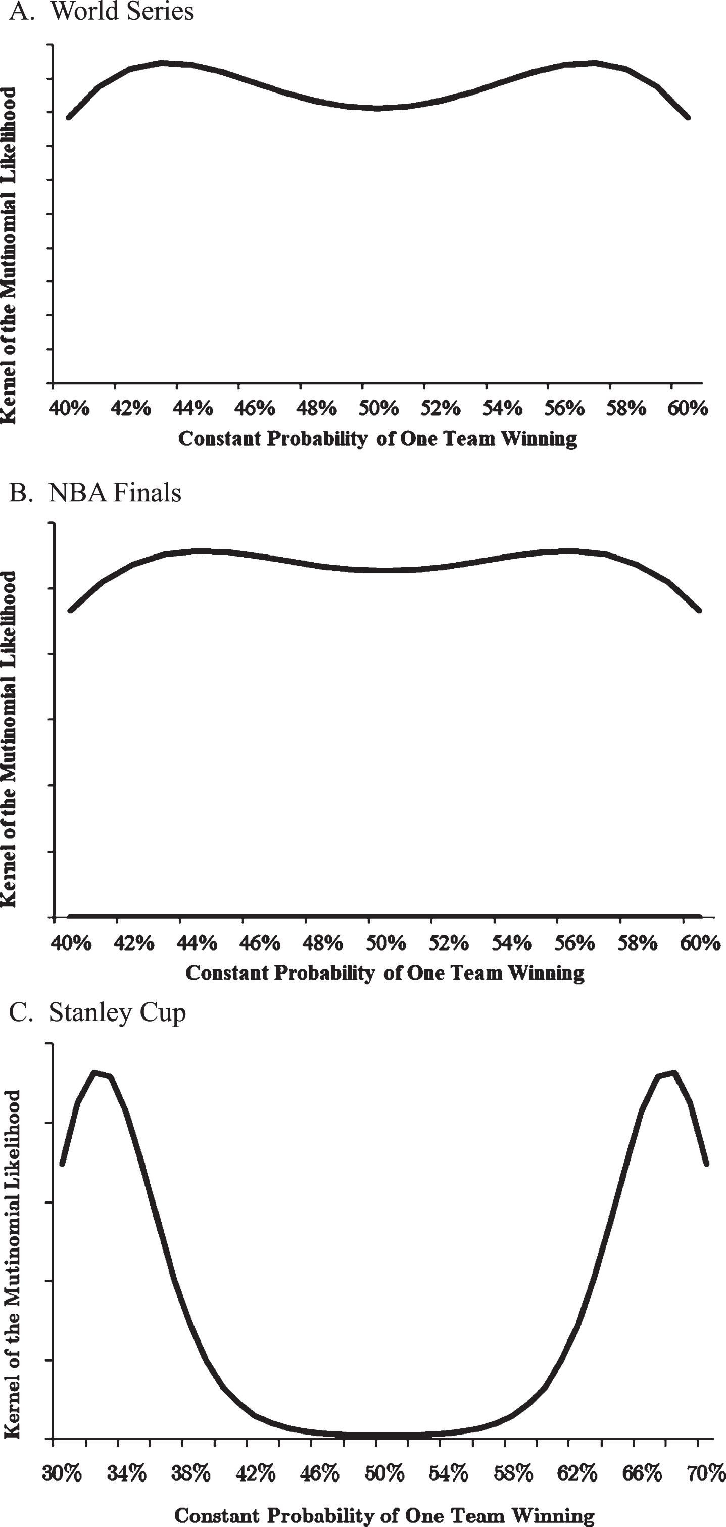
For baseball, Fig. 1A, we see that the probability of observing 18 four-game series, 20 five-game series, 20 six-game series, and 37 seven-game series is maximized at roughly
In Fig. 1B, for the NBA, we find yet another disconcerting result. While the maximum occurs at
For the Stanley Cup, Fig. 1C, we have maxima at around
Hence, for baseball, no single value of p seems appropriate. For basketball multiple values of p seem to fit the data. For hockey, extreme values of p best fit the data.
6A Model using conditional probability
In this section we attempt to determine if we can improve the model of the number of games in best-of-seven championship series by incorporating conditional probability. Historical data can be tabulated based on conditions that exist to that point to provide estimates of conditional probabilities. Naturally we can always fit a model to historical conditional frequencies. The insight of this analysis is to reveal the extent to which the conditional probabilities vary across different conditions. If they do not vary much, then a conditional probability model will not be an improvement over a constant probability model.
Table 4 takes this approach by showing the relative frequencies with which teams win, given their previous wins in the series. The corresponding numbers in parentheses are the numbers of occurrences of the condition. Thus, for example, in the second line for the World Series one team has been ahead two games-to-none 46 times, and it has won the third game 43.48% of the time.
Table 4
Relative Frequencies of Various Conditioning Events in the World Series and NBA Finals
| Condition | World Series | NBA Finals | Stanley Cup |
| Team ahead 1-game-to-0 wins game 2 | 48.42% (95) | 47.06% (68) | 64.56% (79) |
| Team ahead 2-games-to-0 wins game 3 | 43.48% (46) | 37.50% (32) | 52.94% (51) |
| Team ahead 2-games-to-1 wins game 4 | 46.67% (75) | 48.21% (56) | 51.92% (52) |
| Team ahead 3-games-to-0 wins game 4 | 90.00% (20) | 75.00% (12) | 74.07% (27) |
| Team ahead 3-games-to-1 wins game 5 | 54.05% (37) | 56.67% (60) | 55.88% (34) |
| Team ahead 3-games-to-2 wins game 6 | 35.09% (57) | 54.76% (42) | 60.00% (40) |
Note: The numbers in parentheses equal the number of possible events. Thus, in baseball, of the 95 times in which one team was ahead one-game-to-none, 46 (≈ 48.42% ×90) times, the team won and went ahead two-games-to-none. In the remaining 49 times, the team behind won and tied the series at one game apiece.
In baseball, we see that the team winning the first game has won the second game a little less than 49% of the time, and when it wins the second game, it wins the third game about 47% of the time. Yet if it wins the third game, it wins the fourth game and sweeps the series 90% of the time. A team ahead two- games-to-one wins the fourth game about 47% of the time, while a team ahead three-games-to-one wins the fifth game about 54% of the time. Perhaps most strikingly, a team ahead three-games-to-two wins the sixth game only about 35% of the time. In other words, the team with its back to the wall, down three games-to-two, wins almost two-thirds of the time to send the series into the seventh game. This phenomenon explains why the number of seven-game series is so large in relation to what is implied by the p = 0.5 model. We will explore this result in more detail later.
Turning to basketball, a team up one game-to-none wins the second game about 47% of the time. Being up two games-to-none, however, has been a much more difficult situation, with the team ahead winning only about 38% of the time. If the team is ahead two games-to-one, it wins game four about 48% of the time. As with baseball, a team ahead three games-to-none has a very high chance (75%) of a four-game sweep. Teams ahead three games-to-one and three games-to-two have won the next game about 57% and 55% of the time, respectively. In the latter case, with a team behind three games-to-two and winning the sixth game only about 45% of the time, we would expect a somewhat smaller number of seven-game series than would occur with the constant probability and independence model. And indeed, that is the case, as was shown in Table 3.
For the Stanley Cup, teams that win the first game go on to win the second game about 65% of the time. If a team is up two games-to-none, it wins the third game about 52% of the time. If it is up three-games-to-none it wins the fourth about 74% of the time.13
To summarize, if the constant probability and independence model were correct, these conditional frequencies would be approximately the same. Some modest variation might be expected and indeed a number of these frequencies are close to 50%. But too many are far away from 50%. From this data, we can easily see that baseball has too many seven-game series and too few six-game series because teams behind three-games-to-two tend to win at far better than a 50% rate. It also has too many four-game series because teams ahead three-games-to-none sweep the series 90% of the time. Basketball fits the constant probability rule more closely than the other two sports, but it has a bit too few seven-game series and slightly more six-game series because teams up three-games-to-two win the sixth game at well more than a 50% rate. Hockey has far too many four-game series because teams up three-games-to-none win and sweep 75% of the time. It has too few seven-game series, because teams ahead three-games-to-two win the sixth game 60% of the time. In addition, the excessive number of four-game sweeps also reduces the number of seven-game series. These results are completely inconsistent with the constant probability model.
In addition, by using historical data we can fit the distribution exactly, without having to know the odds of one team winning when the series is tied. In fact, the probabilities when the series is tied are irrelevant as there is no pre-condition that favors one team. Hence, we can assume p0,0 = p1,1 = p2,2 = p3,3 = 0.5 Letpk, m be the probability that a team will win the (k + m+1)th game, having previously won k games and lost m games. We first determine the probability that the series will last four games. The probability of an arbitrary team A winning the series in four games is
The series could also end in four games if team A loses the first four games. If the conditional probabilities apply equally to each team, then the probability of team A losing all four games is14
Thus, the probability that the series ends in four games is the sum of these probabilities,
Now consider the probability that the series will end in five games, Pr(5). By definition, Pr(5) is the probability that after four games, one team is up three-games-to-one and that team wins the fifth game.15 There are eight possible ways that teams A and B can play four games and have one team win three and the other win one. Denoting the series-winning team as either A or B, the eight possible sequences of winners are AAAB, AABA, BAAA, ABAA, BBBA, BBAB, ABBB, and BABB. For the series to end on the fifth game, we must append to these eight sequences either A or B such that A or B has four wins. For team A to win, the outcomes would have to be AAABA, AABAA, BAAAA, and ABAAA. For team B to win, the outcomes would be BBBAB, BBABB, ABBBB, and BABBB. Appendix B shows that the probabilities of these events combine to
(1)
Now consider the probability that the series ends in six games. Given what we already know, this result is easy to obtain. First consider that the probability that the series lasts at least six games is 1 –Pr(4) –Pr(5). The probability that the series lasts exactly six games is the probability that it lasts at least six games times the probability that the team ahead three-games-to-two wins the sixth game.16 Thus,
And finally, the probability that the series lasts seven games is simply the complement of the probabilities we have obtained to this point,
Using this information and estimates of the conditional probabilities from the historical frequencies, we can match the distribution of games precisely. The results are obtained by building a binomial tree for the 70 sequences, inserting the probabilities of each path, and doing the appropriate multiplications. Results are verified using the equations above for Pr(4), Pr(5), Pr(6), and Pr(7). Table 5 presents these results.17
Table 5
Relative Frequencies of Four, Five, Six, and Seven Games in the World Series, NBA Finals, and Stanley Cup using historical frequencies of conditioning events as conditional probabilities
| Number of games (i) | ||
| A. World Series | Observed Frequency | Expected Frequency using Conditional Probabilities |
| 4 | 18.95% | 18.95% |
| 5 | 21.05% | 21.05% |
| 6 | 21.05% | 21.05% |
| 7 | 38.95% | 38.95% |
| B. NBA Finals | ||
| 4 | 13.24% | 13.24% |
| 5 | 25.00% | 25.00% |
| 6 | 33.82% | 33.82% |
| 7 | 27.94% | 27.94% |
| C. Stanley Cup | ||
| 4 | 25.32% | 25.32% |
| 5 | 24.05% | 24.05% |
| 6 | 30.38% | 30.38% |
| 7 | 20.25% | 20.25% |
Note: Results are obtained by building a binomial tree diagram of all possible outcomes (70 sequences), inserting the appropriate conditional frequencies as proxies for the conditional probabilities and tallying the results across all four-, five-, six-, and seven-game outcomes. Results are verified using the equations in the text for Pr(4), Pr(5), Pr(6), and Pr(7), which incorporate the conditional probabilities.
The NBA results are particularly interesting in that an assumption of p = 0.5 throughout the series gave a reasonably good fit. But to make such an assumption is to believe that a team has a 50–50 chance of winning even when it is down three games-to-none, when the actual frequency of winning is only 25%, and two-games-to-none, when the actual frequency of winning is, 62.5%). While the remaining cases do not deviate notably from 50%, we see here that even incorporating conditional probabilities that are far away from 0.5 produces not only a good fit but a better fit. And in baseball, advocates for use of a probability slightly different from 0.5 fail to recognize that the frequency of winning when down three games-to-none is 10%, and when down three-games-to-two, the frequency of winning is 64.9%. In hockey, the conditions of being up one-game-to-none and three-games-to-none require probabilities far above 50%, specifically, 64.6% and 74.1%, respectively.
It is important to note that the relative frequencies do not do not constitute the only set of estimates of probabilities that will fit the distribution. We are fitting a multinomial X = (X4, X5, X6, X7) where Xi the number of series ending in i games, but there are six parameters, p1,0, p2,0, p3,0, p3,1, p3,2, and p2, 1. With more parameters than constraints, there are clearly multiple combinations of the conditional probabilities that fit the data. Based on the fact that we are interested in explaining the empirical history of these three sports, we are fitting a distribution based on the ex post frequency of series ending in i games, and we have no further information on the ex ante probabilities, our statistical estimates are based on
It has been said that probability theory and the World Series do not agree, but such a statement is based on attempting to force the constant probability and independence model to fit the data.18 As we show here, conditional probability provides a richer framework that better fits the data. With the large number of parameters in the model, agreement is guaranteed.
We have shown that we can fit the entire tree to the conditional probability model. But there remains the question of whether we can make the constant probability model work by evolving through time and resolving uncertainty as we get closer to the end of the series. To answer this question, we identify that there are 47 nodes in a best-of-seven series at which there is conditioning information, meaning the number of games won by each team to that point. We also require that at that point the series will continue at least one game. These requirements eliminate the time 0 node, as no previous games have been played. They also eliminate all nodes at which the series ends and the subsequent nodes that would otherwise evolve. And, they also eliminate game 6 nodes, because if we are at game 6 and the series is not over, there will definitely be a game 7 so there is no uncertainty over how many games the series will require..
At each of these conditioning nodes, we can compute the expected distribution of the series length. Because we use conditional frequencies as proxies for the conditional probabilities, the probabilities of four-, five-, six-, and seven-game series viewed from any node will equal the true frequencies from that point in time. Alternatively, we can also apply the constant probability model and determine the expected number of games at each node. As we evolve through the tree, picking up information that resolves uncertainty, we could find that the constant probability model begins to work better. In this manner, we are updating the constant probability model for the conditions that occurred throughout the tree. As noted, we can do this at each node, thereby obtaining updated distributions of the length of the series, which we can compare with the distributions based on the conditional probabilities, which fit the data perfectly. In this manner, we could find that the constant probability model improves as we roll through the tree. The results of this test are in Table 6, which summarizes the prob values of the chi-square test of the null hypothesis that the updated distributions from the constant probability model fit the data as of each time point from after game 1 to after game 5. If the constant probability model fits the data we should see few rejections and the propensity to reject decreasing as we move forward in time.
Table 6
Distribution of Prob Values in Chi-Square Test over all Conditioning Nodes of the Hypothesis that the Updated Distribution of the Length of the Series is the Same as the Updated Distribution based on the Conditional Frequencies
| Prpb value | 1 | 2 | 3 | 4 | 5 |
| A. World Series | |||||
| 0.00 –0.05 | 0 | 2 | 2 | 7 | 20 |
| 0.05 –0.10 | 2 | 2 | 5 | 0 | 0 |
| 0.10 –0.15 | 0 | 0 | 0 | 7 | 0 |
| 0.15 –0.20 | 0 | 0 | 0 | 0 | 0 |
| >0.15 | 0 | 0 | 0 | 0 | 0 |
| B. NBA Championship | |||||
| 0.00 –0.05 | 0 | 0 | 2 | 0 | 0 |
| 0.05 –0.10 | 0 | 0 | 0 | 0 | 0 |
| 0.10 –0.15 | 0 | 0 | 0 | 0 | 0 |
| 0.15 –0.20 | 0 | 0 | 0 | 0 | 0 |
| >0.15 | 2 | 4 | 5 | 14 | 20 |
| C. Stanley Cup | |||||
| 0.00 –0.05 | 2 | 2 | 2 | 0 | 0 |
| 0.05 –0.10 | 0 | 0 | 0 | 0 | 0 |
| 0.10 –0.15 | 0 | 0 | 0 | 0 | 0 |
| 0.15 –0.20 | 0 | 0 | 0 | 0 | 0 |
| >0.15 | 0 | 2 | 5 | 14 | 20 |
Note: The numbers across the top row (1. 2. 3. 4. 5) are the number of games played to that point.
For baseball (Panel A), we do see some improvement in that after the fourth game, half of the nodes fail to reject but this trend does not carry over to the fifth game. With basketball (Panel B), we see a definite propensity to not reject as we evolve. Recall from Table 3, that the constant probability model did provide a somewhat reasonable fit to the data, but the problem with the NBA data was that a wide range of probabilities seemed to fit. In the Stanley Cup results (Panel C), the updating process also shows a tendency to improve the constant probability mod as we tend to not reject as we evolve.
These results are not surprising. They show that as uncertainty is resolved, simpler models often do improve. But if one uses the simpler model, little would be gained and considerable information would be ignored. And obviously, the model does not help us much at all before the first game.
7Two related issues: Momentum and home advantage
In this section we address the issues of momentum and home advantage as well as the interpretation of the concept of being evenly matched. We attempt to determine if these factors can explain the variation in the conditional probabilities.
7.1Momentum
Let us consider those cases in which the conditional probabilities either exceed 60% or are less than 40%. They are restated here:
| World Series | NBA Finals | Stanley Cup |
|
|
|
|
|
|
|
|
Two factors could be responsible for this wide variation, one being momentum and the other being the home advantage. Momentum, however, is a difficult notion to conceptualize in a short series. Momentum is generally viewed as a team on a streak. Yet, the notion that streaks exist as in the form of a significantly greater probability than average of winning is questionable, not only based on probability theory but also based on empirical evidence. Research by Albert (2004) and Reifman (2012) among others argues that the small number of long winning streaks observed in sports are not unusual at all, given the rather large number of opportunities in which such streaks could have occurred in the entire history of sports.
If streaks do not occur, the existence of the phenomenon called momentum is questionable. In a best-of-seven series, the notion of a streak is an especially tenuous concept. Nonetheless, it behooves us to take a look at multiple consecutive wins in these series and attempt to determine if a win or series of wins increases the likelihood of a win in the next game. Whether that concept would be called, momentum, a streak, or something else, is probably beside the point.19
For momentum to exist in a short series, it would seem that a team would need to win at least two games in a row and then be extremely likely to win the next game. There are a number of possible combinations of games in which a team might win two in a row, but many of these combinations overlap. For example, we could examine a team having won games one and two and facing game three or we could consider a team winning games two and three and facing game four. There is a point of intersection, game two, that results in double-counting the information. To avoid this problem, we examine only the frequency of winning game three after having won games one and two and the frequency of winning game six after having won games four and five. Thus, there are no winning games in common. Thus, the frequency of winning game three after having won games one and two plus the frequency of winning game six after having won games four and five is 43.48% in baseball, 37.5% in basketball, and 54.17% in hockey. After winning games four and five, the frequency of winning game six is 30.77% in baseball, 41.67% in basketball, and 66.67% in hockey. There is clearly no momentum in baseball and basketball but perhaps some in hockey.
If we extend the analysis further we find that if a team has won the first three games, the relative frequency of winning the fourth game is extremely high in all sports, 90% in baseball, 75% in basketball, and 74.07% in hockey, numbers we have previously reported. One might argue that this evidence strongly supports the notion of momentum, but it would be very short-term momentum for baseball and basketball, given no evidence of such high percentages for previous wins.20 Hence, as we have noted, teams that have lost the first three games seem to be essentially finished.
So clearly the World Series and NBA Finals are not driven by momentum, but the Stanley Cup might be. The team winning the first game wins the second at a rate of 64.56%. Upon winning the first and second games, a team wins the third at a rate of 52.94%. Upon winning the first three, a team wins the fourth at a rate of 74.07%. Nonetheless, we cannot reject the possibility that the Stanley Cup finals are affected by momentum, at least short-term momentum, or whatever one might call it.
An alternative interpretation of a so-called momentum effect, however, is simply that many series are mismatches. It is difficult, particularly in hockey, to reject that notion. Recall from Table 2 that the team with the better season record wins more than three-fourths of the Stanley Cups and that there are more than twice as many sweeps as would be expected with a constant probability and independence model. That model, albeit rejected, fits hockey only with the assumption of a highly skewed probability of one team winning. It is unclear why hockey is this way, and indeed, this might be a rich topic for further research. In basketball, the team with the better season record wins more than 73% of the championship series, and yet there is little evidence of momentum or mismatching during the series. In baseball, the team with the better season record wins only about 51% of the time and indeed there is no evidence for momentum or mismatching.
7.2Home advantage
Now let us look at the home advantage. First we need to define what we mean by a home advantage. We noted earlier in Table 2 that home teams have won about 56% of World Series games, about 62% of NBA finals games, and about 61% of Stanley Cup finals games. Jamieson (2010) estimates that in general the home team wins 55.6% of the time in baseball, 59.5% in the NBA, and 62.9% in the NHL. Moskowitz and Wertheim (2012) estimate these figures at 53.9% in baseball, 55.7% in the NBA, and 60.5% in the NHL.21 These figures are extremely close to the figures we obtained for best-of-seven series games. Thus, without conditioning, it appears that the home advantage estimated elsewhere during regular season play is relatively consistent with the home winning percentage in these best-of-seven championships.
If a home-field advantage explains certain relative winning frequencies such as those reported for certain critical games in best-of-seven series, it would be because the team plays that critical game at home far more often. If it is, however, and teams win at an extraordinary rate, far more than the normal rate for home teams, then it is not a mere home field advantage. Moreover, if teams win critical games at a very high rate and play unusually well when they are on the road for that game, it is clearly not a home field advantage. Let us see what the data say.
Perhaps the most startling conditional result we find is the frequency of winning in all three sports when ahead three-games-to-none. In baseball we found that teams ahead three-games-to-none win game four 90% of the time (18 of 20) with rates of 75% (9 of 12) and 74.07% (20 of 27) in basketball and hockey, respectively. These percentages far exceed the normal home winning percentage. Thus, we should immediately doubt that home advantage explains these results. Moreover, Table 7 shows that in baseball, teams that are ahead three-games-to-none have played the fourth game at home only seven times and been on the road 13 times with respective winning percentages of 85.71% and 92.31% at home and on the road. Thus, the team ahead three-games-to-none has been on the road almost twice as often for game four. Its winning percentages for game four at home and on the road are also quite high. Similar results are seen in Table 7 for basketball and hockey. In basketball the team ahead three-games-to-none has played the fourth game at home only once and been on the road eleven times with winning percentages of 100% and 73.73%, respectively. Hockey teams in that situation have played 12 of those games at home and 14 on the road with winning percentages of 75.00% and 78.57% respectively. Clearly the home advantage cannot explain four game sweeps. The team ahead plays exceptionally well in that fourth game at home as well as on the road in all sports and even plays more of those games on the road.
Table 7
Frequency of Winning the Next Game at Home given the Stated Condition
| Condition | World Series | NBA Finals | Stanley Cup |
| Frequency of winning game one at home | |||
| Tied 0-0 | 62.11% (95) | 76.47% (68) | 73.42% (79) |
| Frequency of winning game two at home | |||
| Ahead 1-0 | 56.67% (60) | 58.00% (50) | 69.09% (55) |
| Behind 1-0 | 65.71% (35) | 83.33% (18) | 45.83% (24) |
| Frequency of winning game three at home | |||
| Ahead 2-0 | 58.33% (12) | 75.00% (4) | 83.33% (12) |
| Behind 2-0 | 55.88% (34) | 67.86% (28) | 56.41% (39) |
| Tied 1-1 | 52.03% (49) | 40.54% (37) | 53.57% (28) |
| Frequency of winning game four at home | |||
| Ahead 3-0 | 85.71% (7) | 100.00% (1) | 75.00% (12) |
| Behind 3-0 | 7.69% (13) | 27.27% (11) | 21.43% (14) |
| Ahead 2-1 | 45.16% (31) | 47.06% (17) | 52.94% (17) |
| Behind 2-1 | 52.27% (44) | 51.28% (39) | 48.57% (35) |
| Frequency of winning game five at home | |||
| Ahead 3-1 | 46.67% (15) | 60.00% (15) | 62.50% (24) |
| Behind 3-1 | 36.36% (22) | 46.67% (15) | 60.00% (10) |
| Tied 2-2 | 60.00% (40) | 68.97% (29) | 72.00% (25) |
| Frequency of winning game six at home | |||
| Ahead 3-2 | 50.00% (24) | 68.75% (16) | 54.55% (11) |
| Behind 3-2 | 75.76% (33) | 53.85% (26) | 37.93% (29) |
| Frequency of winning game seven at home | |||
| Tied 3-3 | 52.94% (34) | 84.21% (19) | 75.00% (12) |
Note: Number in parenthesis is the number of opportunities. For example, in the World Series a team ahead 2-1, played game four at home 31 times, winning 45.16% (14) of those games.
One of the more interesting findings we reported is that baseball teams that are ahead three-games- to-two win the sixth game only about 35.09% of the time (20 of 57). Thus, we might wonder if the team behind is at home in game six far more often. If that is the case, however, the team behind would have to win at home at a percentage that is the complement, at least 64%. In baseball the home advantage in general is about 55%. Table 7 shows that the team ahead three-games-to-two is at home 24 times and on the road 33 times. Thus, the team behind is at home 33 times and on the road 24 times. Hence, it does have the advantage of playing that game at home more often, but it clearly performs at better than the normal rate in this crucial sixth game. In game six, the team behind has won about 50% of its road games and over 75% of its home games.
It is particularly interesting to note that in basketball and hockey, we do not see the same result found in baseball for this critical game six whereby the team behind plays exceptionally well and catches up quite frequently, forcing game seven. In basketball the team ahead three-games-to-two wins game six about 55% of the time, while in hockey the team ahead three-games-to-two wins game six about 60% of the time. With their backs to the wall basketball and hockey teams simply do not play as well as baseball teams. The reason could relate to pitching. Basketball and hockey teams play virtually the same players each game, while baseball teams rotate pitchers, sometimes switch batters due to whether a left-hander or right-hander is pitching, and in some cases, have had use of the designated hitter. It could be the case that baseball teams that anticipate being in that situation position themselves to be able to use their best pitcher in game six. Interestingly, while the team behind wins game six about 63% of the time, it wins game seven only about 35% of the time. It may well have used up its best pitcher just getting to game seven.
Another outlier in the conditional probabilities is that in basketball, the team ahead two-games-to-none wins game three only 37.50% of the time (12 of 32).22 Thus, we need to know if the team behind two-games-to-none plays game three predominately at home. As Table 7 shows, that is indeed the case. Teams ahead two-games-to-none played game three at home only four times, winning three, while teams behind played game three at home 28 times, winning 67.86% (19 victories). Again, this percentage is much higher than the normal home court advantage. Thus, while teams behind two-games-to-none do play game three at home far more often than on the road, they win at a much higher rate than normal for a home team. In hockey, we see that teams ahead one game to none win the second game 64.56% of the time. In Table 7 we see that the team ahead one game to none played the second game at home 55 times and has won 69.09% of the time. With 79 games total, it has played on the road 24 times, and with an overall win total of 51 wins, it has won 13 on the road, for a road winning rate of 54.17%. Thus, teams ahead one game to none played the next game at home almost 65% of the time, but won those home games about 69% of the time. They played about 35% of those games on the road and won about 54% of the time. This overall rate of winning is far beyond a home ice advantage.
To recap, there are some situations in which teams have a predominately home advantage, but they seem to win at a much greater rate than that of a normal home advantage. Moreover, they also tend to play better on the road. Thus, the conditional probabilities do not vary because of simply having the critical game played more often at home.23 Perhaps there is some type of super-home advantage, whereby teams play extraordinarily well at home in certain situations, but these teams also seem to play unusually well on the road in those situations. The situation itself appears to be the dominating factor, not where the game is played.
7.3On the interpretation of even matching
As we discussed, much of the previously published scientific research on the question of the distribution of games in a best-of-seven series has been centered on the notion of a single probability of a team winning each game. The preference for this approach has been mainly one of convenience: it is the simplest model. Secondarily, a constant probability and independence model would hold out hope that the best fitting probability is ½, a seemingly intuitive if not desirable finding, at least to some.24 If that were indeed the case, one might reasonably argue that the teams are evenly matched. Perhaps it is intuition that suggests that a probability of 0.5 for each team in each game is the definition of evenly-matched teams. This notion may not, however, be the best interpretation of the condition of even matching.
It seems reasonable to describe a game as being evenly matched if each team has a 50% chance of winning. But even if all games in a series are that way, it may not be the case that the series itself is evenly-matched. We suggest a distinction between an evenly-matched game and an evenly-matched series. An evenly-matched series, we argue, is likely to last longer. Thus, its chance of a seven-game series is much greater than one in which each team has an equal chance of winning each game. Incorporating conditional probability into the interpretation, we suggest that an evenly-matched series is one in which a team that is behind has a greater chance of catching up.
For illustrative purposes, let us consider a best-of-three series, which has sometimes been used in playoffs, though never in the finals. With teams A and B, there are six possible outcomes. Two of the outcomes are that A wins the first two games or B wins the first two games and the series ends. The other outcomes are the sequences A wins-B wins-A wins, A wins-B wins-B wins, B wins-A wins-A wins, and B wins-A wins-B wins, with the series lasting three games. With a constant probability of p = 0.5, the first and eighth outcomes have probabilities of 0.25, and the remaining outcomes have probabilities of 0.125. Thus, the probability of a two-game series is 0.50, and the probability of a three-game series is 0.5.
But one could reasonably argue that a more evenly-matched series should have a greater probability of going to three games. Suppose, for example, we specify that if a team loses the first game, its probability of winning the second game is 0.6. Clearly, we would then have a 60% chance of there being a three-game series and a 40% chance of there being a two-game series. The maximum probability of a three-game series would be 100% if we specified that the team behind one game to none has a 100% chance of winning game two. Obviously, that is too extreme. All we really need to do to increase the probability of the series going three games is to make this conditional probability more than 0.5. Indeed, in this simple best-of-three setting, the probability of the series going to three games is the conditional probability. In any case, it would seem that the notion of an evenly-matched series would be one in which if teams fall behind, they exert the extra effort or have some kind of a home field advantage that increases their chance of getting back to a tie situation. Thus, even if the constant probability and independence model were correct, a series of seven evenly-matched games would not be representative of an evenly-matched series.
Therefore, a game can be evenly matched, but a series of all evenly matched games does not produce an evenly matched series, as it does not maximize the probability of a seven-game series. Only by incorporating conditional probability can we make the distinction between an evenly-matched series and a series of evenly-matched games. We emphasize, however, that the issue here is in the semantics of the expression evenly-matched. Nonetheless, semantics do play a key role in the interpretation of sports statistics.
8Conclusions
Attempts to assign a single probability of victory to a best-of-seven series suffer from the problem that no particular probability is satisfactory in explaining the World Series, a wide range of probabilities seem to provide similar results for basketball, and a relatively lop-sided probability works best for hockey. The games in these championships series are simply not independent experiments. Yet, the research on this subject has never formalized the next step of showing how we can build a better model. In this paper, we propose that the use of conditional probabilities provides a better fit in explaining the distribution of games. We show that using the probabilities of victory conditioned on the number of games won to that point enables us to fit the distribution perfectly. Of course, it is tautological that we can fit empirical frequencies and fully explain outcomes, but the insight of these results is in the fact that these conditional probabilities vary widely within a sport, across sports, and deviate substantially from the constant probability model.
There are multiple solutions for the estimates of the conditional probabilities, including ex ante estimates. As with any probability distribution, one can estimate based on ex ante values, use historical estimates, or employ a combination of the two. The interest in sports statistics is largely focused on explaining the past. Hence, the use of historical relative frequencies is an appropriate way to estimate the conditional probabilities. In doing so, we are able to examine the effects of momentum and home advantage, neither of which is shown to have much of an impact on these conditional probabilities. Certainly there is a home advantage in all sports, but the unusually high winning percentages in certain games in championship series are not explained by a normal home field advantage. Moreover, momentum, while possibly existing in hockey, is still a questionable notion in an event that amounts to but a short series. And based on the research of others, the whole notion of momentum and streaks in sports has been highly discredited in a number of studies. In all likelihood, any resemblance between consistently strong performance and momentum is likely just a mismatch.
Left without momentum or home advantage, the variation in conditional probabilities is probably best explained by the mere fact that the odds tilt toward one team in certain situations. One in particular is worth repeating. Baseball teams behind three-games-to-two rally to win about 65% of the time in game six. Behind three-games-to-none, however, they win only 10% of the time. These statistics vary widely across the three sports. Further research may shed some light on why such results are observed.
Appendices
Appendix A
Proof that with a Constant Probability Model, the Probability of a Seven-Game Series is Maximized at p = 0.5
There are twenty ways in which a seven-game series can occur each with the probability that one team wins four and the other three. The overall probability of a seven-game series is
Differentiating with respect to p, we obtain
Setting this equation to zero and solving for p gives p = 0.5. The second derivative is
(2)
At p = 0.5, the second derivative is
(3)
This verifies that p = 0.5 is a maximum.
Appendix B
Probability that a Series Ends in Five Games
Using teams A and B, there are eight possibilities. After four games, one team must be up three-games-to- one and must win the fifth game. The possibilities with associated probabilities are as follows:
Combining (a) and (e), we obtain
Combining (b) and (f), we obtain
Combining (c) and (d), we obtain
And combining (g) and (h), we obtain
Combining all of these simplifies to
References
1 | Albert, J. , (2004) , Streakiness in Team Performance, Chance 17: (3), 37–43. |
2 | Basset, G. W. and Turley, W. J. , (1998) , The Effects of Alternative HOME-AWAY Sequences in a Best-of-Seven Playoff Series, The American Statistician 52: , 51–53. |
3 | Ben-Naim, E. , Hengartner, N. W. , Redner, S. and Vazquez, F. , (2012) , Randomness in Competition, Journal of Statistical Physics 151: , 458–467. |
4 | Cassuto, F. and Lowenthal, F. , (2007) , The Economics of the Duration of the Baseball World Series, College Teaching Methods & Styles Journal 3: , 1–8. |
5 | Cassuto, F. and Lowenthal, F. , (2006) , Relative Team Strength in the World Series, The Baseball Research Journal 35: , 16–18. |
6 | Ferrall, C. and Smith, A. A. Jr. , (1999) , A Sequential Game Model of Sports Championship Series: Theory and Estimation, The Review of Economics and Statistics 81: , 704–719. |
7 | Groeneveld, R. and Meeden, G. , (1975) , Seven Game Series in Sports, Mathematics Magazine 48: , 187–192. |
8 | Jamieson, J. P. , (2010) , The Home-Field Advantage in Athletics: A Meta-Analysis, Journal of Applied Social Psychology 40: , 1819–1848. |
9 | Koehler, K. J. and Ridpath, H. , (1982) , An Application of a Biased Version of the Bradley-Terr-Luce Model to Professional Basketball Results, Journal of Mathematical Psychology 25: , 187–205. |
10 | Mlodinow, L. , (2008) , The Drunkard’s Walk: How Randomness Rules Our Lives. New York: Vintage Books. |
11 | Moskowitz, T. J. and Wertheim, L. J. , (2012) , Scorecasting: The Hidden Influence behind How Sports are Played and Games are won. New York: Three Rivers Press. |
12 | Mosteller, F. , (1952) , The World Series Competition, Journal of the American Statistical Association 47: , 355–380. |
13 | Peterson, I. , (2003) , Seven-Game World Series. Science News. http://www.sciencenews.org/view/generic/id/4352/description/Seven-Game_World_Series |
14 | Reifman, A. , (2012) , Hot Hand: The Statistics Behind Sports’ Greatest Streaks. Dulles, Virginia: Potomac Books |
15 | Ross, K. , (2007) , A Mathematician at the Ballpark: Odds and Probabilities for Baseball Fans. New York: Plume Publishers. |
16 | Rump, C. M. , (2006) , The Effects of Home-Away Sequencing on the Length of Best-of-Seven Game Playoff Series, Journal of Quantitative Analysis in Sports 2: , 1–18. |
17 | Swartz, T. B. , Tennakoon, A. , Nathoo, F. , Sarohia, P. and Tsao, M. , (2011) , Ups and Downs: Team Performance in Best-of-Seven Playoff Series, Journal of Quantitative Analysis in Sports 7: , 1–17. |
18 | Stein, B. , (2011) , Are 7-Game World Series More Common Than Expected? Inside Science News Service. http://www.insidescience.org/content/are-7-game-world-series-more-common-expected/681 |
19 | Tang, P. S. , (1975) , A Binomial Identity Derived from a Mathematical Model of the World Series, Mathematics Magazine 48: , 227–228. |
Notes
1 This question is also explained quite well in Mlodinow (2008, pp. 68-71), but he does not collect data and obtain an empirical estimate.
2 They refer to that result as a paradox, but it can be easily seen. Suppose the home team has a slight advantage in each game. If an equivalent number of games are played in both cities, the home field advantage would be neutralized. Of course, in some series there are more games played in one city than in another, but if the home field advantage is only slight, the additional game in one city might not be enough to give that team a significant edge. We take up the topic of home field advantage later in this paper.
3 See Birnbaum (2007) who re-states the Cassuto-Lowenthal results, Peterson (2003), who examines data from 1923-2002, and Stein (2011), who examines data from 1905-2002. All observe that the number of games played differs from the number that would be expected under the naïve assumption of a probability of 0.5. Peterson and Stein note that there may be reasons such as strategy and home field advantage that lead to this result.
4 One more study has tangentially built such a model, but it is used for a different purpose. Ferrall and Smith (1999) create a game-theoretic sequential model of a championship series and use it to determine if firms play differently in these series than during the seasons. They find no evidence for any such effects.
5 These formulas that follow are well known and have appeared in Tang (1975), Groeneveld and Meeden (1975), Cassuto and Lowenthal (2007), Mosteller (1952, and Ross (2007). We re-state them here to lay a formal foundation for analysis and comparison in this paper.
6 Because a given basketball or hockey season is played in two calendar years, a season is referred to in the format yyyy-(yyyy+1). We will always refer to a season by the second year, as this is the year the championship series is played.
7 A given team with a given name is counted once. Thus, the Philadelphia Warriors and the Golden State Warriors are counted as separate teams. It should be noted that the data here cover certain periods as indicated in the discussion above, but they do not necessarily span the entire history of a given team.
8 Yet, a third interpretation of home advantage might be an ex ante advantage. A team that is expected to play more home games might be considered as having a home advantage. For example, consider a series in which two games are played in Team A’s city, followed by three games in Team B’s city, followed by two games in Team’s A city, Team A expects to play more home games in a seven-game series, but in a five-game series, Team B expects to play more home games. In four- and six-game series, neither team would be expected to have an advantage. The problem with such an interpretation is that it is nebulous, based as it is on expected series length. It is not possible to determine the expectation. Even if the series goes to seven games, it does not mean that both teams expected it to go to seven games.
9 Interestingly, Rump (2006) finds that for basketball, switching from the 2-2-1-1-1 format to the 2-3-2 format, which was done in 1985, would increase the average length of the series. Nonetheless, the NBA went back to the 2-2-1-1-1 format in 2014. History does indeed support that prediction. The average series length with the 2-3-2 format is indeed higher at 6.32 versus 5.94 with the 2-2-1-1-1 format.
10 Technically, Mosteller matches the number of games won by the team losing the series, but this criterion is equivalent to matching on the total length of the series, because the latter is simply the former plus four.
11 The fact that we have two maxima that add to 1 makes sense. If an arbitrary team has a probability of wining each game of 0.43 and that probability maximizes the sample likelihood, the complementary probability applies to the other team. The teams can then be reversed, and the same result must be obtained.
12 Mosteller obtains the same result for both methods but attributes it to the uniqueness of his data set. As it turns out, for multinomial data minimizing the likelihood ratio 2Σ(observed)log(observed/expected) is a chi-square and is the same as maximum likelihood and almost the same as a standard chi-square contingency table. Indeed we obtain essentially the same results for this chi-square minimization approach as for the maximum likelihood approach with our data.
13 Taking a different approach using betting data to infer ex ante win probabilities, Swartz et al (2011) find that basketball and hockey teams that are in not-too-desperate situations, such as down 1-0 or 2-0, tend to play better, but they do not in extremely desperate situations, such as being down 3-0. Our results based on the actual history of the championships are consistent with that conclusion in basketball but not in hockey. In the latter, teams win only about 35% of the time when down 1-0 and only 47% of the time when down 2-0. The corresponding numbers in basketball are 53% and 63%. In both sports, teams down 3-0 do poorly winning only 25% and 26% of the time when down 3-0 in basketball and hockey, respectively. Differences between those results and ours can potentially be explained by the fact that those tests include the playoffs and cover only nine years for the NBA and six for the NHL.
14 Remember that p0,0 is the probability that team A wins game one, and the remaining probabilities are the probabilities that either team wins, conditional on its previous record. These probabilities are conditional only on the cumulative record to that point, not on whether that record applies to a particular team. Thus, if team A loses the first game, which has probability 1 –p0,0, its probability of losing the next game is p1,0, because team B, which won the first game, has a record of one win and no losses and thus has a probability of winning the next game of p1,0. Continuing in this manner gives the above result.
15 If, after four games, the teams are tied two games apiece, the series will go to six games for certain.
16 If the series goes into its sixth game, one team must be ahead three-games-to-two. It is not necessary to double this probability, accounting for both teams, because the probability that the series goes at least six games already covers all states in which either team is ahead three-games-to-two.
17 A spreadsheet showing these computations is available on request.
18 See Stein (2011), who states that “But our national pastime is more than math: The mismatch between baseball history and elementary probability illustrates the game’s richness and subtlety –as well as the limitless potential of statistics to provide insight into the nuances of the game.” The second part of Stein’s comment may well allude to these conditional frequencies and how they produce a more accurate model. But in any case, there is no disconnect between the math and the game. Two-team competition is always a binomial process, but the distribution could be non-stationary, as it is when the conditional probabilities do not equal the marginal probabilities.
19 The aforementioned difficulty of conceptualizing momentum in a short series and in light of the problem of whether streaks even exist renders the interpretations in this section subject to a caveat. We offer these results as conjecture and possible stimuli for other studies.
20 Baseball teams win the second game after winning the first at only about a 48% rate and basketball teams do so only at about a 47% rate. As noted above, the rates of winning game three after winning games one and two are only about 43% in baseball and 38% in basketball.
21 Koehler and Ridpath (1982) find some modest evidence of a home court advantage in basketball, but they do not test the other two sports. Their tests, however, are conducted only over one season.
22 The corresponding percentages in baseball and hockey are 43.48% and 52.94%, respectively.
23 This finding is consistent with that of Basset and Hurley (1998) who find that home-away sequencing has little effect on the expected length of a series even in a binomial model with constant probability.
24 Perhaps what may appear to be desirable is mostly from the perspective of the leagues. They would probably want evenly matched teams, which maximizes the uncertainty and produces the greatest chance of a seven-game series.


