
Algorithms and Software for the Golf Director Problem
Abstract
The golf director problem is a sports management problem that aims to find an allocation of golf players into fair teams for certain golf club competitions. The motivation for fairness as the objective is that club golf competitions are recreational events for which the golf director needs to form teams that are competitive even though they consist of players with different skill levels measured by their USGA (http://www.usga.org) or R&A (http://www.randa.org) handicaps. We formalize the concept of “fairness" of allocation of players into teams playing 18-hole golf games and argue that finding an optimal assignment of players to teams is intractable for even the fastest computers. Instead, we provide an efficient simulation and optimization-based procedure that finds a near-optimal fair team allocation. Computational tests show the approach to be better than standard methods. A computer implementation of the solution method is publicly available and located at http://www.fairgolfteams.com. The website provides a golf director with a variety of controls to manage and run club golf competitions in a fair way. This is described in the appendix.
1Introduction
1.1Overview
This introduction provides a brief summary of mathematical approaches to golf team formation and/or scoring with adjustments based on player skill level as measured by their handicap. A detailed example of the golf director problem then follows. The main sections of this paper justify our definition of fair allocation and describe our approach in which scenarios are generated and provide a basis for team allocation. The appendix contains a description of the website with illustrative examples.
1.2Background and Related Literature
Determining a player’s handicap is an involved calculation based on a partial history of the better scores recorded by the player. The final result is a regularly adjusted handicap index which is used to compute the player’s course-dependent handicap. Studies of golf handicapping can be found in the works of Francis Scheid (see the references in Ragsdale et al. (2008)). An early reference that considers fairness in golf handicapping for individual games is Pollock (1974). More recently Chan et al. (2018) have analyzed individual match play competitions and made recommendations regarding adjustment and assignment of handicaps that are straightforward and easily implemented.
Most of the analytical literature for golf games takes the individually-assigned handicaps as given, and we do the same in our study. The central issue is how to adjust, modify or combine individual handicaps for team play. For example, the game of fourball involves two 2-player teams where the team scores on any one hole are the two minima (best) of the scores of the two players on the teams after handicaps are taken into account. The paper by Hurley & Sauerbrei (2015) concludes, after considering many handicap combinations, that the authors had “...not been able to find a simple rule to apply to individual integer handicaps to make a net best-ball competition fair." See also Pollard & Pollard (2010) who state “...it is not strictly possible to rate individual players..." as fourball players. Similar conclusions were reached by Siegbahn & Hearn (2010) who also provide analysis, including a tiebreaker that induces fairness, and a simulation approach for the fourball game based on the player score distributions derived from a random 12, 851 actual rounds of golf provided by GolfNet, Inc (http://golfnet.com/). This approach is embodied in the app on the website http://www.siegbahn.com/golf/, which computes fair teams from the user input of four handicaps.
The papers by Grasman & Thomas (2013), Ball & Halper (2009), Ragsdale et al. (2008), Lewis (2005), Dear & Drezner (2000), and Tallis (1994) contain further references, and each consider variants of a popular tournament game known as “scramble". In that game, all golfers on a team play an initial (“tee") shot on each hole and then all team members play subsequent shots from the best position achieved by any member on the prior shot. As shown below, for the problem we consider, each golfer plays their own ball for every hole of play.
The golf director problem considered in this paper consists of finding an allocation of players into teams with the goal of making the teams as fair as possible. Club golf competitions are recreational events and participants like to play a game where no team appears in the position that it has no realistic opportunity to win because the game is dominated by other teams. As part of the allocation of players to teams, the golf director controls the number of teams (and therefore the team sizes). We address the usual version of this net stroke play game in which individual gross scores are reduced on certain holes depending on handicap. The first challenge of the allocation problem is that score performance of a player is stochastic by nature, which is why it is not even straightforward to determine if a given allocation is fair or not. In our model we assume the score of a player to be a random variable and use the estimated probability distributions for every handicap given in Siegbahn & Hearn (2010). Then fairness of an allocation of players into teams is evaluated using the range of team probabilities to win a golf game. In Pavlikov et al. (2014), an optimization model finding a fair team allocation was formulated where players of various handicaps were assumed to play a one-hole match and the result of a team was based on that of the best player score. This paper extends the golf director problem considered in Pavlikov et al. (2014) in various directions. First, it considers a more realistic version of the game, which is played over 18 holes (instead of one hole in Pavlikov et al. (2014)), and a team score that can be based on the scores (hole by hole) of more than one player on a team. The main challenge of the 18-hole game is the fact that (gross) scores of different players are adjusted on certain holes according to player handicap and course hole handicap (see the discussion in Chan et al. (2018).) Thus, holes are not the same with respect to final scoring, and so the one-hole model cannot generally solve the 18-hole game. Yet, one-hole games serve as a basis to obtain a set of good team allocation candidates for the real 18-hole game, and are central to the proposed solution procedure. One of the advantages of the solution method proposed is flexibility in forming teams of the same or different sizes, and the ability to incorporate other real-life constraints, for example, situations where the golf director wants to place (or not place) certain players on the same team.
1.3The Golf Director Problem
Club golf competitions are regular events arranged by golf directors (or professionals) for club members at both public and private clubs. Player skill levels are measured by their USGA or R&A handicaps and it is the job of the director to use the handicaps to organize teams that are, in some sense, fair. In a real problem, the number of players could be large, say 40, and this would lead to 10 teams of 4 players each. The team score would be derived from one or more individual player scores for each hole and then totaled over 18 holes for the team score.
Example. This problem will be illustrated in the three tables below, which represent scorecards with two players on each of two teams. The team score on each hole is determined from the lower net score of the two players (known as the “team net best ball”), and the team total score is summed over the 18 holes. The player handicaps are known, and each player receives a deduction from their gross score according to the course hole handicapping. Let the players be A, B, C, and D with handicaps 3, 8, 10 and 12, respectively. The first scorecard has team A and B versus team C and D. It is assumed that all holes are par 4 and the course holes handicaps are at the beginning of the 18 holes. Thus A gets a deduction on the first 3 holes, B on the first 8 holes, C on the first 10 holes and D on the first 12. These deductions are indicated with a minus sign (-) beside each gross score. So 4- means the score is counted as 3 in calculation of the team net score. On the scorecard in Table 1, team {A, B} wins by 4 strokes. But is there a fairer assignment of the four players to the two teams given this scorecard?
Table 1
A scorecard for {A, B} team versus {C, D} team for a 18-hole game. A team score over an 18-hole game is defined as the sum of its net scores over 18 holes, where the team net score on an individual hole is determined on the basis of the score of its best player. Hence, in this example, the {A, B} team scores 65 and the {C, D} team scores 69
| Team | Hole # | |||||||||||||||||
| 1 | 2 | 3 | 4 | 5 | 6 | 7 | 8 | 9 | 10 | 11 | 12 | 13 | 14 | 15 | 16 | 17 | 18 | |
| A | 4- | 5- | 4- | 3 | 4 | 4 | 4 | 5 | 4 | 4 | 4 | 5 | 4 | 5 | 3 | 4 | 4 | 5 |
| B | 4- | 5- | 5- | 5- | 4- | 4- | 4- | 4- | 4 | 4 | 5 | 4 | 6 | 4 | 4 | 5 | 4 | 5 |
| net score | 3 | 4 | 3 | 3 | 3 | 3 | 3 | 3 | 4 | 4 | 4 | 4 | 4 | 4 | 3 | 4 | 4 | 5 |
| C | 5- | 4- | 5- | 4- | 5- | 4- | 6- | 5- | 5- | 4- | 5 | 4 | 4 | 4 | 6 | 5 | 6 | 5 |
| D | 6- | 6- | 5- | 4- | 5- | 5- | 4- | 4- | 4- | 5- | 6- | 5- | 4 | 5 | 6 | 4 | 4 | 5 |
| net score | 4 | 3 | 4 | 3 | 4 | 3 | 3 | 3 | 3 | 3 | 5 | 4 | 4 | 4 | 6 | 4 | 4 | 5 |
Consider the alternative pairings of {A, C} versus {B, D} and {A, D} versus {B, C}, with the individual player scores the same. The second and third scorecards in Tables 2 and 3 show the results. Team {A, C} defeats {B, D} by a score of 66 to 67 and {A, D} versus {B, C} allocation results in a tied score of 67. Thus, it might be argued that either of these pairings is more fair than the original one since, in one case, the difference of team scores is just one stroke, and in the other, the scores are identical.
Table 2
A scorecard for {A, C} team versus {B, D} team for a 18-hole game. A team score over an 18-hole game is defined as the sum of its net scores over 18 holes, where the team net score on an individual hole is determined on the basis of the score of its best player. Hence, in this example, the {A, C} team scores 66 and the {B, D} team scores 67
| Team | Hole # | |||||||||||||||||
| 1 | 2 | 3 | 4 | 5 | 6 | 7 | 8 | 9 | 10 | 11 | 12 | 13 | 14 | 15 | 16 | 17 | 18 | |
| A | 4- | 5- | 4- | 3 | 4 | 4 | 4 | 5 | 4 | 4 | 4 | 5 | 4 | 5 | 3 | 4 | 4 | 5 |
| C | 5- | 4- | 5- | 4- | 5- | 4- | 6- | 5- | 5- | 4- | 5 | 4 | 4 | 4 | 6 | 5 | 6 | 5 |
| net score | 3 | 3 | 3 | 3 | 4 | 3 | 4 | 4 | 4 | 3 | 4 | 4 | 4 | 4 | 3 | 4 | 4 | 5 |
| B | 4- | 5- | 5- | 5- | 4- | 4- | 4- | 4- | 4 | 4 | 5 | 4 | 6 | 4 | 4 | 5 | 4 | 5 |
| D | 6- | 6- | 5- | 4- | 5- | 5- | 4- | 4- | 4- | 5- | 6- | 5- | 4 | 5 | 6 | 4 | 4 | 5 |
| net score | 3 | 4 | 4 | 3 | 3 | 3 | 3 | 3 | 3 | 4 | 5 | 4 | 4 | 4 | 4 | 4 | 4 | 5 |
Table 3
A scorecard for {A, D} team versus {B, C} team for a 18-hole game. A team score over an 18-hole game is defined as the sum of its net scores over 18 holes, where the team net score on an individual hole is determined on the basis of the score of its best player. Hence, in this example, the {A, B} team ties with the {C, D} team, both scoring 67
| Team | Hole # | |||||||||||||||||
| 1 | 2 | 3 | 4 | 5 | 6 | 7 | 8 | 9 | 10 | 11 | 12 | 13 | 14 | 15 | 16 | 17 | 18 | |
| A | 4- | 5- | 4- | 3 | 4 | 4 | 4 | 5 | 4 | 4 | 4 | 5 | 4 | 5 | 3 | 4 | 4 | 5 |
| D | 6- | 6- | 5- | 4- | 5- | 5- | 4- | 4- | 4- | 5- | 6- | 5- | 4 | 5 | 6 | 4 | 4 | 5 |
| net score | 3 | 4 | 3 | 3 | 4 | 4 | 3 | 3 | 3 | 4 | 4 | 4 | 4 | 5 | 3 | 4 | 4 | 5 |
| B | 4- | 5- | 5- | 5- | 4- | 4- | 4- | 4- | 4 | 4 | 5 | 4 | 6 | 4 | 4 | 5 | 4 | 5 |
| C | 5- | 4- | 5- | 4- | 5- | 4- | 6- | 5- | 5- | 4- | 5 | 4 | 4 | 4 | 6 | 5 | 6 | 5 |
| net score | 3 | 3 | 4 | 3 | 3 | 3 | 3 | 3 | 4 | 3 | 5 | 4 | 4 | 4 | 4 | 5 | 4 | 5 |
In what follows, we consider a more realistic team allocation problem where the scorecards presented above are, in fact, random. The solution approach generates a large number of scorecard scenarios using the scoring distributions for players with handicaps 0 to 36 developed in Siegbahn & Hearn (2010) and employs combinatorial optimization techniques to search the possible team combinations for an assignment where the teams have similar probabilities to win. An online (beta) implementation is located at https://www.fairgolfteams.com.
2Technical Description
Our model for the golf director problem is based on the following set of assumptions:
Each player’s hole score is a random variable, for which the probability distribution solely depends on the player’s handicap.
Player scores are independent of each other. This is generally true, especially if the golf director has included simultaneous individual competitions in the event. Further, modeling the dependency of player scores would need to be done at the level of individual player strokes during the play of a hole. (An example would be a scramble event (see Grasman & Thomas (2013)) where players play the same shot from the same position at each iteration.) Our models, as shown, are at the level of the number of strokes taken by each player on each hole.
The game involves playing 18 holes of different difficulties, with the score of every player being adjusted according to some predefined rule that depends on the hole number and player’s handicap.
(1)
(2)
Suppose T1 ⊂ {1, …, n} defines the indices of players on Team 1. Then, the p-best player score of Team 1 on hole h can be defined by the optimization problem:
(3)
(4)
(5)
(6)
The above linear program represents the score of a team on one particular hole. Since the game score is based on 18 holes, the score of Team 1 will be the sum of 18 scores:
(7)
(8)
(9)
From now on, the sample of Q scenarios becomes the universe, the space of possible game outcomes, which is used to define and solve the golf director problem of how to divide n players into m teams in a fair way, in other words in a way that the teams obtained have similar chances to win the game.
2.1Formal Statement of the Golf Director Problem
When there exists an allocation of players to teams, the question arises as to how fair it is. There are multiple ways to define fairness and measure it, we suggest and focus on the following definitions of a team’s chance to win and the overall fairness.
Definition 1. The measure of each team’s ability to win is defined by the empirical probability of the team to win the 18-hole game given the universe of game scenarios:
(10)
(11)
Definition 2. The measure of team allocation fairness is the range of team’s probabilities to win the game:
(12)
Hence, using the above definitions, the golf director problem can formally be defined as follows:
(13)
Traditionally, in the literature and in practice, teams are evaluated based on their average scores. However, we argue that a given team should only be interested in its ability to win the game, and its expected score, or its similarity to expected scores of other teams, can say little or nothing in this regard. We offer the following simple example to support our reasoning. Two teams play against each other and there are four equally probable scenarios of their joint performance. Score scenarios are presented in Table 4. While the expected scores of two teams appear to be identical, one team wins in 3 scenarios out of 4 (75% chance), and can be said to dominate the game. This example is analogous to the situation in match play golf where two teams can win the same number of holes but have very different aggregate scores.
Table 4
Four scenarios of two teams playing against each other. Expected scores of two teams are identical,while one team is three times more likely to win than the other one
| Team 1 score | Team 2 score | Team 1 wins | Team 2 wins | |
| Scenario 1 | 7 | 4 | Yes | |
| Scenario 2 | 4 | 5 | Yes | |
| Scenario 3 | 5 | 6 | Yes | |
| Scenario 4 | 4 | 5 | Yes | |
| average score = 5 | average score = 5 | 75% | 25% |
While this example is small and trivial, it demonstrates a conceptual difference between the value of score on average and the ability of a team to win the game. With this in mind, we proceed with addressing the team allocation problem with fairness of allocation defined according to Definition 2. In our test results this approach has also yielded expected scores that are close, but in general this is not guaranteed.
2.2Fairness Evaluation of a Given Team Allocation
Suppose we are given T1, …, Tm index sets for m teams. In this section we formally describe the procedure of how to evaluate this allocation, i.e., how to find the range of probabilities for a given team to win the game, given a universe of Q net score game scenarios.
Algorithm 1 Finding the range of team probabilities to win an 18-hole game
1: Q = number of game score scenarios
2: m = number of teams
3: p = number of best scores (i.e., best balls) to be counted on a team
4: Sample of Net Scores: [S1, S2, S3, …, SQ]
5: for j = 1 to m do
6:
7: end for
8: for r = 1 to Q do
9: for j = 1 to m do
10: Sj : =0
11: for h = 1 to 18 do
12:
13: end for
14: end for
15: for j = 1 to m do
16: if
17:
18: else if
19:
20: end if
21: end for
22: end for
23: return
Algorithm 1 formally describes how to go through a set of game score scenarios to find the fairness of a given team allocation. The idea is to start from the first game scenario, find the score for every team in that scenario, given the players and the number of best scores in the team as a parameter, record the winner(s) of the scenario and update the corresponding win probabilities for teams. Then, we proceed to subsequent scenarios and update the corresponding probabilities. However, the algorithm says nothing about how to come up with an allocation. In the next section we address the question of how to provide potentially good allocations that will be evaluated using the above algorithm.
3Approximate Solution of the Golf Director Problem
The solution of the problem (13) to provable optimality is a computationally challenging task. First of all, note that it involves the range of probability values, each of which is defined through a set of indicator variables – hence leading to a mixed integer programming problem. Moreover, the indicator variables designate when the score of one team is smaller than that of another team, but the expressions for the teams scores are not well defined. Indeed, the team score expression, (7) – (9), is in fact an optimization problem even if that team’s members are known and is an even more challenging problem if the team members are not known in advance and need to be determined. Therefore, in this section we focus on finding an approximate (heuristic) solution to the golf director problem. The quality of an approximate solution is easy to evaluate: if the range of probabilities to win of the obtained teams is acceptably small, then it is reasonable to accept such an allocation for practical purposes.
The overall approximate solution scheme can be summarized in the following four steps:
Generate a set of candidate team allocations.
Evaluate each of the candidate allocations in terms of team probabilities to win the game using Algorithm 1, and select an allocation with the smallest range of probabilities.
If the obtained allocation appears acceptably fair, then stop. Otherwise, perform a set of swaps of players between teams in order to obtain a more efficient allocation.
An acceptably small range of probabilities for an allocation to m teams is defined as
3.1Generating a Set of Candidate Allocations Using One-Hole Games
Finding a set of candidate solutions is based on the more simple one-hole game considered in Pavlikov et al. (2014). Suppose that the game consists of one hole only and the goal of the golf director is the same as before: form a set of teams with similar probabilities to win that one hole. Because of the score adjustment function f (hp, j), all holes are generally different with respect to the scoring of the players. Thus an optimal solution to hole 1 is likely to be different from an optimal solution for hole 2, and so on. Hence, if we consider the scoring scenario data for an 18-hole game as the data for 18 separate one-hole games, we obtain up to 18 different candidate solutions. Further, we will describe three heuristic solution approaches which also can be used to generate candidates for solving the true 18-hole game. Thus the pool of solutions can consist of up to 72 different allocations for better exploration of the feasible space.
3.1.1Solving eighteen one-hole games optimally
Suppose we are given Q scenarios of game scores over 18 holes after adjustments applied according to the function f (hp, j) descried above or any other function:
(14)
The solution approach from Pavlikov et al. (2014) is based on first finding Pi, i = 1, …, n values, the probability for player i to score strictly less than any other player. Finding these is a relatively simple task given the matrix of score scenarios (14). Initially let Pi : =0 for all players. Consider the first row of that matrix:
(15)
(16)
(17)
(18)
(19)
(20)
(21)
(22)
(23)
(24)
3.1.2Heuristic solutions for the one-hole game
In addition to this optimization approach, two heuristics in Pavlikov et al. (2014) are used to solve the one-hole game. One is based on the familiar ABCD method which appears in USGA supported software. It uses player handicaps so below we refer to it as ABCD (hcp). It is usually employed for four teams of size four, but it can be adapted to different cases.
In our approach, called ABCD (wp), we use the above win probabilities rather than handicaps because this proved to be more effective in preliminary testing. First, the vector (15) is sorted in descending order of probability to win:
(25)
Table 5
An illustration of the ABCD (wp) allocation method
| P(1) | P(2) | P(3) | P(4) | P(5) | P(6) | P(7) | P(8) | P(9) | |
| 0 | 1 | 0 | 0 | 0 | 1 | 0 | 1 | 0 | Team 1 |
| 0 | 0 | 1 | 1 | 0 | 0 | 0 | 0 | 1 | Team 2 |
| 1 | 0 | 0 | 0 | 1 | 0 | 1 | 0 | 0 | Team 3 |
| A | B | C | |||||||
Another heuristic is referred to as Zigzag (wp) and is based on the same vector (15_sorted). The goal is to distribute players into teams so that the corresponding sums of probabilities are close to each other. Hence, the player with highest win probability goes to the first team; the second best goes to the second team, etc. If we only split players into teams of three, then the player with the fourth best probability has to be assigned after the first three. Since teams one and two have the two best players, the fourth player is assigned to team three, etc. Therefore, the team allocation pattern for nine players into three teams of three will have a zigzag pattern as shown in Table 6.
Table 6
An illustration of the Zigzag (wp) allocation method
| P(1) | P(2) | P(3) | P(4) | P(5) | P(6) | P(7) | P(8) | P(9) | |
| 1 | 0 | 0 | 0 | 0 | 1 | 1 | 0 | 0 | Team 1 |
| 0 | 1 | 0 | 0 | 1 | 0 | 0 | 1 | 0 | Team 2 |
| 0 | 0 | 1 | 1 | 0 | 0 | 0 | 0 | 1 | Team 3 |
The research for this paper has generated a final win probability based method which we call the WeakestFirst (wp) heuristic. Ordering the players according to their values of probabilities to win a hole, we start assigning the better players to the weakest teams. Weakness of a team is defined as the sum of win probabilities of its players. An illustration of the method with 9 players requires specific values of win probabilities and is presented in Table 7. The allocation pattern is the same as for Zigzag for the first six players. Then, player 7 is assigned to Team 2 since it has the lowest win probability total, 0.28. With this assignment, the weakest team becomes Team 1 with win probability of 0.3, and so player 8 is assigned to Team 1. The final player is assigned to Team 3 in order to obtain the teams of equal size.
Table 7
An illustration of the WeakestFirst (wp) allocation method
| 0.2 | 0.18 | 0.18 | 0.16 | 0.1 | 0.1 | 0.04 | 0.03 | 0.01 | |
| 1 | 0 | 0 | 0 | 0 | 1 | 0 | 1 | 0 | Team 1 |
| 0 | 1 | 0 | 0 | 1 | 0 | 1 | 0 | 0 | Team 2 |
| 0 | 0 | 1 | 1 | 0 | 0 | 0 | 0 | 1 | Team 3 |
The main point is that the one-hole game leads to four assignment methods for each of the 18 holes and thereby provides up to 72 candidate allocations. Having a larger number of initial allocations provides for better exploration of the feasible space and a better potential to get closer to the global optimum. As mentioned above, our software selects the allocation from the list for which the range of team win probabilities is smallest. If this range is acceptable, the process stops. Otherwise, heuristic swapping of the assignments are performed (similar to local search techniques). The swapping techniques are explained below.
3.2Swapping Players Between Teams
The swapping heuristic described below applies to an allocation with the smallest range of win probabilities obtained by solving the one-hole games. It is best to describe the procedure based on an example with three teams. Let us have the following allocation of players in three teams with corresponding probabilities to win:
| Players handicap | Probability to win | |
| Team 1 | {4, 4, 8, 11, 13} | 0.44 |
| Team 2 | {5, 6, 9, 15, 19} | 0.30 |
| Team 3 | {6, 6, 7, 12, 18} | 0.26 |
Clearly, this allocation is not perfect for practical purposes since the difference in probabilities between teams 1 and 3 is 18%. The swapping procedure attempts to rectify uneven team allocations by weakening any of the stronger teams while strengthening the weakest one. The heuristic first enumerates a subset of all the possible swaps that can be performed between the strongest team and the remaining weaker teams. Preliminary testing led to the following rules used to produce the list of swaps:
a handicap of a player to swap in the stronger team is strictly less than that of a player in a weaker team,
a swap can be applied to players with handicaps of at least 7.
If a satisfactory team allocation is not found, an analogous player swap heuristic, with similar rules, attempting to strengthen any of the weaker teams while weakening the strongest one is also considered. The swapping procedure is formally described below and is called Algorithm 2.
Algorithm 2 Swapping Algorithm for strengthening the weakest team
1: Q = number of game score scenarios
2: m = number of teams
3: p = number of best players on a team
4: Sample of Net Scores: [S1, S2, S3, … , SQ]
5: Allocation
6: List = {}
7: for t = 1 to m - 1 do
8: for i ∈ Tm do
9: for j ∈ Tt do
10: if hcp (i) > hcp (j) and hcp (j) ≥7 then
11:
12: new range = find new range
13: if new range
14: Break
15: else
16: Add
17: end if
18: end if
19: end for
20: end for
21: end for
22: return best allocation in List
In the description of Algorithm 2 we assume that the allocation
3.3Testing of the FGT Method
We refer to the combined method of using four different win probability based heuristic allocations (MIP (wp), ABCD (wp), Zigzag (wp), WeakestFirst (wp)) as the FairGolfTeams (FGT) method. As explained above, FGT selects the best of 72 allocations and then does swapping if needed. Its effectiveness is demonstrated by comparison with the ABCD (hcp) method, the frequently used USGA method (see Ragsdale et al. (2008)). Data for the comparison consists of five real data sets with 12 to 24 players. These were used to generate 10 cases with teams from three to five players per team. Team scores were based on one and two best balls on each hole. Each problem instance was run five times for 2, 000 scenarios of the 18-hole game and the results have been averaged.
The results in Tables 8 and 9 show that FGT methodology consistently decreases the probability range of the teams by a factor of up to 4 compared to the ABCD (hcp) benchmark. The final column of these tables provide additional comparisons with the web site discussed in the next section and the Appendix.
Table 8
Comparison of ABCD (hcp), FGT, and fairgolfteams.com average win probability ranges, 1 best ball results
| Data Set | # Players | # Teams | ABCD (hcp) avg. range (%) | FGT avg. range (%) | fairgolfteams.com avg. range (%) |
| 1 | 12 | 3 | 5.4 | 1.4 | 2.0 |
| 4 | 7.0 | 1.5 | 4.4 | ||
| 2 | 12 | 3 | 5.0 | 2.3 | 2.6 |
| 4 | 9.0 | 3.1 | 4.4 | ||
| 3 | 12 | 3 | 8.4 | 3.4 | 3.4 |
| 4 | 9.0 | 4.1 | 7.2 | ||
| 4 | 20 | 4 | 5.7 | 2.4 | 4.2 |
| 5 | 8.0 | 3.2 | 4.0 | ||
| 5 | 24 | 6 | 7.2 | 5.7 | 7.0 |
| 8 | 8.0 | 3.5 | 7.0 |
Table 9
Comparison of ABCD (hcp), FGT, and fairgolfteams.com average win probability ranges, 2 best ball results
| Data Set | # Players | # Teams | ABCD (hcp) avg. range (%) | FGT avg. range (%) | fairgolfteams.com avg. range (%) |
| 1 | 12 | 3 | 3.5 | 0.9 | 1.8 |
| 4 | 4.7 | 0.8 | 1.6 | ||
| 2 | 12 | 3 | 3.2 | 0.8 | 2.6 |
| 4 | 3.4 | 1.5 | 2.2 | ||
| 3 | 12 | 3 | 4.2 | 1.6 | 1.6 |
| 4 | 5.2 | 1.8 | 2.8 | ||
| 4 | 20 | 4 | 5.0 | 1.2 | 2.0 |
| 5 | 5.1 | 2.9 | 2.8 | ||
| 5 | 24 | 6 | 5.4 | 4.1 | 5.6 |
| 8 | 4.6 | 3.0 | 4.2 |
As a further note, the above computer runs also showed the weakness of ABCD (hcp) when compared with the other heuristics. See Table 10 where ABCD (hcp) only outperforms the others 3% of the time.
Table 10
Fraction of time a heuristic allocation method provides the best allocation for the 18-hole game
| ABCD (hcp) | Zigzag (hcp) | ABCD (wp) | Zigzag (wp) | WeakestFirst (wp) | MIP (wp) |
| 3% | 20% | 20% | 30% | 29% | 7% |
3.4The FairGolfTeams website
A website http://www.fairgolfteams.com (see Appendix) with reduced solution methodology primarily based on the WeakestFirst (wp) heuristic has been developed. The reduced solution methodology explores fewer initial allocations than FGT, mainly due to performance limitations of the web site server, and the objective to provide a reasonably good solution more quickly. Nevertheless, it serves well for all data sets as shown in the above Tables 8 and 9, outperforming ABCD (hcp) almost as well as the full FGT. The site gives the golf director control over team sizes, the number of best balls used in scoring, and handicap allowances. The golf director also has the possibility of manually changing the assignments from the website output with the software providing estimated win probabilities for the teams as they change. With these controls, the director can arrange alternative teams for which the win probabilities are acceptable.
Further updating of this website will include the full FGT method and other enhancements being suggested by users.
4Summary
This paper has introduced a common problem of golf directors who arrange club golf competitions with the goal of forming fair teams of players with various handicaps. Player handicap distributions derived in earlier work form the primary database, therefore the variability of player scores, in the form of probability distributions, is taken into account as well as their handicaps.
An extension of results of a prior optimization model for the one-hole problem forms a basis for a scenario-based simulation approach to the more realistic 18-hole problem. Player win probabilities from the scenarios are also used to form additional potential solutions. When necessary, a swapping heuristic uses the collection of solutions obtained as starting points for finding a final solution. Computational testing shows that the proposed method is better than the standard ABCD (hcp) method and that good solutions can be determined with a modest number of simulation scenarios.
Appendices
Appendix – The FairGolfTeams.com Website with Examples
This appendix provides details on use of the website www.fairgolfteams.com, a tool for golf directors who assign players to teams in golf club competitions. Individual player scores are generated using the distributions derived in Siegbahn & Hearn (2010) and the solver determines teams that have probabilities of winning that are close to the ideal. That is, for a competition with 4 teams, the aim is to assign players so that each team has an approximate win probability of 25%; for ten teams the aim would be for each team to have a 10% probability to win.
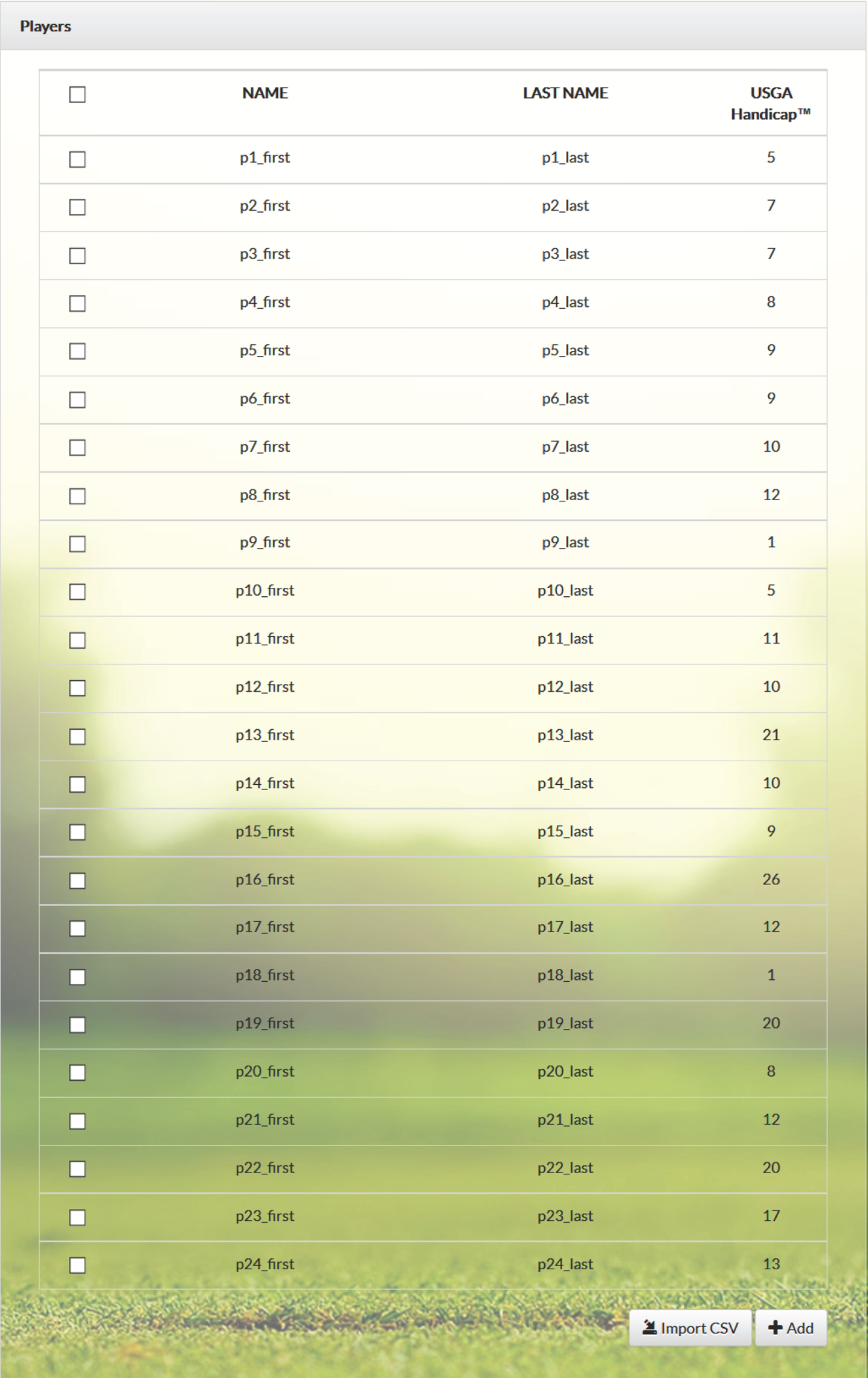
Player List Input. The primary input is a text file of csv (comma separated values) of players as shown in Table 11. The header line is required and the commas are also required. The last name is optional, so the first entry could be “first name,, 5" and only the first name is used. The list can be input from a file by clicking on the  button. This populates the player list as shown in the Figure 1 below.
Table 11
Player list input
| name, lastname, handicap |
| p1_first, p1_last, 5 |
| p2_first, p2_last, 7 |
| p3_first, p3_last, 7 |
| p4_first, p4_last, 8 |
| p5_first, p5_last, 9 |
| p6_first, p6_last, 9 |
| p7_first, p7_last, 10 |
| p8_first, p8_last, 12 |
| p9_first, p9_last, 1 |
| p10_first, p10_last, 5 |
| p11_first, p11_last, 11 |
| p12_first, p12_last, 10 |
| p13_first, p13_last, 21 |
| p14_first, p14_last, 10 |
| p15_first, p15_last, 9 |
| p16_first, p16_last, 26 |
| p17_first, p17_last, 12 |
| p18_first, p18_last, 1 |
| p19_first, p19_last, 20 |
| p20_first, p20_last, 8 |
| p21_first, p21_last, 12 |
| p22_first, p22_last,20 |
| p23_first, p23_last, 17 |
| p24_first, p24_last, 13 |
Fig. 1
Importing the csv data file to the website.
Once entered, the list may be edited manually by adding and deleting players. Deletes are done by clicking the box to the left of a player’s name and then clicking the  button that appears at the bottom of the list after one or more players is selected for deletion. Additions are made using the
  button.
Golf Director Choices. The main web site page has a bar of buttons for the choices of golf director presented in Figure 2.
Fig. 2
The menu of golf director choices.

1. Number of Teams has a drop down menu (or the number can be entered directly). If the number of players is a multiple of the number of teams, then the teams will be of the same size. However, the simulator can handle teams of unequal sizes. For example if there are 13 players and 4 teams, there will be three teams of 3 players and one with 4.
2. The next drop down menu allows the choices of 1, 2 or 3 best ball net scores of players to be counted toward the team score on each hole.
3. The third drop down menu is for the number of simulations. The menu allows up to 10, 000 scenarios, but 1, 000 is usually sufficient. A greater number of scenarios should generally lead to more accurate probability estimates.
4. The final menu button is the handicap allowance for each player, from full handicap, 90% of handicap, 80% of handicap etc., down to No handicap allowance. (The USGA recommends 100% (full) handicaps for fourball match play and 90% for fourball stroke play.)
 starts the simulator. While running, changes cannot be made and the screen is grayed out. The final team score is the sum of the best ball totals for 18 holes. For the 24-player example above, a typical choice would be 6 teams, 2 best balls net, 2, 000 simulations and full handicap allowance. Ideally, the team probabilities to win would be one-sixth (≈16.7%) for each team. Figure 3 presents the simulator output with these choices for the data file above.
Fig. 3
Results of assignment of 24 players in 6 teams. Each team is scored based on 2 best balls, full handicap adjustment is applied.
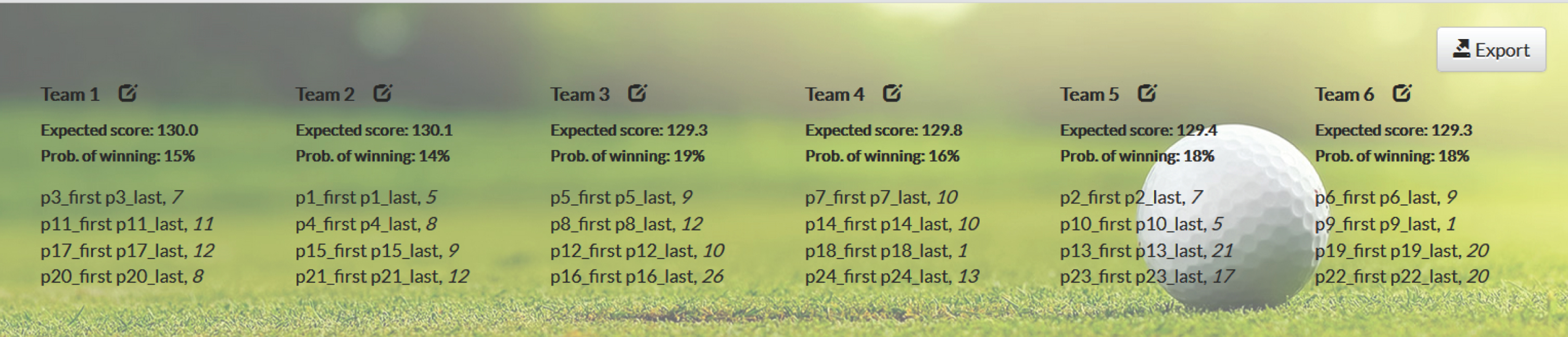
The simulator has determined an assignment of players to teams with a probability to win range of 14% – 19%. The expected score range is 129.3 – 130.1, showing that the teams are fairly assigned. Note also that, when the expected scores are not as close as in this example, the golf director could decide to give team strokes to those with higher expected scores.
Manual Override.The golf director may wish to change the assignments and have the software determine the new probabilities. For example, consider exchanging the 12-handicap player on Team 2 with the 9-handicap player on Team 3. The swap can be done by clicking on the small edit box beside Team 2 which opens a window for making the exchange. Figure 4 is the window with the entries made. To complete the exchange, click  . The assignments are then shown in Figure 5.
Fig. 4
Swap menu dialog.
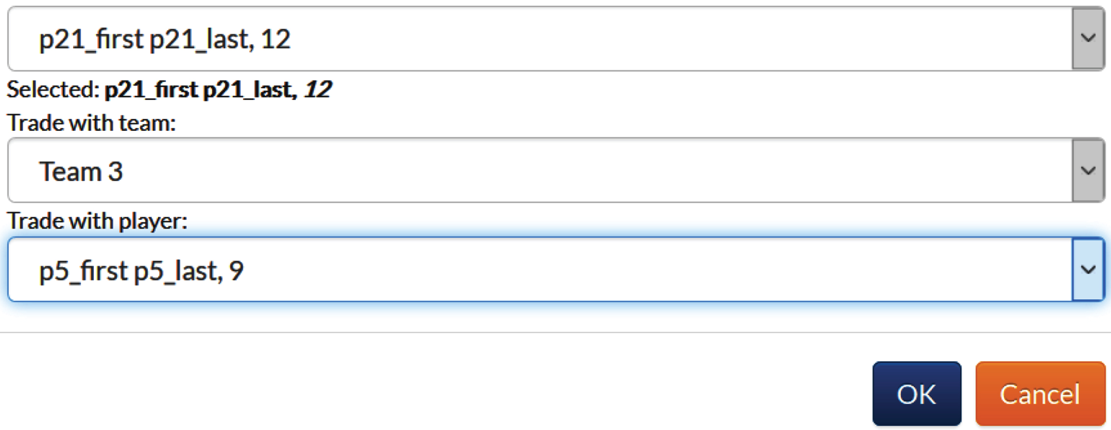
Fig. 5
Teams allocation after a swap is made.
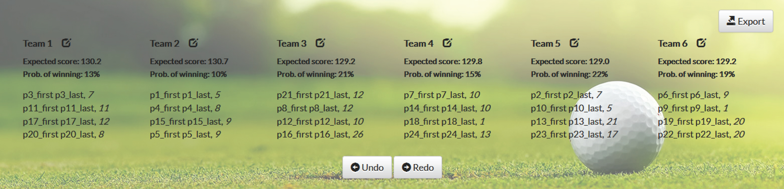
This action has resulted in a worse set of teams because Team 2 now has only a 10% chance of winning while the strongest team still wins with probability 22%. Nevertheless, such manual overrides may help to come up with more preferred team allocations and help to deal with issues such as two players asking to be on the same team. (Of course, it is a matter of judgment as to whether the resulting probabilities are acceptable for the competition.) The  button takes the assignments back to where they were and the
  button provides toggling between the two assignments.
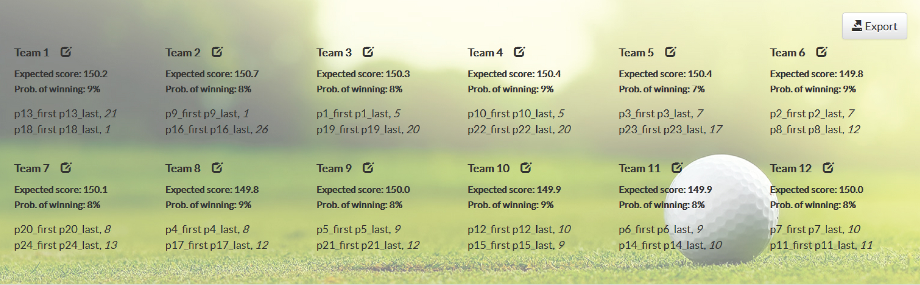
Two player teams and individual expected scores. A natural question is how the simulator works with 2–player teams. In the case of this example, the Number of Teams would be changed to 12 since there are 24 players. Figure 6 shows what happens with 1–best ball for each team and using full handicaps. If there are 2–best balls per team the probability range is similar as is shown in the Figure 7.
Fig. 6
Results of 1-best ball allocation of 24 players into two-player teams.
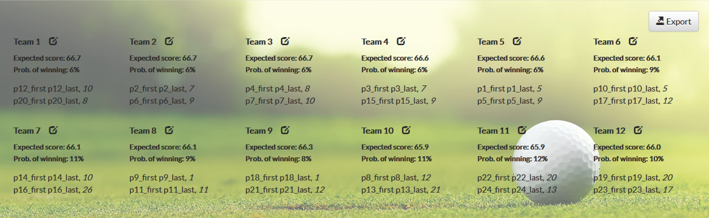
Fig. 7
Results of 2-best ball allocation of 24 players into two-player teams.
Additionally, note that if the number of teams is equal to the number of players, the individual expected scores will be, of course, the same as derivable from the distributions.
To further illustrate the web site software consider the following examples taken from real instances of golf groups.
Example 1: twelve players with handicaps 5, 5, 7, 7, 8, 9, 9, 10, 11, 15, 16, 17.
Since there are twelve players, the golf director could form six, four or three teams of sizes 2, 3, or 4, respectively. The following tables show team assignments (after 10, 000 simulations with full handicaps being used) in the first column, followed by number of Best Balls used, expected team scores (relative to par 72) and the team win probabilities. First, consider creating matches of twosomes, i.e., six 2-player teams. The team fairness results are presented in Table 12. So, if six 2-player teams with full handicaps being used is the choice, this example shows that it more fair to count only 1 best ball rather than 2 best balls. This is intuitively clear since all player scores, good and bad, count in the latter case. The golf director can also vary the number of teams. Tables 13 and 14 show the results for three and four teams.
Table 12
Example 1, results for six 2-player teams
| # Best Balls | Teams | Expected Scores | Win Probabilities (%) |
| 1 | 5, 17 | +4.4 | 16.0 |
| 5, 16 | +4.0 | 18.0 | |
| 7, 15 | +5.1 | 11.0 | |
| 7, 11 | +3.7 | 21.0 | |
| 8, 10 | +4.0 | 18.0 | |
| 9, 9 | +4.1 | 16.0 | |
| 2 | 5, 16 | +26.9 | 10.0 |
| 5, 17 | +28.1 | 8.0 | |
| 7, 15 | +28.1 | 7.0 | |
| 7, 11 | +23.8 | 24.0 | |
| 8, 10 | +23.9 | 24.0 | |
| 9, 9 | +23.6 | 27.0 |
Table 13
Example 1, results for three 4-player teams
| # Best Balls | Teams | Expected Scores | Win Probabilities (%) |
| 2 | 5, 9, 11, 15 | +6.1 | 32.0 |
| 5, 8, 10, 17 | +5.7 | 34.0 | |
| 7, 7, 9, 16 | +5.7 | 34.0 |
Table 14
Example 1, results for four 3-player teams
| # Best Balls | Teams | Expected Scores | Win Probabilities (%) |
| 2 | 5, 10, 15 | +13.1 | 24.0 |
| 5, 9, 17 | +13.1 | 24.0 | |
| 7, 7, 16 | +13.0 | 25.0 | |
| 8, 9, 11 | +12.6 | 27.0 |
These teams show very similar expected scores and provide a narrowed range of win probabilities compared with the six 2-player teams option. Of the four options given, the best, with respect to the ranges of win probabilities and the expected scores, is three 4-player teams. However, the golf director might prefer four 3-player teams for some other reason (such as speed of play) and the results indicate that this would be a reasonable choice.
Example 2: twelve players with handicaps 4, 4, 9, 9, 10, 13, 14, 16, 17, 19, 19, 22.
This example also has 12 golfers but the handicap range is wider, making the problem of arranging a fair game more difficult. Table 15 below shows the six team allocation results.
Table 15
Example 2, results for six 2-player teams
| # Best Balls | Teams | Expected Scores | Win Probabilities (%) |
| 1 | 4, 19 | +4.0 | 39.0 |
| 4, 22 | +4.4 | 34.0 | |
| 9, 17 | +7.1 | 9.0 | |
| 9, 19 | +7.6 | 6.0 | |
| 10, 16 | +7.5 | 7.0 | |
| 13, 14 | +8.3 | 5.0 | |
| 2 | 4, 19 | +29.2 | 36.0 |
| 4, 22 | +32.5 | 15.0 | |
| 9, 17 | +32.6 | 15.0 | |
| 9, 19 | +34.7 | 8.0 | |
| 10, 16 | +32.5 | 15.0 | |
| 13, 14 | +33.5 | 11.0 |
Whether a 1 or 2 best ball game is used, the win probabilities range for six-team allocation is large. For 1 best ball, the teams with the two low handicappers have a definite advantage. With 2 best balls the middle handicap teams gain some advantage, but the (4, 19) team remains dominant. Thus, six 2-player teams is not a good option.
The final tables 16, 17 give the results when 4- and 3-player teams are assigned and 2 best balls are used. It is clear that these two options are better choices because the win probability ranges, as well as the expected score ranges, are much smaller.
Table 16
Example 2, results for three 4-player teams
| # Best Balls | Teams | Expected Scores | Win Probabilities (%) |
| 2 | 4, 13, 16, 19 | +10.3 | 34.0 |
| 4, 10, 19, 22 | +10.4 | 33.0 | |
| 9, 9, 14, 17 | +10.3 | 33.0 |
Table 17
Example 2, results for four 3-player teams
| # Best Balls | Teams | Expected Scores | Win Probabilities (%) |
| 2 | 4, 17, 19 | +18.0 | 25.0 |
| 4, 16, 22 | +18.8 | 20.0 | |
| 9, 13, 14 | +17.7 | 28.0 | |
| 9, 10, 19 | +17.8 | 27.0 |
Example 3: Unequal team sizes.
One difficulty for golf directors is when the number of players is (say) a prime number so that having teams of the same size ≥2 is not possible. This can be especially frustrating when a competition is arranged and then, at the last minute, some players drop out or new ones want to be added.
When this occurs the golf director can run the simulations trying different parameters for the new set of players. There is also a possibly easier alternative. Suppose the 6 teams in Figure 1 have been arranged and player 24 drops out. With that deletion, the simulation is rerun and produces 5 teams of 4 and one team of 3 with (typical) results such as: probabilities of winning are equal to 0.18, 0.22, 0.20, 0.21, 0.17, 0.02. So the range of probabilities is acceptable for 5 teams but the team of 6 has only a 2% chance to win. However, the output of expected scores is 129.8, 129.0, 129.3, 129.2, 130.1, 136.4 and the golf director can use personal judgement decide that the team 6 actual score will be reduced by up to 6 stokes, i.e., the team will receive a handicap that is deemed equitable.
Importing the csv data file to the website.
The menu of golf director choices.
Acknowledgments
Partick Siegbahn’s Master’s thesis first addressed fairness in the fourball game and he developed the score distributions by player handicap using a data base provided by Golfnet.com. Also, Patrick Fieldson developed a desktop system for an earlier version of the golf director problem.
References
1 | Ball, M. & Halper, R. , (2009) , Scramble Teams for the Pinehurst Terrapin Classic, Journal of Quantitative Analysis in Sports 5: (2). |
2 | Chan, T. C. , Madras, D. & Puterman, M. L. , (2018) , Improving Fairness in Match Play Golf Through Enhanced Handicap Allocation, Journal of Sports Analytics 4: (4), 251–262. |
3 | Dear, R. G. & Drezner, Z. , (2000) , Applying Combinatorial Optimization Metaheuristics to the Golf Scramble Problem, International Transactions in Operational Research 7: (4-5), 331–347. |
4 | Grasman, S. E. & Thomas, B. W. , (2013) , Scrambled Experts: Team Handicaps and Win Probabilities for Golf Scrambles, Journal of Quantitative Analysis in Sports 9: (3), 217–227. |
5 | Hurley, W. & Sauerbrei, T. , (2015) , Handicapping Net Best-Ball Team Matches in Golf, Chance 28: (2), 26–30. |
6 | Lewis, A. J. , (2005) , A. J., Handicapping in Group and Extended Golf Competitions, IMA Journal of Management Mathematics 16: (1), 151–160. |
7 | Pavlikov, K. , Hearn, D. & Uryasev, S. , (2014) , The Golf Director Problem: Forming Teams for Club Golf Competitions, in ‘Social Networks and the Economics of Sports’, Springer, pp. 157–170. |
8 | Pollard, G. & Pollard, G. , (2010) , Four Ball Best Ball, Journal of Sports Science and Medicine 9: (1), 86–91. |
9 | Pollock, S. M. , (1974) , A Model for Evaluating Golf Handicapping, Operations Research 22: (5), 1040–1050. |
10 | Ragsdale, C. T. , Scheibe, K. P. & Trick, M. , (2008) , Fashioning Fair Foursomes for the Fairway (Using a Spreadsheet-based DSS as the Driver, Decision Support Systems 45: (1), 997–1006. |
11 | Siegbahn, P. & Hearn, D. , (2010) , A Study of Fairness in Fourball Golf Competition, in ‘Optimal Strategies in Sports Economics and Management’, Springer, pp. 143–170. |
12 | Tallis, G. M. , (1994) , A Stochastic Model for Team Golf Competitions with Applications to Handicapping, Australian Journal of Statistics 36: (1), 257–269. |


