
Are strategies for success different in test cricket and one-day internationals? Evidence from England-Australia rivalry1
Abstract
The paper utilizes the entire cricketing data between England and Australia–Test and one-day international (ODI) matches played between 1877-2015 and 1971-2015, respectively–to provide an econometric perspective on the England-Australia rivalry. We employ the production function approach of Schofield (1988) and model Test match outcomes (loss, draw or win) using an ordinal probit model and ODI outcomes (loss or win) using a binary probit model. The results show that input measures critical to winning are different for the two formats and consequently a team should adopt different strategies in Test and ODI matches. We further show that influences which are perceived as important to match outcomes, including electing to bat first after winning the toss and effect of weather conditions, do not have any statistical support. However, there is strong evidence that England is at a disadvantage while playing a Test match in Australia. Besides, we find that home bias as typically defined in the literature may not necessarily indicate favoritism by umpires. The estimated models fit well and correctly predict about 70% of Test match outcomes and 95% of ODI outcomes.
1Introduction
Cricket is a popular team sport with readily available historical data, but quantitative analysis of cricket lags far behind other team sports including baseball, basketball and soccer. Most analysis on cricket has been recent and typically based on the production function approach, where a cricketing team is viewed as a firm that produces outputs (wins/points) based on inputs such as batting, bowling and fielding performances by the players (Schofield, 1988). This approach is common to all professional team sports within the sports economics literature and has its foundation in the pioneering work of Rottenberg (1956), Neale (1964) and Demmert (1973). Some articles on cricket that utilize the production function approach to model match outcomes include Bairam et al. (1990), Brooks et al. (2002) and Cannonier et al. (2015). Many studies have also focused on specific aspects related to the game including winning the toss and electing to bat first (Dawson et al., 2009; De Silva and Swartz, 1998; Forrest and Dorsey, 2008), home team advantage (De Silva and Swartz, 1998; Morley and Thomas, 2015), home bias in officiating matches (Crowe and Middeldorp, 1996; Sacheti et al., 2016b), distribution of runs scored and batting strategy in Test cricket (Scarf et al., 2011), attendance in Test matches (Bhattacharya and Smyth, 2003), attendance in ODIs (Morley and Thomas, 2007; Sacheti et al., 2014, 2016a), ratings of cricket teams (Allsopp and Clarke, 2004) and cricket’s decision review system (Borooah, 2016). Some other studies have employed sophisticated modeling techniques to evaluate optimal scoring rates (Clarke, 1988), player performance (Johnston et al., 1993), simulate in-play outcomes in ODIs (Sargent and Bedford, 2012), batting performance in ODIs (Koulis et al., 2014) and declaration guidelines in Test cricket (Perera et al., 2014).
The list of papers mentioned above, although incomplete, provides a glimpse on the nature of studies undertaken with respect to Test and ODI cricket in sports economics. However, most of these papers and other exercises have generally used cricketing data for multiple teams spanning a short period of time and none to our knowledge have utilized the complete historical data of any cricketing series or concentrated on the rivalry between two nations. Our present inquiry takes a step in this direction and we explore the bilateral cricketing rivalry between England and Australia using complete historical data–Test and ODI matches played between 1877-2015 and 1971-2015, respectively. We choose England because it is the birthplace of cricket and has played a noticeable role in shaping the world cricket through the participation of international players in county cricket. On the other hand, Australia is selected given its inspiring dominance on world cricket in the last three decades. Besides, both the countries are among the oldest playing nations; in fact, the first officially recognized Test match (1877, Melbourne Cricket Ground) and ODI (1971, Melbourne Cricket Ground) were played between England and Australia. Two characteristics pertinent to the English and Australian cricket make their case particularly interesting. First, the Ashes Test series is an emblem of intense rivalry and is arguably the most celebrated Test series in the world. Second, while England has never won an ODI world cup, Australia has won 5 out of 11 (in 1987, 1999, 2003, 2007 and 2015). The contribution of these two countries has been unique to the development of cricket, and hence an analysis of their winning strategies in Test and ODI matches can be a useful benchmark for other cricketing teams.
The playing strategies that a team adopts largely depend on the rules of the game, and interestingly, both Test and ODIs have gone through several modifications largely driven to renew spectator interest and generate revenues. This has led to the adoption of shorter and more result oriented formats over time. For instance, Test cricket in its earliest days was not constrained by time (henceforth referred to as timeless) and only ended when either of the playing teams won, and hence, declaration of an innings was an unpopular practice. The timeless format was abandoned in the 1930’s and declaration along with follow-on became the accepted practice in the newer five-day format of Test cricket. However, the multi-day nature of Test matches was not spectator friendly and led to the evolution of limited over ODIs in the 1970’s. Currently, both Test matches and ODIs co-exist along with an even shorter and more recent format named Twenty20 (T20), which only lasts about 3–4 hours.
We anticipate that different rules in Test and ODI cricket, summarized in Table 1, will lead to different combinations of performance inputs for a successful match outcome in this bilateral rivalry. Therefore, an important goal is to identify the contribution of various performance inputs on match outcomes and find differences in winning strategy, if any, for Test and ODI matches. We employ the production function approach and consider the English team as the firm of interest with its success (i.e., production output) expressed as a function of batting, bowling and a host of other factors/inputs. The outcomes from a Test match, loss, draw or a win, are ordered and discrete and analyzed within an ordinal probit model. In contrast, ODI matches typically resulting in loss or win is studied using a binary probit model. The results show that different playing strategies are essential for winning a Test/ODI match. Further, we set several orthodox notions, such as disadvantage associated with playing abroad, batting first after winning the toss and first innings lead, to statistical investigation and come up with interesting results. We also investigate for potential bias by match officials (or umpires) in favor of the home team and the effect of shorter formats on the longer format of the game. For each model, we also compute diagnostic measures and show that the proposed models fit well with a reasonably good predicting power.
Table 1
Characteristics of Test and ODI cricket matches
| Test Match | ODI |
| Maximum duration of a Test match is 5 days. However, duration varied from 3 days to no upper bound in earlier days. | ODI matches have a maximum duration of 1 day. |
| Test matches have no limitation on number of overs, where an over consists of 6 balls in the modern format. In older versions, number of balls per over ranged from 4 to 8 balls. | ODI is a limited over cricket. Currently, each team bowls 50 overs, but earlier versions varied from 40 to 60 overs. Similar to Test matches, an over consists of 6 balls (8 balls) in the modern (older) version. |
| A Test match typically consists of two innings per team, where an inning concludes if the batting team loses all 10 wickets (all out) or team captain declares to close the inning. | An ODI match consists of one innings per team and an inning concludes if the batting team is all out or exhausts the 50 overs of play. |
| A team wins if the aggregate score is higher than the aggregate score of its opponent, irrespective of the number of innings played. The match results in a draw if the aggregate score is same for both teams or if after 5 days of play, either one or both teams have wickets due for batting. | A team wins if it scores more runs than its opponent. If both teams score equal runs, the result is a tie, a rare occurrence. |
The remaining article is organized as follows. Section 2 explains the data and the construction of variables, presents summary statistics and performs a set of t-tests to examine differences in variables over time and between teams. Section 3 presents different models for Test and ODI cricket, examines orthodox notions and explains the effect of different inputs on a match outcome. Section 4 concludes and presents a brief discussion on strategic implications of our findings.
2Data
We collect data on 331 Test and 131 ODI cricket matches played between England and Australia for the period 1877-2015 and 1971-2015, respectively, from the publicly available database http://www.cricketarchive.com/. There were an additional 13 Test matches that we do not consider in the current study, since 3 were abandoned and 10 were declared draw before completion. Similarly, information for 8 ODI matches is not used, as they were either a tie, canceled mid-way or abandoned. Besides, amongst the 131 ODI matches, we judiciously utilize information on 8 matches played in neutral venues. This is done so as to examine systematic home bias by match umpires.
The literature on modeling the outcome of a cricket match, as mentioned in Section 1, has followed the production function approach, where the match outcome is the output and performances in batting, bowling and other relevant match characteristics (e.g., toss wins, batting first) are used as inputs. In our study, we model the outcome of a match from England’s perspective and the outcome for Australia is simply the reverse of England’s outcome, except for draws in Test matches when outcomes are identical. The independent variables used in the study are presented in Table 2 and the definitions of common variables remain unchanged for both Test matches and ODIs. The only difference is that the batting and bowling inputs in Test matches are defined over two innings as opposed to a single inning in ODIs. Such an aggregation is required for Test matches since, occasionally, a team plays one innings while the opponent plays two innings. The following paragraphs explain the rationale and present the summary statistics of all the variables used in different models.
Table 2
Variable definition
| VARIABLE | DESCRIPTION |
| EngRPO (AusRPO) | Runs per over by England (Australia) in a Test match/ODI. |
| EngRPW (AusRPW) | Runs per wicket by England (Australia) in a Test match/ODI. |
| EngAttackBat (AusAttackBat) | Proportion of runs scored in fours and sixes by England (Australia) in a Test Match/ODI. |
| EngTeamQuality (AusTeamQuality) | Proportion of Test/ODI win (or draw for Test match only) by England (Australia) against all teams in a year, except Australia (England). |
| EngWinToss | Indicator variable, equals 1 if England wins the toss. |
| EngBatFirst | Indicator variable, equals 1 if England elects to bat first. |
| VenEngland | Indicator variable, equals 1 if match venue is England. |
| VenAustralia | Indicator variable, equals 1 if match venue is Australia. |
| HomeBias | Difference in number of leg before wickets (LBW) between the visiting team and the home team. Not defined for neutral venues. |
| ThreeFourDay | Indicator variable for Test matches of length 3 or 4 days. |
| FiveSixDay | Indicator variable for Test matches of length 5 or 6 days. |
| Weather | Indicator variable, equals 1 if Test match is weather affected. |
| FirstInnLead | Surplus/deficit in first inning runs scored by England compared to Australia (applicable only for Test matches). |
| Innings4 | Proportion of England versus Australia Test matches in a year with fourth innings score greater than or equal to 275 runs. |
| Score275 | Proportion of England versus Australia ODI matches in a year with score greater than or equal to 275 runs. |
| T20I | Indicator variable, equals 1 if the match was played post the introduction of T20s. |
We define batting input (and bowling input) in two different ways to make our analysis robust to the use of different definitions of variables. In the first or ‘traditional’ approach, we separate batting inputs according to the intent of the batting team (Schofield, 1988). Specifically, runs scored per over (aka run rate) by England (EngRPO) is used to capture the attacking intent, and runs scored per wicket by England (EngRPW) is used to capture the defensive intent. The intuition underlying this categorization is that, given fixed runs per wicket, a higher run rate would demonstrate a team’s ability to score runs quickly by hitting fours (or boundaries) and sixes. Similarly, given a fixed run rate, higher runs per wicket would demonstrate the intent of preventing dismissal from the field. Note that aggressive batting comes with a trade off, as it increases the risk of losing wickets quickly. Run rate as a surrogate of batting strategy has been employed in several papers including Brooks et al. (2002), Scarf et al. (2011) and Cannonier et al. (2015). In the second approach, we use the proportion of runs scored in fours and sixes by England (EngAttackBat) instead of EngRPO. This ‘modern’ approach, introduced by Cannonier et al. (2015), is more appropriate and particularly relevant to ODIs because in limited-over matches, if both the teams use all the allocated overs, the team with higher RPO wins by definition.
Similarly, we utilize two different approaches to define bowling variables for England. The first approach uses runs scored per over by Australia (AusRPO) and runs scored per wicket by Australia (AusRPW) to capture the defensive and attacking bowling intent, respectively (Brooks et al., 2002; Cannonier et al., 2015). The underlying intuition is similar too. Given fixed runs per wicket, a lower run rate of the Australian team would indicate the English team’s desire to minimize Australia’s score without dismissing all the Australian batsmen. Likewise, given a fixed run rate, lower runs per wicket of the Australian team would indicate the English team’s desire to bowl and dismiss all the batsmen. The second approach measures English team’s defensive bowling intent through the proportion of runs scored in fours and sixes by the Australian team (AusAttackBat). The lower this proportion, the slower is Australia’s run accumulation in the game. Note that AusAttackBat indicates a defensive bowling intent as opposed to an attacking bowling intent, as it measures containment of runs and not player dismissals. Apart from the batting and bowling variables, one may also include variables indicating fielding quality as measured by the number of catches and run-outs. However, we refrain from doing so due to the aggregate nature of fielding variable and the difficulty in knowing how much of a role batting stance (aggressive or non-aggressive) and bowling performance played in influencing this variable.
To measure England’s (Australia’s) overall team quality, we use the annual proportion of wins against all teams, except Australia (England). The idea is simple; if an English team is winning against all other national teams, it is more likely to win against Australia and vice-versa. Note that our definition of team quality counts the match in the year when it starts. The covariates also include indicator variables for toss outcome (from England’s perspective) and whether England bats first. An interaction term between the two indicators is also included (in the baseline models) since choosing to bat first after winning a toss is a widely accepted strategy. In fact, captains have been bitterly criticized for losing a match, when they won the toss and elected to bowl first. Examples include the criticism faced by Ricky Ponting and Saurav Ganguly following the loss in the second Test of the 2005 Ashes series and the 2003 World Cup final, respectively. So, it is important to examine the utility of this strategy.
We also include location indicator variables for matches played in England, neutral venues and Australia. Matches played in England are treated as the base category and omitted from all models. In this context, we see that only 8 ODI matches, but no Test matches, have been played in neutral venues. The location indicator can be a decisive factor because teams are more likely to bat first after winning the toss in the hard and bouncy pitches of Australia as opposed to the cold and wet English conditions. This is also borne out in the data. In the 177 Test matches played in Australia, England won the toss in 77 Test matches and chose to bat first on 59 occasions i.e., 76.62 percent. Similarly, amongst the 65 ODI matches that have been played in Australia, England won the toss in 38 ODI matches and elected to bat first in 28 of them, i.e., 73.68 percent. Hence, we include an interaction term for the three variables: matches played in Australia, winning the toss and electing to bat first. We also include a variable ‘HomeBias’ to examine systematic bias, if any, by umpires in favor of home teams has a significant effect on match outcomes. The inclusion of ‘HomeBias’ draws inspiration from earlier works ( Crowe and Middeldorp, 1996; Ringrose, 2006; Sacheti et al., 2015), where they found some evidence of umpires favoring the home team in officiating matches. Note that since HomeBias is not well defined for neutral locations and the number of ODI matches played in neutral venues is small, we restrict the use of ODI matches played in neutral venues to the baseline models only.
We also include some format specific variables for Test and ODI matches. In Test matches, maximum number of days (i.e., length or duration) has varied over time, so we include indicator variables for length of a Test match (see Table 2). We expect the length to be inversely proportional to the probability of a draw and the data support our hypothesis. It is observed that 18 out of 45 (40%) three-day matches, 5 out of 10 (50%) four-day matches, 55 out of 172 (31.98%) five-day matches, 5 out of 24 (20.83%) six-day matches, and 0 out of 80 (0%) of timeless matches ended up in a draw. Similarly, we include an indicator variable to capture the effect of weather interruptions in Test matches; motivation being that a temporary suspension of a match increases the probability of a draw. Note that the effect of match interruptions comes into play only if the number of playing days is fixed and should not matter in timeless matches. The data again corroborate this assertion, as about 69% of weather affected fixed length Test matches ended up in a draw. The number of playing days and weather interruptions are not so relevant for ODI matches as they do not span more than a day. In Test matches, first innings lead is important and plays an important role in a match outcome. We also create indicator variables to measure the impact of one format of the game on the other. In particular, a variable ‘Innings4’, defined in Table 2, is created to measure the impact of ODI or T20 on Test cricket depending on the time period. Similarly, we define a variable ‘Score275’ in Table 2 to capture the effect of T20 on ODI matches.
2.1Data summary: Test match
We next present the descriptive statistics for Test matches in Table 3 corresponding to nine different time periods to get an idea about different issues of interest. The first three time periods (1877-1939, 1940-1970 and 1971-2015) cover the entire historical data, and the data summary gives a sense of chronological developments. The period 1877-1939 corresponds to the span when timeless format and three-four day format were popular in Test cricket. Both formats were abandoned in 1939 and the duration of Test matches was fixed to either five or six days. The third period 1971-2015 coincides with the era post the introduction of ODI matches. The next two time periods present the summary statistics pre (1971-2004) and post (2005-2015) the introduction of T20 cricket. This classification is interesting since it is often argued that the rate of scoring runs in Test and ODI matches have increased following the introduction of T20 cricket. The sixth and seventh time periods present the summary statistics pre (1971-1993) and post (1994-2005) the introduction of one neutral umpire in the Test cricket to assess differences, if any, related to home bias. Similarly, the eight and ninth time periods refer to periods prior to (1971-2001) and post (2002-2015) the introduction of two neutral umpires in Test cricket.
Table 3
Summary statistics for Test matches
| 1877-1939 | 1940-1970 | 1971-2015 | 1971-2004 | 2005-2015 | 1971-1993 | 1994-2015 | 1971-2001 | 2002-2015 | ||||||||||
| Variable | mean | std | mean | std | mean | std | mean | std | mean | std | mean | std | mean | std | mean | std | mean | std |
| EngRPO | 2.60 | 0.45 | 2.30 | 0.34 | 2.97 | 0.59 | 2.83 | 0.52 | 3.39 | 0.60 | 2.76 | 0.53 | 3.24 | 0.56 | 2.82 | 0.53 | 3.34 | 0.58 |
| EngRPW | 32.81 | 20.67 | 31.85 | 11.56 | 32.29 | 15.72 | 31.28 | 13.77 | 35.19 | 20.25 | 32.93 | 14.47 | 31.53 | 17.21 | 31.44 | 13.98 | 34.33 | 19.30 |
| EngAttackBat | 0.30 | 0.13 | 0.37 | 0.11 | 0.45 | 0.09 | 0.44 | 0.08 | 0.50 | 0.09 | 0.43 | 0.09 | 0.49 | 0.09 | 0.43 | 0.09 | 0.50 | 0.09 |
| AusRPO | 2.71 | 0.66 | 2.54 | 0.48 | 3.14 | 0.62 | 2.97 | 0.59 | 3.61 | 0.44 | 2.76 | 0.41 | 3.60 | 0.51 | 2.91 | 0.53 | 3.68 | 0.46 |
| AusRPW | 29.05 | 14.32 | 35.47 | 17.42 | 40.48 | 24.52 | 40.58 | 26.07 | 40.19 | 19.77 | 39.68 | 25.86 | 41.44 | 22.97 | 40.10 | 26.53 | 41.38 | 19.19 |
| AusAttackBat | 0.29 | 0.14 | 0.39 | 0.10 | 0.44 | 0.09 | 0.42 | 0.09 | 0.50 | 0.06 | 0.40 | 0.08 | 0.48 | 0.08 | 0.41 | 0.09 | 0.50 | 0.07 |
| EngTeamQuality | 0.65 | 0.25 | 0.76 | 0.23 | 0.73 | 0.21 | 0.72 | 0.22 | 0.76 | 0.16 | 0.70 | 0.25 | 0.76 | 0.15 | 0.70 | 0.23 | 0.78 | 0.15 |
| AusTeamQuality | 0.57 | 0.17 | 0.72 | 0.25 | 0.76 | 0.20 | 0.76 | 0.19 | 0.78 | 0.25 | 0.74 | 0.21 | 0.79 | 0.19 | 0.75 | 0.19 | 0.80 | 0.22 |
| HomeBias | 0.19 | 1.36 | 0.41 | 1.62 | 0.43 | 2.25 | 0.15 | 2.19 | 1.23 | 2.26 | 0.17 | 2.13 | 0.75 | 2.37 | 0.07 | 2.13 | 1.27 | 2.35 |
| FirstInnLead | 28.78 | 184.45 | -44.34 | 172.39 | -44.01 | 185.88 | -54.42 | 168.31 | -14.26 | 229.01 | -33.14 | 171.04 | -57.20 | 203.09 | -49.49 | 168.29 | -35.73 | 224.39 |
| Innings4 | 0.17 | 0.28 | 0.06 | 0.14 | 0.15 | 0.22 | 0.14 | 0.22 | 0.18 | 0.22 | 0.15 | 0.24 | 0.16 | 0.20 | 0.16 | 0.23 | 0.15 | 0.21 |
| count | per | count | per | count | per | count | per | count | per | count | per | count | per | count | per | count | per | |
| EngWinToss | 66 | 48.89 | 32 | 52.46 | 64 | 47.41 | 44 | 44.00 | 20 | 57.14 | 35 | 47.30 | 29 | 47.54 | 40 | 42.11 | 24 | 60.00 |
| EngBatFirst | 65 | 48.15 | 34 | 55.74 | 68 | 50.37 | 51 | 51.00 | 17 | 48.57 | 38 | 51.35 | 30 | 49.18 | 48 | 50.53 | 20 | 50.00 |
| VenEngland | 60 | 44.44 | 29 | 47.54 | 65 | 48.15 | 47 | 47.00 | 17 | 48.57 | 36 | 48.65 | 29 | 47.54 | 47 | 49.47 | 22 | 55.00 |
| VenAustralia | 75 | 55.56 | 32 | 52.46 | 70 | 51.85 | 53 | 53.00 | 18 | 51.43 | 38 | 51.35 | 32 | 52.46 | 48 | 50.53 | 18 | 45.00 |
| ThreeFourDay | 55 | 40.74 | 0 | 0.00 | 0 | 0.00 | 0 | 0.00 | 0 | 0.00 | 0 | 0.00 | 0 | 0.00 | 0 | 0.00 | 0 | 0.00 |
| FiveSixDay | 0 | 0.00 | 61 | 100.00 | 135 | 100.00 | 100 | 100.00 | 35 | 100.00 | 74 | 100.00 | 61 | 100.00 | 95 | 100.00 | 40 | 100.00 |
| Timeless | 80 | 59.26 | 0 | 0.00 | 0 | 0.00 | 0 | 0.00 | 0 | 0.00 | 0 | 0.00 | 0 | 0.00 | 0 | 0.00 | 0 | 0.00 |
| Weather | 9 | 6.67 | 15 | 24.59 | 7 | 5.19 | 5 | 5.00 | 2 | 5.71 | 2 | 2.70 | 5 | 8.20 | 5 | 5.26 | 2 | 5.00 |
| England Loses | 57 | 42.22 | 23 | 37.70 | 60 | 44.44 | 45 | 45.00 | 18 | 51.43 | 28 | 37.84 | 32 | 52.46 | 41 | 43.16 | 18 | 45.00 |
| Match Draw | 23 | 17.04 | 27 | 44.26 | 33 | 24.44 | 26 | 26.00 | 15 | 42.86 | 23 | 31.08 | 10 | 16.39 | 26 | 27.37 | 19 | 47.50 |
| EnglandWins | 55 | 40.74 | 11 | 18.03 | 42 | 31.11 | 29 | 29.00 | 7 | 20.00 | 23 | 31.08 | 19 | 31.15 | 28 | 29.47 | 7 | 17.50 |
We begin with the first three time periods in Table 3 and see that runs per over (both EngRPO and AusRPO) decreased during 1940-1970 compared to 1877-1939, but was higher during 1971-2015. Here, we note that Test (and ODI) matches during early days sometimes had 4, 5 or 8 balls per over, so we have standardized and reported runs per 6 balls an over. Runs per wicket for England (EngRPW) decreased to 31.85 (from 32.81) during 1940-1970, but increased to 32.29 during 1971-2015. In contrast, runs per wicket for Australia (AusRPW) shows an increasing trend and stood at 40.48 between 1971-2015. Over the periods, the proportion of runs scored in fours and sixes by both the countries have increased which indicates that batting has become more attacking, especially during 1971-2015, possibly reflecting the influence of fast paced ODI and T20 cricket. The proportion of Test match wins or draws by Australia (AusTeamQuality) have steadily increased, but that of England (EngTeamQuality) increased from 0.65 during 1877-1939 to 0.76 during 1940-1970, but decreased to 0.73 during 1971-2015. Home bias as defined in Table 2 is positive, but the standard deviations are large. The first innings lead (FirstInnLead) averaged at 28.78 during 1877-1939, but dropped to less than -44 in the subsequent time periods. This clearly shows a better performance by the Australian team.
Table 4
The table presents the difference in mean/proportion test for some selected Test-match variables across time periods. In the first panel, the tests correspond to the mean/proportion difference between post (1971-2004) and prior (1940-1970) to the introduction of ODI’s, and post (2005-2015) and prior (1971-2004) to the introduction of T20 cricket. In the second panel, the tests on mean difference in HomeBias correspond to post and prior to the introduction of one and two neutral umpires. The third panel is similar to the second panel, but considers the period 1971-2015 instead of 1940-2015
| (1971-2004)-(1940-1970) | (2005-2015)-(1971-2004) | |||||
| Variable | diff | se | t-stats | diff | se | t-stats |
| EngRPO | 0.53 | 0.07 | 7.06 | 0.56 | 0.11 | 5.28 |
| EngAttackBat | 0.07 | 0.01 | 4.29 | 0.06 | 0.02 | 3.77 |
| AusRPO | 0.43 | 0.09 | 4.81 | 0.63 | 0.11 | 5.83 |
| AusAttackBat | 0.03 | 0.01 | 2.05 | 0.08 | 0.02 | 4.96 |
| EngRPW | -0.57 | 2.11 | 0.27 | 3.91 | 3.08 | 1.27 |
| AusRPW | 5.11 | 3.77 | 1.35 | -0.39 | 4.83 | 0.08 |
| Innings4 | 0.08 | 0.05 | 1.34 | 0.04 | 0.09 | 0.43 |
| (1994-2015)-(1940-1993) | (2002-2015)-(1940-2001) | |||||
| HomeBias (In England) | 0.44 | 0.47 | 0.93 | 1.38 | 0.54 | 2.56 |
| HomeBias (In Australia) | 0.50 | 0.42 | 1.18 | 0.77 | 0.48 | 1.61 |
| HomeBias | 0.48 | 0.32 | 1.51 | 1.07 | 0.36 | 2.97 |
| (1994-2015)-(1971-1993) | (2002-2015)-(1971-2001) | |||||
| HomeBias (In England) | 1.10 | 0.56 | 1.99 | 1.97 | 0.59 | 3.34 |
| HomeBias (In Australia) | 0.08 | 0.50 | 0.18 | 0.44 | 0.53 | 0.83 |
| HomeBias | 0.59 | 0.39 | 1.52 | 1.20 | 0.41 | 2.90 |
The second panel in Table 7 presents the counts and percentages of categorical variables. During the first three periods, England won the toss in 66 (48.89%), 32 (52.46%) and 64 (47.41%) Test matches against Australia. The numbers for England batting first closely follow the numbers for England winning the toss. Indicator variables for match venue show that in each of the three periods, less than 50% of the matches have been played in England. As described earlier, the duration of a Test match has varied over time and Table 3 shows that during the last 76 years (1940-2015), Test matches played over 5 or 6 days have gained prominence. Although we have clubbed 5 or 6 days Test matches together, modern Test format is limited to 5 days. This is apparent between 1971-2015 when 132 out of 135 Test matches (i.e., 97.78%) played between England and Australia were of 5 days format. The multi-day nature of a Test match makes it more likely to be affected by weather conditions such as rain. Table 3 shows that 31 (9.37%) Test matches have been affected by weather interruptions during 1877-2015. The last panel of Table 3 presents the match outcomes and it reveals that England has lost (i.e., Australia has won) a larger percentage of Test matches in each of the first three time periods.
Table 5
The table presents paired t-tests to examine differences in RPO and attacking batting in Test matches between Australia and England for three different time periods
| 1940-1970 | 1971-2004 | 2005-2015 | |||||||
| Variable | diff | se | t-stat | diff | se | t-stat | diff | se | t-stat |
| DiffRPO | 0.24 | 0.08 | 3.12 | 0.14 | 0.06 | 2.51 | 0.22 | 0.13 | 1.66 |
| DiffAttackBat | 0.02 | 0.01 | 1.42 | -0.02 | 0.01 | 2.47 | -0.01 | 0.01 | 0.17 |
We next focus on the summary statistics before and after the introduction of T20 cricket i.e., 1971-2004 and 2005-2015. Table 3 shows that both runs per over and proportion of runs scored in fours and sixes increased following the debut of T20 cricket. In particular, EngRPO (AusRPO) increased from 2.83 (2.97) during 1971-2004 to 3.39 (3.61) during 2005-2015 and EngAttackBat (AusAttackBat) increased from 0.44 (0.42) to 0.50 (0.50) between the same periods. Another interesting feature is that the mean first innings lead dropped from -54.42 to -14.26, but the standard deviations are high. Finally, classifying the data as pre and post the introduction of (one or two) neutral umpires shows that mean HomeBias actually increased following the introduction of neutral umpires, which is actually contrary to the expectation.
We have seen in Table 3 that there are some differences in the summary statistics of the variables, however, the differences may or may not be statistically significant. Hence, we conduct difference in mean/proportion tests in Table 4 and paired t-tests in Table 5 to answer some pertinent questions. Both tables report the mean/proportion difference (diff), standard error (se) and t-statistics (t-stats) for each test. The first panel of Table 4 shows that the mean difference in RPO (EngRPO and AusRPO) and the proportion of runs scored in fours and sixes (EngAttackBat and AusAttackBat) are positive and statistically significant. In contrast, the effect on runs per wicket (EngRPW and AusRPW) is statistically insignificant for the considered time periods. This implies that for both England and Australia, the rate of accumulating runs in Test matches increased, indicating that the batting became more attacking following the introduction of ODI cricket and then again following the introduction of T20 cricket. The mean difference in ‘Innings4’ (our measure to capture the effect of faster format on Test cricket) is positive, but not statistically significant.
The second and third panels of Table 4 present extensive test results for the variable HomeBias. In the second panel, we consider the period 1940-2015 and break the sample into pre and post the introduction of one and two neutral umpires. When we split the sample based on one neutral umpire, the mean home bias is positive but statistically insignificant. However, when we split the sample based on two neutral umpires, the mean home bias is positive and statistically significant for the matches played in England, but statistically insignificant for the matches played in Australia. This implies that post the introduction of two neutral umpires, mean difference in LBW decisions has increased for matches played in England. In other words, the visiting Australian team has received more LBW decisions as compared to the English team after the introduction of two neutral umpires. However, no such statistical difference is observed for Test matches played in Australia. The third panel is analogous to the second panel, but considers the period 1971-2015. Results again point to an increase in the mean difference in home bias for the matches played in England, but now the significance holds for both one and two neutral umpires. However, there is no evidence of an increase in mean home bias when matches are played in Australia. Overall, the results on variable HomeBias are robust to changes in time periods.
We also conduct tests for mean difference in home bias by dividing the sample according to match location or venue (not shown in the table). The test results yield that for all matches played in England during the period 1940-2015, mean difference in home bias is 0.61 with a t-statistic of 2.07. The same test over the period 1971-2015 yields a mean difference of 1.21 with a t-statistic of 3.23. This implies that the visiting Australian team received more LBW decisions in England than the English team post the introduction of neutral umpires. This finding is counter-intuitive to the favoritism argument and suggests that one must be careful while interpreting the variable HomeBias. In the current scenario, the positive mean difference in home bias possibly reflects the often cited claim that Australia is not comfortable playing in the turning pitches of England. Moreover, data suggests that the Australian team has failed to make any significant improvement to play in the turning pitches, since the results hold for different time periods.
Lastly, we examine difference in run scoring abilities between Australia and England using paired t-tests for three different time periods: 1940-1970 (i.e., the period after the abolition of timeless Test matches but before the introduction of ODI), 1971-2004 (i.e., the period following introduction of ODI’s but before T20 cricket) and 2005-2015 (i.e., the period following the introduction of T20 cricket). The results from the tests are displayed in Table 5. We see that DiffRPO (defined as AusRPO - EngRPO) is positive and statistically significant for 1940-1970 and 1971-2004, but positive and insignificant for 2005-2015. This implies that Australia’s mean RPO is statistically higher than that of England in the first two periods, but statistically equivalent post the introduction of T20 cricket. However, a look at the variable DiffAttackBat (defined as AusAttackBat - EngAttackBat) gives a completely different picture. The mean difference is statistically insignificant for 1940-1970 and 2005-2015, but negative and significant for 1971-2004. This suggests that for the period 1971-2004, England scored a higher proportion of runs in fours and sixes compared to that of Australia, but for the two other periods the proportions are statistically equivalent.
2.2Data summary: ODI
Table 6
Summary statistics for 123 ODI matches (excludes matches played in neutral venues)
| 1971-2004 | 2005-2015 | 1971-2001 | 2002-2015 | 1971-2015 | ||||||
| Variable | mean | std | mean | std | mean | std | mean | std | mean | std |
| EngRPO | 4.27 | 0.82 | 5.06 | 0.73 | 4.25 | 0.80 | 4.99 | 0.79 | 4.60 | 0.87 |
| EngRPW | 32.08 | 19.95 | 35.50 | 30.08 | 32.36 | 20.25 | 34.79 | 28.87 | 33.52 | 24.69 |
| EngAttackBat | 0.34 | 0.09 | 0.40 | 0.08 | 0.34 | 0.10 | 0.39 | 0.08 | 0.37 | 0.09 |
| AusRPO | 4.48 | 1.04 | 5.36 | 0.73 | 4.34 | 0.80 | 5.40 | 0.95 | 4.85 | 1.02 |
| AusRPW | 39.14 | 26.68 | 43.37 | 24.42 | 37.02 | 25.18 | 45.17 | 25.85 | 40.93 | 25.73 |
| AusAttackBat | 0.34 | 0.11 | 0.43 | 0.08 | 0.33 | 0.10 | 0.43 | 0.10 | 0.38 | 0.11 |
| EngTeamQuality | 0.52 | 0.20 | 0.51 | 0.17 | 0.51 | 0.21 | 0.52 | 0.16 | 0.51 | 0.19 |
| AusTeamQuality | 0.59 | 0.16 | 0.67 | 0.11 | 0.58 | 0.15 | 0.69 | 0.11 | 0.61 | 0.15 |
| Score275 | 0.07 | 0.16 | 0.28 | 0.27 | 0.06 | 0.15 | 0.26 | 0.27 | 0.12 | 0.21 |
| HomeBias | 0.24 | 0.99 | -0.06 | 1.13 | 0.23 | 0.99 | -0.02 | 1.12 | 0.11 | 1.06 |
| count | perc | count | perc | count | perc | count | perc | count | perc | |
| EngWinToss | 39 | 54.93 | 34 | 65.38 | 35 | 54.69 | 38 | 64.41 | 73 | 59.35 |
| EngBatFirst | 33 | 46.48 | 24 | 46.15 | 30 | 46.88 | 27 | 45.76 | 57 | 46.34 |
| VenEngland | 28 | 39.44 | 30 | 57.69 | 27 | 42.19 | 31 | 52.54 | 58 | 47.15 |
| VenAustralia | 43 | 60.56 | 22 | 42.31 | 37 | 57.81 | 28 | 47.46 | 65 | 52.85 |
| England Loses | 41 | 57.75 | 33 | 63.46 | 35 | 54.69 | 39 | 66.10 | 74 | 60.16 |
| England Wins | 30 | 42.25 | 19 | 36.54 | 29 | 45.31 | 20 | 33.90 | 49 | 39.84 |
Similar to Test matches, Table 6 presents the descriptive statistics for 123 ODI matches played in England or Australia, classified according to pre (1971-2004) and post (2005-2015) the introduction of T20 cricket, pre (1971-2001) and post (2002-2015) the introduction of neutral umpires and for the entire period (1971-2015). The first panel shows that runs per over (both EngRPO and AusRPO) and proportion of runs scored in fours and sixes (EngAttackBat and AusAttackBat) have increased following the introduction of T20 cricket. This agrees with the intuition that post the introduction of T20, batting has become more aggressive in ODI. Similarly, in the post-T20 era, runs per wicket scored by England (EngRPW) has increased from 32.08 to 35.50, and Australia’s runs per wicket (AusRPW) has increased from 39.14 to 43.37. England’s win percentage (EngTeamQuality) has remained approximately constant in the two periods, but that of Australia (AusTeamQuality) has increased from 59% to 67%; a clear dominance of Australian cricket team in ODI matches. The proportion of ODI matches with scores above 275 (Score275) has increased post the introduction of T20 cricket. The variable HomeBias is positive before the introduction of neutral umpires, but negative and close to zero post the introduction of neutral umpires. The summary statistics of the above-described variables are vastly similar when we summarize them based on the introduction of neutral umpires because of large overlapping period.
The second panel presents the count and percentage of the categorical variables for different time periods. The results show that over the entire period 1971-2015, England has won 59.35% of tosses against Australia. During the same period, England bat first only in 46.34% of all matches against Australia. The panel also shows that 47.15% and 52.85% of all matches have been played in England and Australia, respectively. Finally, the last panel shows that England has won only 39.84% of all ODI matches against Australia during the period 1971-2015. However, the win percentage is considerably lower during recent years.
Table 7
The first panel presents the difference in mean/proportion test for some selected ODI match variables between the post-T20 (2005-2015) and pre-T20 (1971-2004) periods. The second panel presents test results for mean difference in home bias between post (2002-2015) and pre (1971-2001) neutral umpire periods. The third panel presents the paired t-tests for DiffRPO and DiffAttackBat.
| Variable | diff | se | t-stat |
| EngRPO | 0.79 | 0.14 | 5.51 |
| EngAttackBat | 0.06 | 0.02 | 3.77 |
| AusRPO | 0.88 | 0.17 | 5.24 |
| AusAttackBat | 0.09 | 0.19 | 4.92 |
| EngRPW | 3.42 | 4.51 | 0.76 |
| AusRPW | 4.23 | 4.70 | 0.90 |
| Score275 | 0.25 | 0.08 | 3.09 |
| HomeBias (In England) | -0.38 | 0.29 | -1.30 |
| HomeBias (In Australia) | -0.09 | 0.25 | -0.36 |
| HomeBias (Full Sample) | -0.25 | 0.19 | -1.32 |
| DiffRPO (Pre T20) | 0.20 | 0.13 | 1.62 |
| DiffRPO (Post T20) | 0.30 | 0.10 | 3.00 |
| DiffRPO (Full Sample) | 0.24 | 0.08 | 2.91 |
| DiffAttackBat (Pre T20) | -0.01 | 0.01 | -0.15 |
| DiffAttackBat (Post T20) | 0.03 | 0.01 | 2.35 |
| DiffAttackBat (Full Sample) | 0.01 | 0.01 | 1.02 |
Similar to variables in Test matches, we conduct difference in mean/proportion tests and paired t-tests for some variables of interest and report the results in Table 7. The first panel tests for difference in mean/proportion for some relevant variables by dividing the sample period into pre and post the introduction of T20 cricket. The results show that following the debut of T20 cricket, runs per over (both EngRPO and AusRPO) have increased and the increase is statistically significant. Similarly, the proportion of runs scored in fours and sixes (EngAttackBat and AusAttackBat) have increased and the difference is statistically significant. However, the increase in runs per wicket (EngRPW and AusRPW) is statistically insignificant. The proportion of matches in a year with scores above 275 (Score275) have significantly increased following the beginning of T20 cricket. So, the effect of T20 on ODI cricket is clearly evident in terms of higher run rate, aggressive batting and big scores.
The second panel in Table 7 presents test results for mean difference in the variable HomeBias (defined in Table 2) where the sample is split based on the introduction of neutral umpires. The results show that statistically, there is no evidence of systematic bias in officiating ODI matches, whether played in England and/or Australia. Lastly, the third panel presents the paired t-tests for mean difference in runs per over and proportion of runs scored in fours and sixes. Results show that in the pre-T20 era, the mean DiffRPO is statistically insignificant. However, in the post-T20 period and for entire ODI period, the difference is statistically significant. Similarly, a paired t-test for DiffAttackBat indicates that the difference is statistically significant only in the post-T20 period.
3Models and results
This section presents different models corresponding to Test and ODI matches, and discuss how batting, bowling and other characteristics affect the probability of winning of a match.
3.1Models and results: Test match
A Test match has three outcomes–loss, draw or win–and is modeled using an ordinal probit model, since the three distinct outcomes are inherently ordered or ranked. England/Australia would definitely prefer to win relative to draw the match and to draw compared to losing the match. If we code England’s match outcome as 1 for a loss, 2 for a draw and 3 for a win, then the scores have an ordinal meaning, but no cardinal interpretation i.e., we cannot say that a draw is twice as good as losing the match. In this study, we model the Test match outcomes as a function of covariates presented in Table 3 and maximize the log-likelihood to obtain the parameter estimates. The ordinal probit model and maximum likelihood estimation are standard in econometrics and we refrain from elaborating here. Interested readers may look into Johnson and Albert (2000) or Jeliazkov and Rahman (2012) for a detailed description of the model, estimation techniques and applications.
Table 8
Estimation results for Test Matches from the ordinal probit model. The first two models are estimated on the data for the period 1877-2015, while the remaining models are based on the data for the period 1940-2015
| model T1 | model T2 | model T3 | model T4 | model T5 | model T6 | |||||||
| coef | t-stat | coef | t-stat | coef | t-stat | coef | t-stat | coef | t-stat | coef | t-stat | |
| Intercept | 1.23* | 2.25 | 1.74* | 3.57 | 0.82 | 0.95 | 1.51† | 1.68 | 1.04 | 1.45 | 0.85 | 1.19 |
| EngRPO | –0.02 | –0.13 | .. | .. | 0.19 | 0.86 | .. | .. | .. | .. | .. | .. |
| EngRPW | 0.03* | 3.28 | 0.03* | 3.50 | 0.06* | 4.96 | 0.07* | 5.46 | 0.06* | 4.98 | 0.07* | 5.37 |
| EngAttackBat | .. | .. | –1.11 | –1.33 | .. | .. | 0.63 | 0.49 | .. | .. | .. | .. |
| AusRPO | 0.10 | 0.68 | .. | .. | –0.10 | –0.45 | .. | .. | .. | .. | .. | .. |
| AusRPW | –0.03* | –3.75 | –0.03* | –3.71 | –0.04* | –3.80 | –0.04* | –3.96 | –0.04* | –3.81 | –0.04* | –3.99 |
| AusAttackBat | .. | .. | 0.08 | 0.10 | .. | .. | –2.03 | –1.40 | .. | .. | .. | .. |
| DiffRPO | .. | .. | .. | .. | .. | .. | .. | .. | 0.15 | 0.74 | .. | .. |
| DiffAttackBat | .. | .. | .. | .. | .. | .. | .. | .. | .. | .. | 1.17 | 0.95 |
| EngTeamQuality | –0.16 | –0.52 | –0.20 | –0.62 | –0.34 | –0.79 | –0.38 | –0.88 | –0.36 | –0.84 | –0.32 | –0.75 |
| AusTeamQuality | –0.88* | –2.51 | –0.87* | –2.48 | –0.78 | –1.60 | –0.73 | –1.51 | –0.77 | –1.58 | –0.70 | –1.45 |
| EngWinToss (w1) | –0.64* | –2.05 | –0.61* | –1.97 | –0.46† | –1.81 | –0.43† | –1.72 | –0.46† | –1.84 | –0.43† | –1.72 |
| EngBatFirst (b1) | 0.09 | 0.37 | 0.11 | 0.44 | 0.23 | 1.02 | 0.28 | 1.20 | 0.24 | 1.05 | 0.27 | 1.19 |
| w1 × b1 | 0.55 | 1.35 | 0.52 | 1.28 | .. | .. | .. | .. | .. | .. | .. | .. |
| VenAus (a1) | –0.36* | –1.98 | –0.41* | –2.30 | –0.53* | –2.23 | –0.64* | –2.53 | 0.54* | –2.28 | –0.54* | –2.27 |
| w1 × b1 × a1 | .. | .. | .. | .. | 0.23 | 0.63 | 0.17 | 0.37 | 0.23 | 0.62 | 0.17 | 0.47 |
| HomeBias | .. | .. | .. | .. | –0.06 | 0.05 | –0.05 | –0.99 | –0.06 | –1.16 | –0.05 | –1.10 |
| ThreeFourDay | –0.30 | –1.09 | –0.44 | –1.53 | .. | .. | .. | .. | .. | .. | .. | .. |
| FiveSixDay | 0.24 | 1.17 | 0.31 | 1.49 | .. | .. | .. | .. | .. | .. | .. | .. |
| Weather | 0.06 | 0.26 | 0.04 | 0.16 | –0.07 | –0.25 | –0.03 | –0.09 | –0.08 | –0.27 | –0.03 | –0.11 |
| FirstInnLead/100 | 0.32* | 4.30 | 0.32* | 4.38 | 0.17† | 1.71 | 0.19† | 1.90 | 0.17† | 1.73 | 0.18† | 1.86 |
| Innings4 | .. | .. | .. | .. | 0.51 | 0.84 | 0.66 | 1.14 | 0.60 | 1.04 | 0.58 | 1.05 |
| Cutpoint | 1.07* | 10.72 | 1.07* | 10.69 | 1.47* | 8.91 | 1.47* | 8.91 | 1.46* | 8.91 | 1.46* | 8.91 |
| LR χ2 Statistic | 210.40 | 212.42 | 153.45 | 154.89 | 153.25 | 153.56 | ||||||
| McFadden R2 | 0.29 | 0.30 | 0.36 | 0.37 | 0.36 | 0.36 | ||||||
| Hit–rate | 68.58 | 66.77 | 66.33 | 67.86 | 66.84 | 65.82 | ||||||
*p-value < 0.05, † p-value < 0.10
Table 8 presents the results for Test matches from six different model specifications. The first two models utilize data for the entire period 1877-2015 and are treated as baseline models. The next four models (i.e. Model T3 to Model T6) utilize data for the period 1940-2015 and examine specific issues which are perceived as important to winning a match. The shorter time span is used to remove data on timeless Test matches, which are now obsolete. In all the considered models, the LR statistic is greater than the corresponding critical value and so we reject the null hypothesis that coefficients for all variables except the intercept are zero. McFadden’s R-square are higher for the last four models compared to baseline models and the hit-rate is reasonably good and varies within a small range of 65.82% to 68.58%. The measure hit-rate is defined as the percentage of correct predictions, i.e., the percentage of observations for which the model correctly assigns the highest probability to the observed outcome category (Johnson and Albert, 2000).
We first take a look at the results from two baseline models presented as Model T1 and Model T2 in Table 8. In Model T1, we utilize traditional measures of batting (EngRPO and EngRPW) and bowling ability (AusRPO and AusRPW) and a host of covariates related to the match. The result shows that the coefficient for EngRPW is positive and significant at 5% level and the coefficient for AusRPW is negative and significant (5% is the default level and henceforth reference to significance level will be omitted). This implies that better defensive batting and less attacking bowling increases (decreases) the probability of England winning (losing) a Test match. In contrast, the coefficients for EngRPO and AusRPO are statistically insignificant. This is understandable and consistent with the findings of Brooks et al. (2002) since a Test match being unlimited-overs game, winning does not require higher run rates. Model T2 employs the modern definition of batting and bowling ability (EngAttackBat and AusAttackBat) while all other variables remain unchanged. The coefficients for EngRPW and AusRPW are significant and have same signs, but the coefficients for EngAttackBat and AusAttackBat are insignificant. So, both traditional and modern measures of attacking batting and defensive bowling fail to have a significant impact on a Test match outcome.
Apart from the above, the variable AusTeamQuality has a negative and a significant coefficient, which implies that a better performing Australian team is more likely to win a match. The coefficient for VenAus is also negative and significant indicating that England’s chances of winning diminish if the match venue is Australia. This observation supports the claims that playing in a foreign country can be difficult and that England has troubles playing in the bouncy pitches of Australia. In addition, first innings lead, as expected, has a positive and significant coefficient, indicating its positive effect on England’s probability of winning. The positive effect of first innings lead was also reported in Allsopp and Clarke (2004). We note that as per Test cricket rules, a team batting second can opt to declare and enforce follow-on, if its first innings score is at least 200 runs more than the opponent’s first innings score. Decision to declare is essentially a cost-benefit analysis and Perera et al. (2014) develop few rules for optimal declaration. Two more studies on the decision to declare from a quantitative perspective are Scarf and Shi (2005) and Scarf and Akhtar (2011). We estimated all the models in Table 8 with a follow-on indicator instead of first innings lead, but the follow-on indicator came out insignificant in all the models.
The remaining influences, although statistically insignificant, deserve some attention to support/counter popular perceptions. A traditional notion which is supposed to assist in winning is opting to bat first after winning a coin toss. Results from Table 8 do not provide any evidence to support this hypothesis. Similarly, the variable EngTeamQuality and indicators for match length (ThreeFourDay and FiveSixDay) are insignificant and hence not critical to the outcome of a Test match. Indicator for weather interruption is also insignificant, implying that weather interrupted matches are not much different from uninterrupted matches. This is expected since an interruption may favor either of the teams.
Table 9
Estimation results for Test Matches from the ordinal probit model based on data post the introduction of ODI matches i.e., for the period 1971-2015
| model T7 | model T8 | model T9 | model T10 | model T11 | model T12 | |||||||
| coef | t-stat | coef | t-stat | coef | t-stat | coef | t-stat | coef | t-stat | coef | t-stat | |
| Intercept | 1.71 | 1.51 | 2.28† | 1.84 | 1.07 | 0.89 | 1.42 | 1.08 | 0.75 | 0.72 | 0.80 | 0.76 |
| EngRPO | 0.13 | 0.43 | .. | .. | 0.13 | 0.42 | .. | .. | .. | .. | .. | .. |
| EngRPW | 0.06* | 3.76 | 0.06* | 4.24 | 0.07* | 4.08 | 0.07* | 4.46 | 0.06* | 4.05 | 0.07* | 4.42 |
| EngAttackBat | .. | .. | –2.11 | –1.10 | .. | .. | –2.23 | –1.16 | .. | .. | .. | .. |
| AusRPO | –0.30 | –1.03 | .. | .. | –0.26 | –0.89 | .. | .. | .. | .. | .. | .. |
| AusRPW | –0.04* | –2.70 | –0.04* | –2.90 | –0.04* | –2.72 | –0.04* | –2.92 | –0.04* | –2.81 | –0.04* | –2.97 |
| AusAttackBat | .. | .. | 0.04 | 0.02 | .. | .. | 0.99 | 0.50 | .. | .. | .. | .. |
| DiffRPO | .. | .. | .. | .. | .. | .. | .. | .. | 0.20 | 0.74 | .. | .. |
| DiffAttackBat | .. | .. | .. | .. | .. | .. | .. | .. | .. | .. | –1.64 | –0.93 |
| EngTeamQuality | –0.32 | –0.55 | –0.50 | –0.84 | –0.17 | –0.29 | –0.34 | –0.57 | –0.17 | –0.29 | –0.28 | –0.47 |
| AusTeamQuality | –0.57 | –0.86 | –0.58 | –0.91 | –0.47 | –0.69 | –0.48 | –0.73 | –0.52 | –0.77 | –0.45 | –0.69 |
| EngWinToss (w1) | –1.01* | –2.23 | –1.12* | –2.40 | –0.41 | –1.32 | –0.48 | –1.52 | –0.40 | –1.30 | –0.46 | –1.46 |
| EngBatFirst (b1) | –0.11 | –0.30 | –0.12 | –0.33 | 0.27 | 0.98 | 0.27 | 0.96 | 0.27 | 0.97 | 0.28 | 0.99 |
| w1 × b1 | 0.89 | 1.54 | 0.95 | 1.61 | .. | .. | .. | .. | .. | .. | .. | .. |
| VenAus (a1) | –0.73* | –2.80 | –0.85* | –3.03 | –0.62* | –1.99 | –0.69* | –2.02 | –0.58† | –1.92 | –0.58† | –1.89 |
| w1 × b1 × a1 | .. | .. | .. | .. | –0.20 | –0.39 | –0.19 | –0.37 | –0.21 | –0.41 | –0.23 | –0.46 |
| HomeBias | .. | .. | .. | .. | –0.08 | –1.35 | –0.08 | –1.32 | –0.08 | –1.38 | –0.09 | –1.45 |
| Weather | 0.61 | 1.19 | 0.52 | 1.02 | 0.54 | 1.08 | 0.42 | 0.85 | 0.50 | 1.00 | 0.38 | 0.77 |
| FirstInnLead/100 | 0.26* | 2.16 | 0.30* | 2.49 | 0.26* | 2.13 | 0.30* | 2.43 | 0.26* | 2.11 | 0.30* | 2.43 |
| Innings4 | .. | .. | .. | .. | 0.16 | 0.22 | 0.07 | 0.10 | 0.07 | 0.09 | 0.03 | 0.04 |
| Cutpoint | 1.28* | 6.64 | 1.28* | 6.65 | 1.26* | 6.62 | 1.26* | 6.62 | 1.26* | 6.61 | 1.26* | 6.62 |
| LR χ2 Statistic | 116.91 | 117.73 | 116.33 | 116.87 | 116.07 | 116.35 | ||||||
| McFadden R2 | 0.40 | 0.41 | 0.40 | 0.40 | 0.40 | 0.40 | ||||||
| Hit-rate | 67.41 | 68.15 | 71.11 | 67.41 | 71.11 | 68.89 | ||||||
∗ p-value < 0.05, † p-value < 0.10
Table 10
Average covariate effects for some selected variables in Model T3 and Model T4. The numerical values 1, 2 and 3 correspond to England loses, match is a draw, and England wins, respectively
| model T3 | model T4 | |||||
| ΔP(y=1) | ΔP(y=2) | ΔP(y=3) | ΔP(y=1) | ΔP(y=2) | ΔP(y=3) | |
| EngRPW (5) | –0.069 | 0.003 | 0.067 | –0.070 | 0.000 | 0.070 |
| AusRPW (5) | 0.046 | –0.007 | –0.038 | 0.044 | –0.005 | –0.038 |
| EngWinToss | 0.088 | –0.013 | –0.075 | 0.082 | –0.009 | –0.074 |
| VenAus | 0.100 | –0.015 | –0.085 | 0.125 | –0.012 | –0.113 |
| FirstInnLead/100 (0.5) | –0.019 | 0.002 | 0.017 | –0.020 | 0.001 | 0.019 |
We next look at the remaining four models in Table 8 that are estimated to analyze specific questions of interest. In particular, they include variables related to home bias, impact of ODI on Test matches and location specific strategy of winning the toss and electing to bat first. The last modification is motivated by the observation that both teams are more likely to bat first when playing in Australia. Results from Model T3 and Model T4 are quite similar to those of Model T1 and Model T2, respectively, except that AusTeamQuality is no longer signficant and EngWinToss is now significant at 10% level. With respect to the additional variables, we see that choosing to bat first after winning the toss when in Australia has no significant impact on the outcome of a Test match. Similarly, the variable HomeBias and the impact of ODI on Test cricket as measured by Innings4 are not important for match outcome. In Model T5 and Model T6, we include only the difference in RPO (DiffRPO) and difference in attacking batting (DiffAttackBat), respectively. These variables turn out to be insignificant, but the remaining results are similar to the earlier estimated models. So, overall the results are robust to different model specifications.
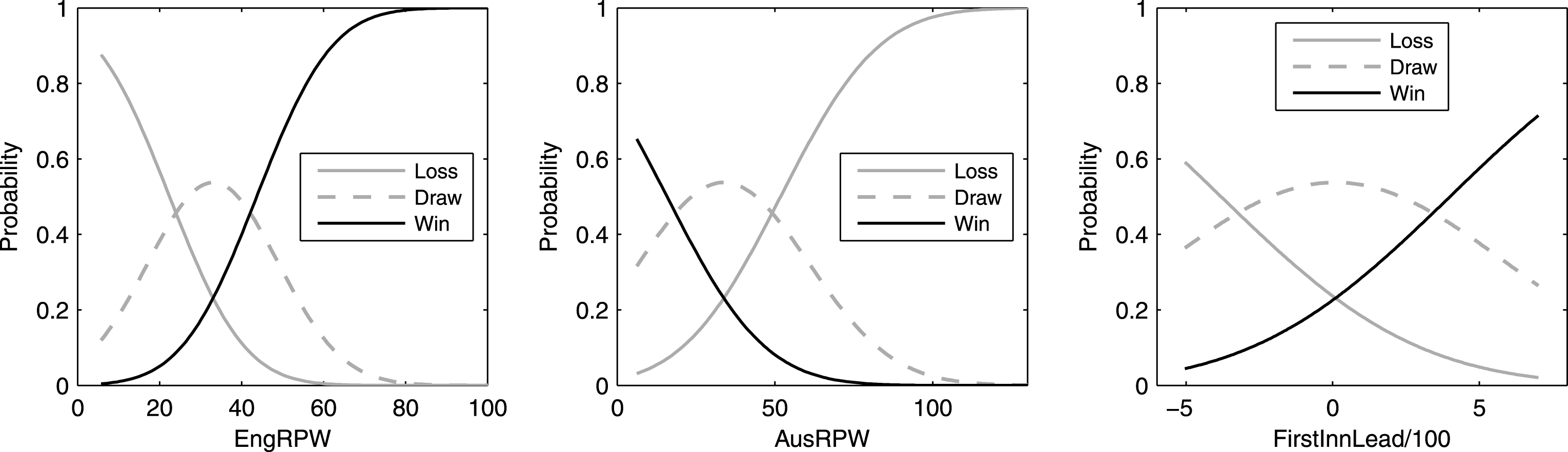
Fig.1
The panels show the fitted probabilities of different Test match outcomes from Model T4.
To further examine the robustness of the results obtained in Table 8, we re-estimate all the models using data for the period 1971-2015. The motivation being that the dynamics of modern Test matches is better captured using data post the introduction of ODI cricket. We observe that the baseline models in Table 9 i.e., Model T7 and Model T8, give results which are quite similar to the baseline models in Table 8. Defensive batting and attacking bowling are significant, while attacking batting and defensive bowling are insignificant. The results on other variables also closely mirror the results from the baseline models, except AusTeamQuality is no longer significant. The results from Model T9 to Model 12 imitate the results from Model T3 to Model T6, respectively, except that the first innings lead becomes strongly significant. However, the variables corresponding to home bias, effect of ODI/T20 on Test matches and location specific strategy of winning the toss and electing to bat remain insignificant. To summarize, we can say that the winning combination of factors/inputs in Test matches have largely remained unchanged over the decades.
In ordinal models, the coefficients by themselves do not give the covariate effects since the link function is not linear. Hence, we calculate the average covariate effect from two selected models and present them in Table 10. In Model T3, EngRPW has the highest positive effect on win probability and an increase in EngRPW by 5 runs changes the probabilities of England’s win, draw and loss by 6.7%, 0.3% and -6.9%, respectively. The highest negative effect on win probability is when match venue is Australia. In this case, England’s probability of win and draw decreases by 8.5% and 1.5%, respectively, and the probability of loss increases by 10.0%. Switching to Model T4, we see that the highest positive and negative effects come from the same variables. Now, an additional five runs per wicket increase (decrease) the probability of win (loss) by 7.0% with no change in probability of draw. Similarly, playing in Australia reduces England’s chances of winning and draw by 11.3% and 1.2%, respectively. Table 10 also displays the covariate effect for AusRPW (an increase of 5 runs), EngWinToss and FirstInnLead (an increase of 50 runs). The covariate effect of these variables can be interpreted similarly and fully conforms to our expectation. We also graphically depict the fitted probabilities of match outcomes from Model T4 (our best fitting model) in Figure 1. The first panel shows that the probability of winning (losing) increases (decreases) with EngRPW and that the probability of a draw is maximized when EngRPW is 33.35. Similarly, the second panel exhibits that chances of winning (losing) decreases (increases) as AusRPW increases with probability of draw maximized at 33.82. The third panel shows that the probability of a win increases as first innings lead increases and the probability of a draw is maximized at 0.05, i.e., with a small first innings lead.
3.2Models and results: ODI
We now turn to ODI matches, which typically result in two outcomes, either loss or win, and is modeled using a binary probit model. The outcome may also be a tie, but it is extremely rare and excluded from this study. Data shows that only two matches between England and Australia have resulted in a tie, once in 1989 and the second in 2005. Similar to Test matches, the ODI outcomes are modeled as a function of match related characteristics presented in Table 6 and the model is estimated using maximum likelihood technique. Interested readers may refer to Johnson and Albert (2000, Chap. 3) or Jeliazkov and Rahman (2012) for a description of binary probit model, estimation techniques and applications.
Table 11
Estimation results for ODI matches from the binary probit model
| model O1 | model O2 | model O3 | model O4 | model O5 | model O6 | |||||||
| coef | t-stat | coef | t-stat | coef | t-stat | coef | t-stat | coef | t-stat | coef | t-stat | |
| Intercept | 1.37 | 0.34 | 1.17 | 0.61 | 4.20† | 1.69 | 3.74 | 1.50 | 2.61 | 1.43 | 2.75 | 1.46 |
| EngRPO | 5.68* | 2.73 | .. | .. | .. | .. | .. | .. | .. | .. | .. | .. |
| EngRPW | 0.23* | 2.60 | 0.16* | 3.85 | 0.16* | 3.85 | 0.16* | 4.02 | 0.15* | 4.19 | 0.16* | 4.19 |
| EngAttackBat | .. | .. | 4.35 | 1.17 | 3.65 | 0.94 | 4.23 | 1.05 | .. | .. | .. | .. |
| AusRPO | –6.41* | –2.76 | .. | .. | .. | .. | .. | .. | .. | .. | .. | .. |
| AusRPW | –0.25* | –2.49 | –0.15* | –4.43 | –0.19* | –3.97 | –0.19* | –3.98 | –0.18* | –4.01 | –0.19* | –3.94 |
| AusAttackBat | .. | .. | –6.42* | –2.15 | –8.93* | –2.21 | –7.64† | –1.87 | .. | .. | .. | .. |
| DiffAttackBat | .. | .. | .. | .. | .. | .. | .. | .. | –6.87* | –2.18 | –6.19* | –1.97 |
| EngTeamQuality | 1.92 | 0.79 | 1.06 | 0.83 | 0.48 | 0.33 | 0.13 | 0.09 | 0.36 | 0.24 | 0.09 | 0.06 |
| AusTeamQuality | 2.88 | 0.70 | –1.25 | –0.71 | –1.46 | –0.67 | –0.89 | –0.41 | –1.93 | –0.89 | –1.05 | –0.49 |
| EngWinToss (w2) | 0.43 | 0.27 | –0.23 | –0.34 | –0.88 | –1.29 | –1.07 | –1.47 | –0.84 | –1.24 | –1.09 | –1.48 |
| EngBatFirst (b2) | –0.22 | –0.18 | –0.63 | –0.88 | –0.74 | –1.01 | –0.95 | –1.30 | –0.60 | –0.86 | –0.89 | –1.24 |
| w2 × b2 | –0.78 | –0.32 | 0.25 | 0.25 | .. | .. | .. | .. | .. | .. | .. | .. |
| VenAus (a2) | 0.54 | 0.46 | –0.31 | –0.51 | –1.26 | –1.57 | –1.27 | –1.60 | –0.79 | –1.25 | –1.03 | –1.50 |
| VenNeutral | –0.19 | –0.14 | –0.63 | –0.64 | .. | .. | .. | .. | .. | .. | .. | .. |
| w2 × b2 × a2 | .. | .. | .. | .. | 1.52 | 1.40 | 1.93 | 1.64 | 1.41 | 1.36 | 1.96† | 1.67 |
| HomeBias | .. | .. | .. | .. | 0.01 | 0.06 | –0.01 | –0.01 | –0.01 | –0.05 | –0.02 | –0.07 |
| Score275 | .. | .. | .. | .. | 0.79 | 0.58 | .. | .. | 0.37 | 0.31 | .. | .. |
| T20I | .. | .. | .. | .. | .. | .. | –0.27 | –0.37 | .. | .. | –0.51 | –0.80 |
| LR (χ2) statistic | 153.27 | 131.36 | 129.52 | 129.31 | 128.33 | 128.87 | ||||||
| McFadden’s R2 | 0.87 | 0.75 | 0.78 | 0.78 | 0.78 | 0.78 | ||||||
| Hit-rate | 95.42 | 94.65 | 95.93 | 94.31 | 95.12 | 95.93 | ||||||
∗ p-value < 0.05, † p-value < 0.10
In Table 11, we present six different models for ODI matches. The first two models i.e., Model O1 and Model O2 are baseline models and utilize information on all the 131 ODI matches. The remaining models (i.e., Model O3 to Model O6) deviate from the baseline models to enable a detailed enquiry similar to Test match models. These models are estimated on 123 matches played either in England or Australia because the variable HomeBias is not well defined for neutral venues. Besides, we restrict ourself to the modern definitions as they are more appropriate for ODI matches. The last three rows of Table 11 represent the LR statistic, McFadden’s R-square and hit-rate. In all the models, the LR statistic is greater than the corresponding critical value and we reject the null hypothesis. McFadden’s R-square and hit-rate are high and indicate good model fit.
We first take a look at the baseline models. Model O1 utilizes traditional measures of batting ability (EngRPO and EngRPW) and bowling ability (AusRPO and AusRPW), along with a host of covariates related to the match. Model O2 replaces EngRPO and AusRPO with their modern definitions, i.e., EngAttackBat and AusAttackBat, respectively. The results suggest that only measures of batting and bowling are important to winning a match. In Model O1, higher EngRPO and EngRPW increases the probability of winning, while higher AusRPO and AusRPW reduces the probability of winning. In Model O2, higher EngRPW raises the probability of winning, but higher AusRPW and AusAttackBat decreases the probability of winning. The finding implies that a combination of attacking/defensive batting and bowling is important for the outcome of a match. This is in contrast to Test matches where only defensive batting and attacking bowling are important to the outcome of a match.
The remaining variables in both the baseline ODI models are all statistically insignificant. Team quality is not important, so it appears that each match outcome is independent of the other. The popular strategy of batting first after winning the toss is also not statistically significant for a match outcome, which is consistent with Cannonier et al. (2015). On the same issue, Bhaskar (2009) finds that batting first after winning the toss reduces the probability of winning for ODI matches played during daytime, but increases the same for day-night ODI matches. Similarly, Dawson et al. (2009) based on an analysis of 649 day-night ODI matches finds that winning the toss and batting increases the probability of winning. We also do not find any statistical evidence of England facing disadvantage while playing in Australia. This is in sharp contrast to what we found for Test matches. Support for home country advantage was reported in De Silva and Swartz (1998), but no such evidence was found in Cannonier et al. (2015). However, the models used in De Silva and Swartz (1998) are not rich in covariates.
Fig.2
The panels show the fitted probability of England winning an ODI match from Model O6.
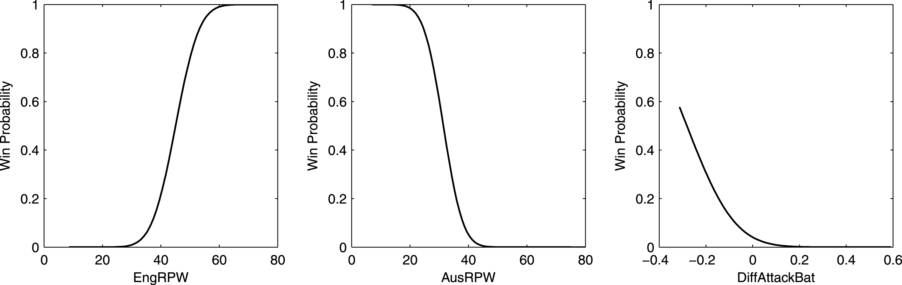
Table 12
Average covariate effects for some selected variables from Model O3 and Model O6
| model o3 | Δ P(y=1) | model o6 | Δ P(y=1) |
| EngRPW (5) | 0.0665 | EngRPW (5) | 0.0660 |
| AusRPW (5) | –0.0786 | AusRPW (5) | –0.0799 |
| AusAttackBat (0.1) | –0.0746 | DiffAttackBat (0.1) | –0.0521 |
Models O3-O6 build on the baseline models and include the variable HomeBias and Score275 or an indicator for post T20 era to capture the impact of T20 on ODI cricket. In addition, we make the interaction term (EngWinToss × EngBatFirst) location specific so as to analyze if the decision to bat first after winning a toss in Australia affects the match outcome differently. We see that in Model O3, the variable EngRPW positively affects the probability of England winning a match, while AusRPW and AusAttackBat negatively affect the winning probability. These results are in conformity with our expectation. Similar to the baseline models, none of the other variables are significant. The coefficient for Score275 and HomeBias are statistically insignificant, implying that there is no evidence of fast paced T20 matches or introduction of neutral umpires affecting the outcome of an England-Australia ODI match. Moreover, there is no significant advantage from the decision to bat first after winning the toss when playing in Australia. We obtain similar results from Model O4, where all the variables are same except that the variable Score275 is replaced by T20I - an indicator variable that takes value 1 if an ODI match is played in the T20 era, 0 otherwise. The coefficients for EngRPW and AusRPW are statistically significant, but AusAttackBat is statistically significant only at 10% level. Once again, we do not find any evidence of T20 matches or home bias affecting an ODI match outcome.
Model O5 and Model O6 are identical to Model O3 and Model O4, respectively; except that we use the difference between AusAttackBat and EngAttackBat (labeled DiffAttackBat in Table 11) instead of including them individually. This specification is encouraged by the fact that while the attacking intent has increased significantly for both teams after the introduction of T20, Australia has become more aggressive than England (see Table 7). The coefficient for DiffAttackBat is negative and statistically significant, which implies that a higher difference reduces England’s probability of winning a match. Similar to previous ODI models, we do not find any significant effect of team quality, electing to bat first after winning the toss, or match venue. Likewise, there is no statistical evidence of T20 or home bias affecting an England-Australia ODI match.
Next, we present the average covariate effect of all significant variables from the two best fitting models in Table 12. In Model O3, when EngRPW (AusRPW) is increased by 5 runs, the probability of England winning the match increases (decreases) by 6.65% (7.86%). An increase in AusAttackBat by 10% (i.e., an increase in proportion of runs accumulated via fours and sixes by 10%) decreases England’s probability of winning by 7.46%. Moving to Model O6, an increase in EngRPW (AusRPW) by 5 runs increases (decreases) the win probability by 6.60% (7.99%). An increase in DiffAttackBat by 10% (i.e., an increase in the difference in proportion of runs accumulated via fours and sixes between Australia and England by 10%) decreases England’s probability of winning by 5.21%. We also pictorially represent the fitted probability of winning from Model O6 in Figure 2. The curves show that the change in win probability is more steep for AusRPW as compared to EngRPW and that probability of win is more positive when DiffAttackBat is negative i.e., proportion of runs in fours and sixes scored by England is higher than that of Australia.
4Discussion
The paper utilizes the production function approach and models the Test and ODI match outcomes between England and Australia as a function of batting, bowling and other variables in order to provide a better understanding of the rivalry between the two cricketing nations. Test match results are ordered (loss, draw or win) and an ordinal probit model is estimated on the 331 Test match data played during 1877-2015. In comparison, ODI match outcomes are dichotomous (loss or win) and studied within a binary probit model based on 131 matches played during 1971-2015. Our model specifications are rich in variables and control for a variety of influences including batting and bowling strategy, team quality, toss outcome, batting order and match venue. Moreover, the models for Test match also include information on first innings lead, length of Test match and weather interruption. We also investigate for potential bias in favor of home team by match officials, the effect of faster format on the longer format of the game and whether they have any influence on the match outcome. Besides, model diagnostic measures indicate that the estimated models have good fit and correctly predict approximately 70% of Test and 95% of ODI match outcomes.
We find that defensive batting and attacking bowling are statistically important for winning Test matches, but a balance of attacking and defensive batting and bowling are vital for ODI match outcomes. Moreover, in Test matches, playing in Australia decreases and first-innings lead substantially increases England’s chances of winning. The differences in importance of batting and bowling inputs can be explained by the fact that while typical innings in Test matches end only when the batting team exhausts all its wickets, innings in ODI can end when the batting team exhausts all the allocated overs. So, a team that scores runs quickly but also loses wickets quickly would be ill-suited to the Test-cricket format, but may be appropriate for ODI as long as it manages to play a decent number of overs and score sufficient runs. It should be noted that while defensive batting and attacking bowling are primary winning strategies in a Test match, the teams playing fixed length (five day) matches may face reverse incentives in a handful of situations. For instance, on the fifth day and fourth innings of the match, if the chasing team has a low target but insufficient time left, it may have an incentive to bat aggressively to prevent the draw, especially if it can afford to lose wickets. Conversely, the bowling team may have an incentive to bowl defensively to waste opponent’s time and drag the match towards a draw. These strategies have been in display by different teams in the past and would definitely occur again in the future.
The differences observed in the winning combination for Test and ODIs should be of interest to the team selection committees as a statistical ratification/rejection of the existing ideas on winning strategies and team composition. In Test matches, it appears that batting average would be a better predictor of player performance as compared to batting strike rate, and hence, must be given more weight in player selection. In ODIs, however, both, batting strike rate and batting average would be important determinants of player performance. Similarly, in Test matches, bowling average would be more important than economy rate, while in ODIs both bowling average and economy rate would be crucial. Note the player attributes that obtain these outcomes may be contingent on the pitch conditions. For example, if the pitches are hard and bouncy, a good team composition would include batsmen who can play fast bowlers and include more fast bowlers than spinners. Besides, adapting to different playing styles is typically a difficult task, and so selection committees may implement format specific team selection (horses for courses) to maximize chances of winning. In fact, some selection committees have been using differential selection policies for a while. For instance, Nathan Lyon (Australia) and Cheteshwar Pujara (India) are mostly selected to play Test cricket, while Eoin Morgan (England) is mostly selected to play ODIs and T20Is. The evidence from our study shows that there is good reason for doing so. The players also stand to gain from this strategy as it will save them from excessive play and burning out, particularly with the enormous amount of cricket (both national and international tournaments) being played throughout a year.
References
1 | Allsopp P.E. and Clarke S.R. , (2004) , Rating teams and analysing outcomes in one-day and test cricket, Journal of the Royal Statistical Society–Series A 167: , 657–667. |
2 | Bairam E.I. , Howells J.M. and Turner G.M. , (1990) , Production functions in cricket: The Australian and New Zealand experience, Applied Economics 22: , 871–879. |
3 | Bhaskar V. , (2009) , Rational Adversaries? Evidence from randomized trial in one day cricket, The Economic Journal 119: , 1–23. |
4 | Bhattacharya M. and Smyth R. , (2003) , The game is not the same: The demand for test match cricket in Australia, Australian Economic Papers 42: , 77–90. |
5 | Borooah V.K. , (2016) , Upstairs and downstairs: the imperfections of cricket’s decision decision review system, Journal of Sports Economics 17: , 64–85. |
6 | Brooks R.D. , Faff R.W. and Sokulsky D. , (2002) , An ordered response model of test cricket performance, Applied Economics 34: , 2353–2365. |
7 | Cannonier C. , Panda B. and Sarangi S. , (2015) , 20-over versus 50-over cricket: Is there a Difference?, Journal of Sports Economics 16: , 760–783. |
8 | Clarke S.R. , (1988) , Dynamic programming in one-day cricket - optimal scoring rates, The Journal of the Operational Research Society 39: , 331–337. |
9 | Crowe S. and Middeldorp J. , (1996) , A comparison of leg before wicket rates between Australian and their visiting teams for test cricket series played in Australia, The Statistician 45 45: , 255–262. |
10 | Dawson P. , Morley B. , Paton D. and Thomas D. , (2009) , To bat or not to bat: An examination of match outcomes in day-night limited overs cricket, Journal of the Operational Research Society 60: , 1786–1793. |
11 | De Silva B.M. and Swartz T. , (1998) , Winning the coin toss and the home team advantage in one-day international cricket matches, New Zealand Statistician 32: , 16–22. |
12 | Demmert H.G. , (1973) , The Economics of Professional Team Sports, Lexington Books, Northampton. |
13 | Forrest D. and Dorsey R. , (2008) , Effect of toss and weather on county cricket championship outcomes, Journal of Sports Sciences 26: , 3–13. |
14 | Jeliazkov I. and Rahman M.A. , (2012) , Binary and ordinal data analysis in economics: Modeling and estimation, in Mathematical Modeling with Multidisciplinary Applications, ed. Yang X. S. , pp. 123–150, John Wiley & Sons Inc., New Jersey. |
15 | Johnson V.E. and Albert J.H. , (2000) , Ordinal Data Modeling, Springer, New York. |
16 | Johnston M.I. , Clarke S.R. and Noble D.H. , (1993) , Assessing player performance in one day cricket using dynamic programming, Asia-Pacific Journal of Operational Research 10: , 45–55. |
17 | Koulis T. , Muthukumarana S. and Briercliffe C.D. , (2014) , A bayesian stochastic model for batting performance evaluation in one-day cricket, Journal of Quantitative Analysis in Sports 10: , 1–13. |
18 | Morley B. and Thomas D. , (2007) , Attendance demand and core support: Evidence from limited overs cricket, Applied Economics 39: , 2085–2097. |
19 | Morley B. and Thomas D. , (2015) , An investigation of home advantage and other factors affecting outcomes in english one-day cricket matches, Journal of Sports Sciences 16: , 760–783 . |
20 | Neale W.C. , (1964) , The peculiar economics of professional sports, Quarterly Journal of Economics 78: , 1–14. |
21 | Perera H. , Gill P. and Swartz T. , (2014) , Declaration guidelines in test cricket, Journal of Quantitative Analysis in Sports 10: , 15–26. |
22 | Ringrose T.J. , (2006) , Neutral umpires and leg before wicket decisions in test cricket, Journal of the Royal Statistical Society–Series A 169: , 903–911. |
23 | Rottenberg S. , (1956) , The baseball player’s labor market, Journal of Political Economy 64: , 242–258. |
24 | Sacheti A. , Gregory-Smith I. and Paton D. , (2014) , “Uncertainty of outcome or strength of teams: An economic analysis of attendance demand for international cricket, Applied Economics 46: , 2034–2046. |
25 | Sacheti A. , Gregory-Smith I. and Paton D. , (2015) , Home bias in officiating: evidence from international cricket, Journal of the Royal Statistical Society–Series A 178: , 741–755. |
26 | Sacheti A. , Paton D. and Gregory-Smith I. , (2016) a, An economic analysis of attendance demand for one day international cricket, Economic Record 92: , 121–136. |
27 | Sacheti A. , Gregory-Smith I. and Paton D. , (2016) b, Managerial decision making under uncertainty: The case of twenty20 cricket, Journal of Sports Economics 17: , 44–63. |
28 | Sargent J. and Bedford A. , (2012) , Using conditional estimates to simulate in-play out-comes in limited overs cricket, Journal of Quantitative Analysis in Sports 8: , 1–20. |
29 | Scarf P. and Akhtar S. , (2011) , An analysis of strategy in the first three innings in test cricket: Declaration and the follow-on, Journal of Operational Research Society 62: , 1931–1940. |
30 | Scarf P. and Shi X. , (2005) , Modelling match outcomes and decision support for setting a final innings target in test cricket, IMA Journal of Mathematics 16: , 161–178. |
31 | Scarf P. , Shi X. and Akhtar S. , (2011) , On the distribution of runs scored and batting strategy in test cricket, Journal of the Royal Statistical Society–Series A 174: , 471–497. |
32 | Schofield J.A. , (1988) , Production functions in sports industry: An empirical analysis of professional cricket, Applied Economics 20: , 177–193. |

