Net best-ball team composition in golf

2.1Net best-ball competitions

Net best-ball competitions are typically based on teams of size m = 2 or teams of size m = 4. And in such competitions, we denote that there are n ≥ 2 teams.

On the jth hole of the course, j = 1, …, 18, the ith player on a given team has a gross score X_ij which represents the number of strokes that it took to hole out. Associated with the ith player on the jth hole is a handicap allowance h_ij = 0, 1, 2 which is related to the quality of the player. The larger the value of h_ij, the weaker the player. Under this framework, the ith player has the resultant net score

The above format is known as stroke play which is the focus of our investigation. When there are only n = 2 teams, then match play competitions are possible. In match play, T_j is calculated as in (2), and the team with the lower value of T_j is said to have won the jth hole. The team with the greatest number of winning holes is the match play winner. Match play typically involves a competition between two teams. In this paper, we focus on the stroke play format.

2.2The current handicapping system

Section 10 of the USGA Handicap System Manual (USGA 2016) provides the intricate details involving the calculation of handicap. However, for ease of exposition, we provide a description of the standard calculation which applies to most golfers.

Consider then a golfer’s most recent 20 rounds of golf where each round is completed on a full 18-hole golf course. The kth round yields the differential D_k which is obtained by

Given a golfer’s scoring record, the golfer’s handicap index is calculated by taking 96% of the average of the 10 best (lowest) differentials and truncating the result to the first decimal place. In Section 2.3, we will see that it is instructive to write the handicap index as

Recognizing that courses are of varying difficulty, the last step for the implementation of handicap involves converting the handicap index to strokes for a particular course. For a course with slope rating S, the course handicap for a golfer with handicap index I is given by C = I × S/113 rounded to the nearest integer.

In the context of net best-ball competitions, the course handicaps C of the players in the tournament are then used to determine the hole-by-hole handicap allowances h_ij in (1). It is at this point where there is some variation in how h_ij is obtained. According to Section 9-4(bii) of the USGA Handicap System Manual (USGA 2016), the recommended way is to first reduce the individual course handicaps C by a factor of 90%, rounding to the nearest integer. An adjustment is then made to the reduced course handicaps where the course handicap for a given golfer is set to the offset between their course handicap and the lowest (best) course handicap in the competition. For example, suppose that the best golfer in the competition has a reduced course handicap C_i1 = 3 and that some other golfer has a reduced course handicap C_i2 = 24. Then the two course handicaps are converted to C_i1 = 3 -3 = 0 and C_i2 = 24 - 3 =21, respectively. Then, we note that the holes on a golf course are assigned a hole handicap according to a stroke allocation table. The table consists of a permutation of the integers 1 to 18 where it is typically thought that increasing numbers correspond to decreasing difficulty of the holes. Denote the hole handicap on the jth hole by HDCP_j. Under the complicated framework described above, h_ij is determined as follows:

Chan, Madras and Puterman (2018) investigated how alternative permutations of HDCP and other innovations affect the fairness of net match play events between two players.

2.3Related literature and ideas

In consultation with the RCGA, Swartz (2009) proposed an alternative handicapping system with the following features:

The key component of the system developed by Swartz (2009) was that it incorporated variability in handicapping. And in the context of net best-ball tournaments, it is clear that amongst two golfers with the same handicap index, a highly variable golfer is more valuable to a team than a consistent golfer. For example, the highly variable golfer will obtain more net birdies which contribute positively to the overall net score of his team. On the other hand, when this highly variable golfer scores net double bogeys, these poor scores are not likely to penalize his team in the best-ball format.

As an alternative to the handicap index/factor, Swartz (2009) defined two statistics that characterize player performance. These statistics are referred to as the mean μˆ and the spread σˆ , and their calculation is analogous to (5). Specifically,

For the purposes of this paper, the spread σˆ in (8) plays a primary role and we record the weights q_i in Table 1. Alternative weights are recorded in Swartz (2009) when a golfer has played fewer than 20 complete rounds. When the spread calculation σˆ falls outside of the interval (1.5,8.0), it is set equal to the corresponding endpoint.

A point that is worth emphasizing is that the calculation of σˆ in (8) is simple and is directly analogous to the calculation of (5) which is part of the current handicapping system. In Section 3, we assume that the values σˆ are available for each golfer in the net best-ball competition. Moreover, the values σˆ are the only values that are needed to form teams according to our proposal. Thus, teams are formed based on the basis of individual performance variability σˆ , and this is the main message of Section 2.

3.1The normality assumption

Whereas the normality of golf scores is frequently assumed in the literature (e.g. Pollock (1977), Scheid (1990), Berry (2010)), these papers assume normality on 18-hole scores. However, in (10), normality is assumed on individual holes. This strong assumption does not strike us as problematic for several reasons. First, the development that follows (10) does not utilize the full distributional properties of the normal. Rather, only the first two moments are used in determining team composition. Second, instead of defining Y_i as the net score of the ith golfer, we could have alternatively defined Y_i as the latent net skill or performance of the ith golfer. Net skill/performance is a continuous variable that is clearly concave and better resembles normality. Although not as clean, such a formulation would have led to the same approach for team composition. We can therefore think of golf scores as a discretized version of skill/performance. But the main point is that the normality argument is provided only as a heuristic for forming teams, and we use actual golf data and simulation to establish that the approach improves upon traditional practice. In Section 4, we supplement the theoretical underpinnings with simulation studies.

4.1Simulation via a theoretical scoring model

In Table 2, we provide probability distributions for 8 fictitious golfers corresponding to their performance on each hole. The distributions are not entirely realistic as we only permit the four net scores of birdie (-1 relative to par), par, bogey (+1 relative to par) and double-bogey (+2 relative to par). However, the probability distributions have been constructed such that each golfer has the same mean net score which is consistent with the desiderata of the handicapping system. The most noteworthy aspect of Table 2 is that the performance of the golfers is variable with increasing standard deviations as we go down the rows of the table. Therefore, golfer 1 is the most consistent and golfer 8 is the most variable.

Imagine that these 8 golfers are competing in teams of size m = 2. Therefore, the number of possible tournament constructions is (28)(26)(24)/4!=105 . Consider one such tournament construction. For each team, we first generate 18 holes for each golfer in the pair according to their probability distributions in Table 2. We then determine the team’s aggregate net best-ball score T according to (3). For this particular round of 18 holes and for the particular tournament construction, we determine the finishing order of the four teams. We repeat the simulation procedure for 1,000 tournaments to obtain frequency tables for the finishing positions. Note that if a tie exists for a particular round, we randomly break ties.

According to our proposed team composition developed in Section 3, the optimal tournament construction in terms of fairness is 1&8, 2&7, 3&6 and 4&5. We denote this tournament construction as WCS (an acronym based on the authors’ surnames). We are interested in how WCS performs compared to the other 104 potential tournament constructions. Table 3 provides the percentage of time in the WCS simulation corresponding to the four finishing positions for each of the four teams. If the competition were completely fair, the table entries would all be equal (i.e., 25.0%). For WCS, we observe that Team 1&8 is clearly the strongest team finishing in the top two positions nearly 66% of the time.

However, whether WCS is meritorious can only be determined in the context of the other potential tournament constructions. And each tournament construction has a corresponding Table 3 resulting from the simulation procedure. For each tournament construction, it is natural to assess fairness via the Chi-Square test statistic

Table 4 lists the best performing and worst performing tournament constructions based on the Chi-Square test statistic (12). Although none of the team constructions are fair (i.e., they all have p-values that are statistically significant), we observe that our proposed team formation WCS is the best possible tournament construction. It is the best construction that can be achieved given the characteristics of the 8 golfers and the rules of net best-ball tournaments. We also note that the best five tournament constructions are similar in the sense that golfers with high variability are paired with ones with low variability.

4.2Simulation via actual golf scores

This simulation study is based on a dataset obtained from Coloniale Golf Club in Beaumont, Alberta collected over the years 1996 through 1999.

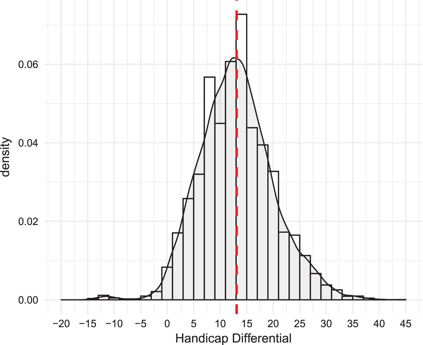
After restricting scores to male golfers who have played at least 40 rounds, we are left with a dataset consisting of 10,470 rounds collected on 80 golfers. Therefore, the average number of rounds played per golfer in the restricted dataset is approximately 131. In Figure 1, we provide a histogram and density plot of the handicap differentials corresponding to the 10,470 rounds. The mean handicap differential is approximately 13 and is marked by the dashed vertical line. The data correspond to a large pool of golfers with varying skill levels. It should therefore have the required generality for testing our proposed method of team formation in net best-ball tournaments.

Fig.1

Histogram and density plot of the handicap differentials for the Coloniale dataset.

Our simulation procedure is based on a resampling scheme. In this exercise, suppose that we investigate a particular team construction heuristic where we form n = 20 teams of size m = 4. For each golfer, our first step involves randomly selecting 20 of his rounds of golf. These rounds will form his 20 differentials from which his handicap index I in (5) and his spread statistic σˆ in (8) can be calculated. These two statistics are sufficient for determining all of the common methods of team composition including our proposed method. Therefore, based on the particular team construction heuristic, the 20 teams of four players are identified. For each of these 80 golfers, we next generate one of their remaining rounds of golf for which we have hole-by-hole scores. In golf, detailed hole-by-hole data is rare and is a feature of the Coloniale dataset. Using the generated round of golf for each of the 80 golfers, each team’s aggregate net best-ball score T can be calculated according to (3), and we obtain the finishing order of the 20 teams composed by the particular team construction heuristic. This resampling procedure is repeated over 40,000 hypothetical tournaments. Frequency tables are obtained as in Table 3 where finishing order corresponds to the rows and team compositions correspond to the columns. In this simulation exercise we therefore have matrices of dimension 20 × 20.

We now compare two common team constructions against our proposed method WCS and a variation of WCS. Recall from Section 3 that our method of team formation first ranks golfers according to σˆ , and then pairs golfers 1&80, 2&79, and so on. Then, these 40 pairs are ranked according to σˆi12+σˆi22 where i₁ and i₂ are in the same pair. We then pair the pairs as before with high values of σˆi12+σˆi22 matched with low values. This algorithm determines the 4-man teams.

We refer to the most common method of team formation as “High-Low” where High-Low is very similar in construction to WCS. The only difference is that orderings are based on the handicap index I in (5) rather than spread statistic σˆ in (8). The High-Low heuristic is that strong golfers are matched with weak golfers in the first pairing, and then strong teams (based on cumulative handicap indices) are matched with weak teams in the subsequent pairing.

We refer to the third method of team formation as “Zigzag” which is less common than High-Low. Pavlikov, Hearn and Uryasev (2014) provide an illustrative example of Zigzag. For simplicity, consider the formation of 16 golfers into four teams of four players as shown in Table 5. For example, Team 1 consists of golfers 1, 8, 9 and 16. The intuition behind Zigzag is that the summation of handicap indices should be nearly constant across teams.

The fourth method which we refer to as “WCS_Z” is a “Zigzag” variation of WCS. In WCS_Z, we carry out the Zigzag team formation procedure but instead of using handicap indices, we use the spread statistic σˆ .

In Table 6, we provide the results of the comparison using the simulated frequency tables based on High-Low, Zigzag, WCS and WCS_Z. In this exercise, the Chi-Square statistic (12) is used to assess the four methods of team formation where the summations in (12) extend over the 20 × 20 cells and E_ij = 2, 000. We observe that WCS_Z outperforms the other three methods in terms of giving the lowest Chi-Square statistic. The High-Low method is clearly the worst of the three methods in terms of fairness.

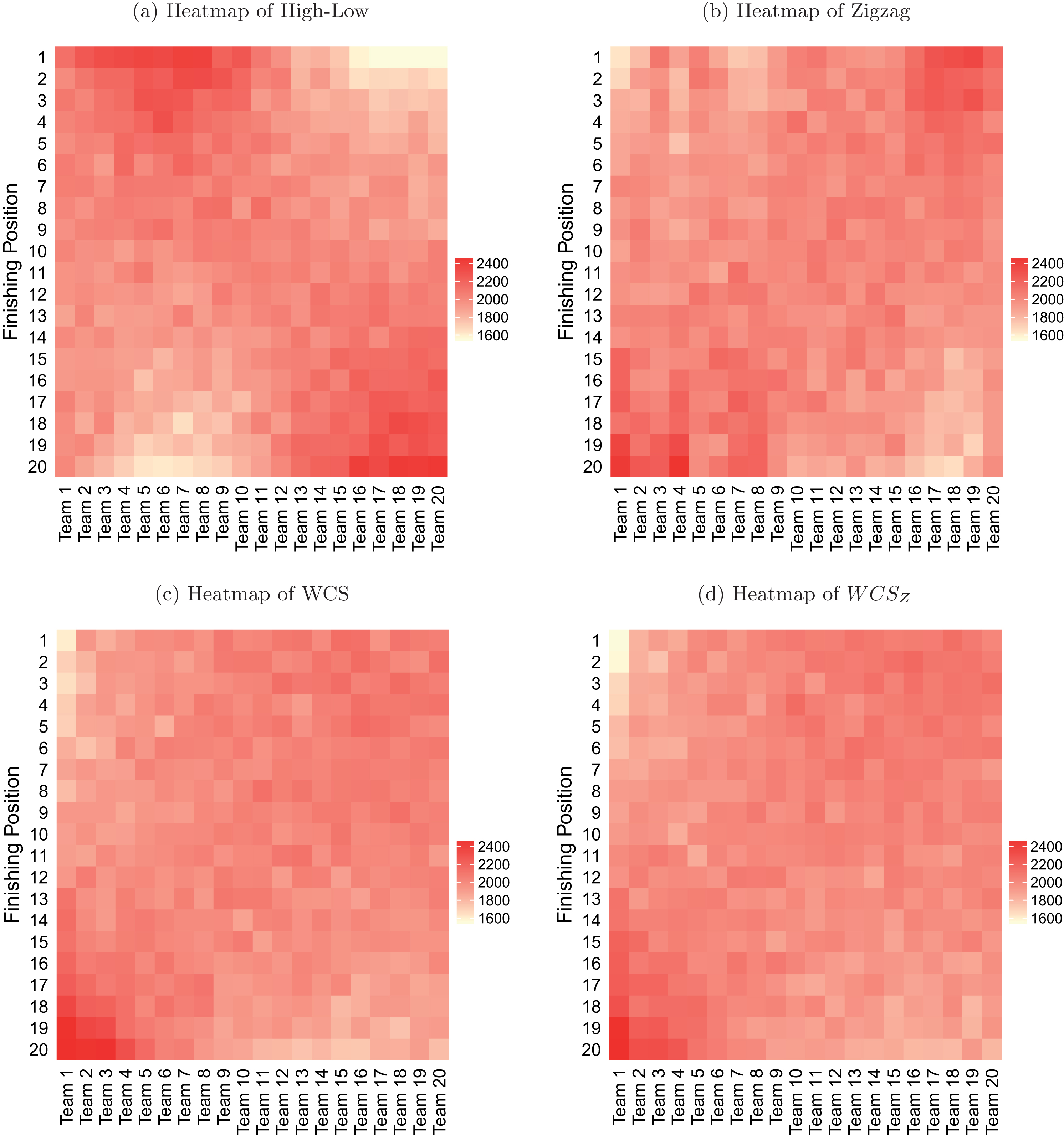
Another way of assessing the four methods is via heatmaps. In Figure 2, we produce heatmaps corresponding to the simulated frequency tables based on High-Low, Zigzag, WCS and WCS_Z. It is evident that the new approaches (WCS and WCS_Z) have more constant coloring; this indicates that they are fairer methods of team composition than both High-Low and Zigzag.

Fig.2

Heatmaps of the frequency tables produced by High-Low, Zigzag, WCS and WCS_Z.

References

1 | Benincasa,G. , Pavlikov,K. and Hearn,D. , (2017) , Algorithms and software for the golf director problem. Available at www.optimization-online.org/DB FILE/2017/10/6299.pdf (Accessed: 23 July 2018). |
2 | Berry,S.M. , (2010) , Is Tiger Woods a winner? In Mathematics and Sports, Dolciani Mathematical Expositions #43, J.A. Gallian, editor, Mathematics Association of America: Washington, 157–168. |
3 | Bingham,D.R. and Swartz,T.B. , (2000) , Equitable handicapping in golf, The American Statistician, 54: (3), 170–177. |
4 | Chan,T. , Madras,D. and Puterman,M. , (2018) , Improving fairness in match play golf through enhanced handicap allocation, Journal of Sports Analytics, Prepress, 1–12. |
5 | Golf Canada, 2016, Golf Canada Handicap Manual. Available at http://golfcanada.ca/app/uploads/2016/02/2016-Handicap-Manual-6x9-ENG-FA-web.pdf (Accessed: 21 August 2017). |
6 | Grasman,S.E. and Thomas,B.W. , (2013) , Scrambled experts: Team handicaps and win probabilities for golf scrambles, Journal of Quantitative Analysis in Sports, 9: , 217–227. |
7 | Hurley,W.J. and Sauerbrei,T. , (2015) , Handicapping net best-ball team matches in golf, Chance, 28: , 26–30. |
8 | Kupper,L.L. , Hearne,L.B. , Martin,S.L. and Griffin,J.M. , (2001) , Is the USGA golf handicap system equitable? Chance, 14: (1), 30–35. |
9 | Nadarajah,S. and Kotz,S. , (2008) , Exact distribution of the max/min of two gaussian random variables, IEEE Transactions on Very Large Scale Integration (VLSI) Systems, 16: (2), 210–212. |
10 | Pavlikov,K. , Hearn,D. and Uryasev,S. , (2014) , The golf director problem: Forming teams for club golf competitions. In Social Networks and the Economics of Sports, Pardalos,P.M. and Zamaraev,V. , editors, Springer International Publishing: Switzerland, 157–170. |
11 | Pollock,S.M. , (1974) , A model for the evaluation of golf handicapping, Operations Research, 22: (5), 1040–1050. |
12 | Pollock,S.M. , (1977) , A model of the USGA handicap system and fairness of medal and match play. In Optimal Strategies in Sports, Ladany,S.P. and Machol,R.E. , editors, North Holland: Amsterdam, 141–150. |
13 | Scheid,F.J. , (1977) , An evaluation of the handicap system of the United States Golf Association. In Optimal Strategies in Sports, Ladany,S.P. and Machol,R.E. , editors, North Holland: Amsterdam, 151–155. |
14 | Scheid,F.J. , (1990) , On the normality and independence of golf scores, with various applications. In Proceedings of the First World Scientific Congress of Golf, Cochran,A.J. , editors, E & FN Spon: London, 147–152. |
15 | Siegbahn,P. and Hearn,D. , (2010) , A study of fairness in fourball golf competition. In Optimal Strategies in Sports Economics and Management, Butenko,S. , Gil-Lafuente,J. and Pardalos,P.M. , editors, Springer-Verlag:Heidelberg, 143–170. |
16 | Swartz,T.B. , (2009) , A new handicapping system for golf, Journal of Quantitative Analysis in Sports, 5: (2), Article 9. |
17 | USGA 2016, USGA Handicap System Manual. Available at http://www.usga.org/Handicapping/handicap-manual.html#!rule-14367 (Accessed: 21 August 2017). |
18 | Yun,H. , 2011a History of handicapping, part I: Roots of the system. Available at http://www.usga.org/articles/2011/10/history-of-handicapping-part-i-roots-of-the-system-21474843620.html (Accessed: 21 August 2017). |
19 | Yun,H. , 2011b History of handicapping, part II: Increasing demand. Available at http://www.usga.org/content/usga/home-page/articles/2011/10/history-of-handicapping-part-ii-increasing-demand-21474843658.html (Accessed: 21 August 2017). |
20 | Yun,H. , 2011c History of handicapping, part III: USGA leads the way. Available at http://www.usga.org/content/usga/home-page/articles/2011/10/history-of-handicapping-part-iii-usga-leads-the-way-21474843686.html (Accessed: 21 August 2017). |
21 | Yun,H. , 2011d History of handicapping, part IV: The rise of the slope system. Available at http://www.usga.org/content/usga/home-page/articles/2011/10/history-of-handicapping-part-iv-the-rise-of-the-slope-system-21474843751.html (Accessed: 21 August 2017). |