
What was lost? A causal estimate of fourth down behavior in the National Football League
Abstract
In part driven by academic research, perception in the sports analytics community asserts that coaches in the National Football League are too conservative on fourth down. Using 13 years of data, we confirm this premise and quantify the unobserved benefit that teams have missed out on by not utilizing a better fourth down strategy. Formally, teams that went for it are paired to those who did not go for it via a nearest neighbor matching algorithm. Within the matched cohort, we estimate the additional number of wins that each NFL team would have added by implementing a basic but more aggressive fourth down strategy. We find that, on average, a better strategy would have been worth roughly an extra 0.4 wins per year for each team. Our results better inform decision-making in a high-stakes environment where standard statistical tools, while informative, have possibly been confounded by extraneous factors.
1Introduction
Past research has linked National Football League (NFL) coaches and team personnel to suboptimal decision-making (Romer, 2006; Kovash and Levitt, 2009; Massey and Thaler, 2013). For example, Massey and Thaler (2013) assert that NFL coaches are not among the group of elite managers who are capable of complex analysis required to calculate probabilities and act impartially.
One important aspect of football that requires the frequent input of the head coach is what to do on fourth down plays. Offensive teams on fourth downs can either go for it (via a rush or a pass attempt) or kick it (via a field goal or a punt). This decision is typically made by the team’s head coach, who, from the sideline, makes the choice to go for it or kick within a matter of seconds. Play selection is informed by, among other factors, the distance needed to obtain a first down, location of the ball on the field, each team’s ability, the game’s score, and how much time remains in the game.
In his seminal work, Romer (2006) suggested that NFL coaches were too passive on fourth downs, and instead were punting and kicking field goals too often. This work received national attention (Lewis, 2006) and inspired the development of a public-facing tool from The New York Times to provide recommended fourth down decisions in real-time (Burke et al., 2013; Causey et al., 2015). However, it’s been more than a decade since Romer’s work, and despite the publicity, the rate of fourth down attempts has not increased over time (see Section 2).
The primary goal of this manuscript is to estimate the potential benefit that teams have missed out on by not being more aggressive on fourth downs. Romer (2006), for example, proposed that a proper fourth down strategy would be worth one extra win every three years. However, this estimate was not the primary objective of his work, and his findings are estimated without the consideration of several factors influencing fourth down success rates.
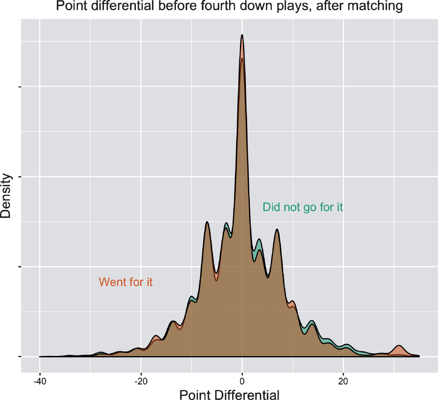
For our purposes, it will be critical to account for as many of the game and play characteristics that weigh on coaches’ minds as possible. As an example, Figure 1 shows density curves of point differential for all fourth down plays between 2004 and 2016, relative to the offensive team, and split for teams that did and did not go for it. The curve for teams that did not go for it is symmetric, centered at 0 (a tie game) with various peaks to the left and right, including point differentials of ±7 and ±14. Among teams that went for it, the modal point differential is -7 points. The curve has a greater density with negative point differentials, implying that teams that went for it were usually trailing. Given that trailing teams are, in general, less talented, using the success rate of these teams as representative of all teams would potentially underestimate the chance of converting that more talented teams would have. Of course, there are several additional components other than the games’ score that likewise impact how coaches make fourth down decisions.
Fig.1
Density curves showing the distributions of point differential (relative to the offensive team) among teams that went for it on fourth down and teams that did not. Shown are all fourth down plays from the 2004 through 2016 seasons (37,103 total plays) of the National Football League, using regular season games only.

We use matched methods with finite population propensity scores (Imbens and Rubin, 2015) to help account for point differential and other factors impacting fourth down decisions. Formally, we link plays where a team kicked on fourth down, defined as our control, to a play where a team went for it, defined as our treatment, using a sample of plays where, according to a basic statistical model, teams should have gone for it. Plays are matched based on their yards to go for a first down, the play with the nearest predicted probability of going for it, closest in-game win probability, and most similar game time. Within the matched cohort of plays, we estimate the observed change in win probability after each fourth down play. Using these outcomes, we aggregate across each franchise to approximate the number of wins that each team would have added over the past 13 seasons if it had been more aggressive on fourth down. For nearly all teams, there is evidence that a basic but aggressive fourth down strategy would have increased the teams’ win total. On average, we estimate that the strategy would have been worth about 0.4 wins per year, with some evidence suggesting that certain teams would benefit more than others.
Our paper is outlined as follows. Section 2 in Sports reviews previous fourth down studies. Section 3 introduces our notation, describes the data source and data cleaning, and reviews the components of our matching algorithm. Section 4 implements the matching, with results described in Section 5. Finally, we discuss potential explanations for our findings in Section 6, as well as possible future extensions.
2Fourth Down Decision Making in the NFL
We begin by reviewing past research into fourth down decision-making in the NFL.
Carter and Machol (1978) were among the first to use statistics to judge fourth down strategies, using an expected points framework to compare going for it to punting and kicking field goals. Albeit in a substantially different time, the authors found that teams kicked too many field goals. With more recent data, Romer (2006) estimated a smooth function of expected points for the offensive team on every yard line of the field when teams had one yard to go for a first down, and subtracted the expected points for the defensive team based on where they would receive the ball were the offensive team to have kicked. Using dynamic programming, Romer found that teams were generally not aggressive enough on fourth down. Romer did not account for team ability, game situation, or other variables linked to fourth down success, and only fourth down attempts with one yard to go were considered. Altogether, Romer estimated that a more aggressive fourth down strategy would be worth about a third of a win per year.
Burke and Quealy (2013) expanded Romer’s study by testing not only one yard to go scenarios, but every yards to go distance and line of scrimmage throughout the field. Similar to Romer, most of Burke and Quealy’s findings were driven by expected point calculations. The authors used their findings to develop a fourth down strategy, shown in the Appendix (Figure 8), which identifies when teams should ‘go for it’, ‘punt’ or kick a ‘field goal,’ depending on yards to go and field location (Burke and Quealy, 2013). Not surprisingly, the fourth down strategy endorsed by Burke and Quealy (2013) differed significantly from the decisions that coaches most often made (see Figure 8). These authors also helped create a social media interface for The New York Times, termed the ‘4th Down Bot,’ that identified recommended choices for teams in real time. Most recently, Causey et al. (2015) expanded this project prior to the 2015 season, assessing fourth down choices using a cross-validated logistic regression model of win probability.
Despite the attention, there is no known evidence that coaches’ decisions were modified after Romer (2006). Figure 2 shows the proportion of times that offensive teams with fourth down attempts in the ‘go for it’ range of the 4th Down Bot actually went for it, using all regular season games from 2004 through 2016.
Fig.2
Proportion of times that teams with fourth down attempts within the ‘go for it’ range of The New York Times’ 4th Down Bot actually went for it, per season. There is no evidence that teams have increased their rates of going for it over time.
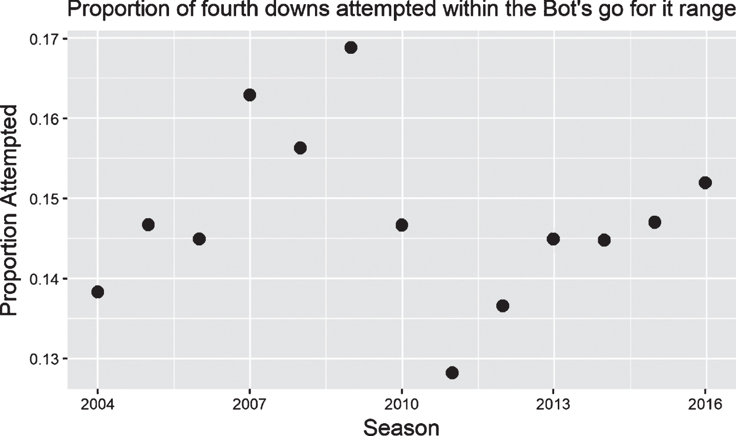
Since the 2004 season, the rate of fourth downs has fluctuated between 12 percent and 17 percent, with no obvious change over time.
There are a few explanations for the perceived conservative behavior of NFL coaches. One oft-cited justification is that coaches are risk-adverse (Urschel and Zhuang, 2011). More often than not, going for it is a riskier move, as the reward for a successful conversion is offset by the setback that comes from a failed attempt. In the quote prefacing this manuscript, former Pittsburgh Steelers Coach Bill Cowher mentions “costing” a team a football game when a fourth down attempt falls short. Such failures may be blamed on the coach, whereas the choice to kick generally yields no such ridicule from team personnel and fans. In fact, for a coach, while kicking may not maximize his teams’ chance of winning a given game, it could actually maximize his chance of keeping a job. Indeed, a version of this theory was confirmed empirically by Owens and Roach (2017) in college football, with the authors finding that coaches grew more conservative on fourth downs as they became more likely to be fired.
A related explanation for coaches’ behavior is loss-aversion (Tversky and Kahneman, 1991). Moskowitz and Wertheim (2012), for example, attribute wrong fourth down decisions to a fear of losing. The authors quote former baseball manager Sparky Anderson: “Losing hurts twice as bad as winning feels good." In the case of NFL coaches, the fear of ridicule and criticism after a loss could impair decision-making under pressure. As a result, coaches may act in ways that avoid obvious explanations for losing.
Apart from Romer’s estimate, we are unaware of any attempt to quantify exactly how an aggressive fourth down strategy could benefit a team. In the sections that follow, we use matched methods to estimate this missed benefit.
3Framework: the Rubin Causal Model
Ideally, prior to any fourth down decision, a coach is aware of the play outcomes of both a conversion attempt and a kick. Of course, this optimal scenario is not possible, as we only get to observe the outcome under one of the two paths (whichever one is chosen by the coach). Statistically, this conundrum is known as the fundamental problem of causal inference, as we are missing the fourth down outcome that isn’t observed (Rubin, 1974).
The best design for making inference about the causal effects of aggressive fourth down decision-making would be to use randomized experiments (Cochran and Chambers, 1965). Randomized designs are admired for many reasons: they are, in expectation, unbiased in the distribution of covariates between treatment and control groups, and systematically favoring treatment or control is impossible because the researcher does not have access to any knowledge of the outcome (Rubin, 1974). However, in the high-stakes environment of the National Football League, randomized designs that would make some teams go for it and others not go for it are infeasible. Fortunately, it is possible to mimic some of the advantages of a randomized experiment through causal inference and the Rubin Causal Model (RCM).
We start by identifying a group of fourth down plays where it is reasonable to argue that teams should go for it. For simplicity, we use recommendations of the two-dimensional 4th Down Bot (see Figure 8 in the Appendix), which depend on both yards to go for a first down and the offensive team’s distance from its own end zone. Let Y be our outcome, defined as the change in offensive team’s win probability from before each play to after each play, and let W be a treatment indicator for whether or not a team went for it (defined as a rush or pass attempt) in this range of plays. The potential outcome of each play, Y (W), reflects the change in win probability that would have been observed under each of the two treatments, going for it, Y (W = 1) = Y (1), and not going for it, Y (W = 0) = Y (0). The win probability models that estimate these potential outcomes are described in Section 3.4.
The RCM assumes two conditions, termed the stable unit treatment value assumption (SUTVA), with respect to W. First, the potential outcome for one observation does not vary based on the treatments assigned to other subjects. In our example, changes in win probability after one team’s fourth down attempt are unlikely to be linked to another team’s fourth down choice. A second assumption of SUTVA is that there is no hidden variation of treatment. In football, the decision to go for it is made prior to any play and reflects a choice consistent betweenall teams.
Under SUTVA, we next explain the assignment mechanism of the RCM. For every play i there is an observed outcome,
To date, the majority of 4th down literature has focused on how, in certain game settings, E [Yi (Wi = 1) - Yi (Wi = 0)] >0. That is, in expectation, going for it is better than not going for it. Alternatively, our primary interest lies in what would have happened to the control units – the teams that did not go for it – had they instead gone for it. This estimand is termed the average treatment effect on the control (ATC). For each play, the unit level causal estimand, ATCi, reflects the difference in potential outcomes between going for it (outcome
(1)
More generally, Equation (2) reflects the overall average difference in outcomes between our treatment and control groups among all plays in the control group where a team did not go for it. Here,
(2)
To estimate franchise specific effects, consider TTCf, the total treatment effect on the control for franchise f, where
(3)
This estimand represents the total increase in win probability for franchise f were it to have gone for it on all of its plays in the 4th Down Bot’s recommended range. Here, I (Fi = f) is an indicator for whether or not the offensive team in question corresponds to franchise f.
Two assumptions are required to estimate (1) - (3). First, we assume positivity, that Pr (Wi = 0|Xi) >0 and Pr (Wi = 1|Xi) >0 for all i. This requires teams to have a non-zero chance of both going for it and not going for it on a given fourth down play. Given the rules of football, as well as our matching implementation in Section 3.3, this assumption seems reasonable. Next, let X be a set of play and game characteristics that are associated with W and Y. Our second assumption is that of ignorability, which states that Pr (W|X, Y (0) , Y (1)) = Pr (W|X) for all W, X, Y (0), and Y (1). In other words, there are no other variables besides those in X linking the choice to go for it with fourth down potential outcomes. We note that this assumption is not testable, and requires subject level expertise with respect to choosing variables for X.
Under the assumptions above, the decision to go for it is deemed strongly ignorable, implying that the joint distribution of Y (0) and Y (1) is conditionally independent of W, and solely on the covariate values, X,
Under this assumption, Yi (1) - Yi (0) is an unbiased estimate of the causal effect of going for it on play i.
Because there are a number of covariates in X that dictate a team’s choice to go for it, it would be impossible to match observations with identical X’s. Instead, the use of the propensity score, e (x), summarized in Section 3.2, allows us to use a similar strongly ignorable assumption, such that
3.1Data
We obtained play and game level data from ArmchairAnalysis . com (AA) for all NFL seasons from 2004 through 2016.2 We match only within the subgroup of regular season plays where the 4th Down Bot recommends that a team should have gone for it, leaving n= 13,172 fourth downs, on which teams failed to go for it 9,348 times (71.0%).
AA’s data contain several play and game characteristics that may be linked to fourth down decision making. In addition, we obtained pass and rush team-level ratings from FootballOutsiders . com for each team’s offensive and defensive units in each season. These ratings measure the team’s offensive and defensive strengths as a percentage of the league average, and are calculated using yards gained, points scored, and other metrics.3
Our list of variables is shown in Table 1. Unless otherwise noted, the variables come from AA.
Table 1
Covariates and Descriptions. All variables were obtained from Armchair Analysis unless otherwise indicated
| Covariate | Description |
| yfog | Yards from own goal |
| ytg | Yards to go for a first down |
| pointdiff | Difference in offensive and defensive teams’ scores: |
| M4 (-17 or less), M3 (-16 to -9), M2 (-8 to -4), M1 (-3 to -1), T (0), | |
| P1 (1 to 3), P2 (4 to 8), P3 (9 to 16), P4 (17 or more) | |
| time | Elapsed time in minutes |
| condcat | Weather category: Precipitation, Dry, or Dome |
| temp | Temperature at kickoff (in degrees Fahrenheit) |
| humd | Percent humidity |
| wspd | Windspeed at kickoff (in miles per hour) |
| sprv | Las Vegas point spread |
| ou | Las Vegas over-under (total points) |
| wp | Pre-snap win probability for the offensive team, averaged |
| between two win probability models | |
| Home | Factor variable for home or away |
| wk | Week of the season |
| OR . pass | Offensive team’s pass offense rating (from Football Outsiders) |
| OR . rush | Offensive team’s rush offense rating (from Football Outsiders) |
| DR . pass | Defensive team’s pass defense rating (from Football Outsiders) |
| DR . rush | Defensive team’s rush offense rating (from Football Outsiders) |
As one data cleaning note, we removed all fourth down plays on which a penalty occurred, as we were unable to decipher the corresponding fourth down decision (to go for it or to kick) in the AA data. Additionally, wind speed, temperature and humidity variables were not recorded for most games played inside a dome. Where this information was missing, we imputed the wind speed as 0 miles per hour, the temperature as 70 degrees Fahrenheit, and humidity as 60%.
Although we cannot share the data due to Armchair Analysis restrictions,4 our entire analysis plan is available on Github in a public repository, found at https://github.com/statsbylopez/nfl-fourth-down. This includes.RData files for both win probability models, as well as code for each of (i) data wrangling and win probability calibrations, (ii) our matching algorithm and its analysis, and (iii) results.
3.2Propensity Score Model
Our propensity score model estimates e (X) = P (W|X), the probability of a team going for it given the play and game characteristics of each fourth down attempt. As explained in Section 3, due to the large number of covariates influencing the decision to go for it, e (X) helps appease the strongly ignorable assignment assumption. We used a multiple logistic regression model with spline terms to estimate e (X), using all covariates defined in Table 1. The ultimate goal of estimating e (X) is to balance the variables in X between the teams that went for it and the teams that did not. Stuart (2010) favors more comprehensive models at the expense of simpler ones, as the penalty for including a variable with little association to W is, generally, only a slight increase in variance. The full list of interaction terms (chosen using the authors’ familiarity with football) and spline knots used in the propensity score model can be found in Table 3 of Covariates in the Appendix.
In order to ensure that we have equivalent cohorts, we filter out all observations where the propensity score distributions do not overlap, as extrapolating to these plays would require making unjustifiable assumptions. Less formally, there are fourth down plays where a team would almost never go for it (i.e. e (x) ≈0), and identifying a play where a team did go for it in such a situation may be impossible. Similarly, there may be situations where all teams would go for it (i.e. e (x) ≈1). We filter this range by calculating the maximum and minimum values of e (x) for each of the treatment and control groups, removing all observations with e (x) greater than the maximum in the control group and less than the minimum in the treatment group. This range for e (x) represents a common support interval (Dehejia and Wahba, 1999), giving us a sample size of n = 12, 250 fourth down plays (of which teams failed to go for it 8,812 times, or 72%). The propensity score model is then refit on this sample.
3.3Matching
We used a 1:1 nearest neighbor matching algorithm with replacement via the Matching package in R (Sekhon, 2008), pairing teams that did not go for it to those that did. One-to-one matching (as opposed to one-to-two or one-to-k) appeared to be our only reasonable option given the relative lack of number of teams that went for it in certain situations. Matching was done with respect to four play characteristics: logit (e (X)) (the logit transform of the propensity score), logit (wp) (the logit transform of the offensive team’s pre-snap win probability), ytg (yards to go), and time, the number of minutes remaining in the game. For logit (e (X)) and logit (wp), we use a caliper of.5, ensuring that all matches are within one half of their respective standard deviations. Pre-snap win probability is included as a matching variable given that the range of possible changes in each play’s wp are inherently linked to its’ pre-snap wp. We match with caliper 0 on ytg (e.g., 4th-and-1 plays are only matched to other 4th-and-1 plays, etc). Finally, we use a caliper of 7.5 minutes for time to avoid matching plays in the beginning of the game to plays at the end of the game. Each team that did not go for it was matched to exactly one team that did go for it.5
One key to causal inference methods is to design the study without access to the outcomes. This is in an effort to mimic a randomized experiment, where the observed outcomes are not known until the entire study has been conducted. Thus, we conducted all of the aforementioned methods without viewing our outcomes.
3.4Outcome
Our outcome is Y = Δwp, the change in offensive team’s win probability from before to after each fourth down play. Win probabilities for each play were averaged using two known, calibrated models. The first win probability model is a replication of the random forest algorithm constructed by Lock and Nettleton (2014). The second is a generalized additive model adapted from Horowitz (2016). Both models are constructed using the predictor variables listed in Table 2. For a more in depth description of the models, including a calibration test for each, see Appendix A.1.
Table 2
Descriptions of variables used in models of win probability (wp)
| Variable | Description |
| Down | The current down (1st, 2nd, 3rd or 4th) |
| Score | Difference in offensive and defensive teams’ score |
| Seconds | Number of seconds remaining in game |
| ScoreLeverage |
|
| sprv | Las Vegas pre-game point spread |
| timo | Time outs remaining for the offensive team |
| timd | Time outs remaining for the defensive team |
| TotalPoints | Total points scored in the game |
| yfog | Yards from own goal |
| ytg | Yards to go for a first down |
4Matching Implementation
Our original data consisted of 37,103 4th down plays between the 2004 and 2016 seasons. Filtering plays within the ‘go for it’ range of the 4th Down Bot yielded 13,172 plays, of which teams failed to go for it 9,348 times. Next, after dropping plays outside a common support interval, we retained 12,250 fourth down plays (of which teams kicked 8,812 times). Finally, after matching plays based on the methods described in section 3.3, we retained 7,698 pairs of plays. Each pair included one play where a team did not go for it, as well as a corresponding match where a different team did go for it.
We provide an example of the matching algorithm for clarity. According to the 4th Down Bot, one play where a team did not go for it but should have occurred during week 14 of the 2013 season, where the Atlanta Falcons had a 4th-and-2, 65 yards from their own goal, 5 minutes into a tied game against the Green Bay Packers. Atlanta chose to punt, giving Green Bay the ball at its own 10-yard line. Overall, the punt yielded a Y = Δwp = -2.4% for Atlanta. This Atlanta play was paired to a similar situation where a team did go for it in a game between the New England Patriots and New Orleans Saints during week 11 of the 2005 season. New England faced a 4th-and-2, 68 yards from its own goal, 10 minutes into a tied game, and successfully converted a four-yard pass, resulting in a Y = Δwp = 8.5%. Via Equation (1), this play-level ATCi is an estimated 8.5 - (-2.4) =10.9%.
Matching success across all plays in the matched cohort is best measured by comparing the distributions of X between teams that went for it and those that did not go for it. As an example, Figure 3 shows density curves of point differential within this subset of plays. In Figure 3, the point differential of teams that went for it is a near perfect overlap with their corresponding matches, standing in stark contrast to Figure 1. At least with respect to point differential, our matching algorithm has successfully found like subgroups of plays.
Fig.3
Density curves showing the distributions of point differential among teams that went for it on fourth down and teams that did not. Shown are all 4th-down plays from the 2004 through 2016 seasons included in our matched analysis (7,698 pairs of plays).
To simplify the assessment of covariates’ balance for all X in Table 1, we use standardized bias, SBx, where for any variable x ∈ X,
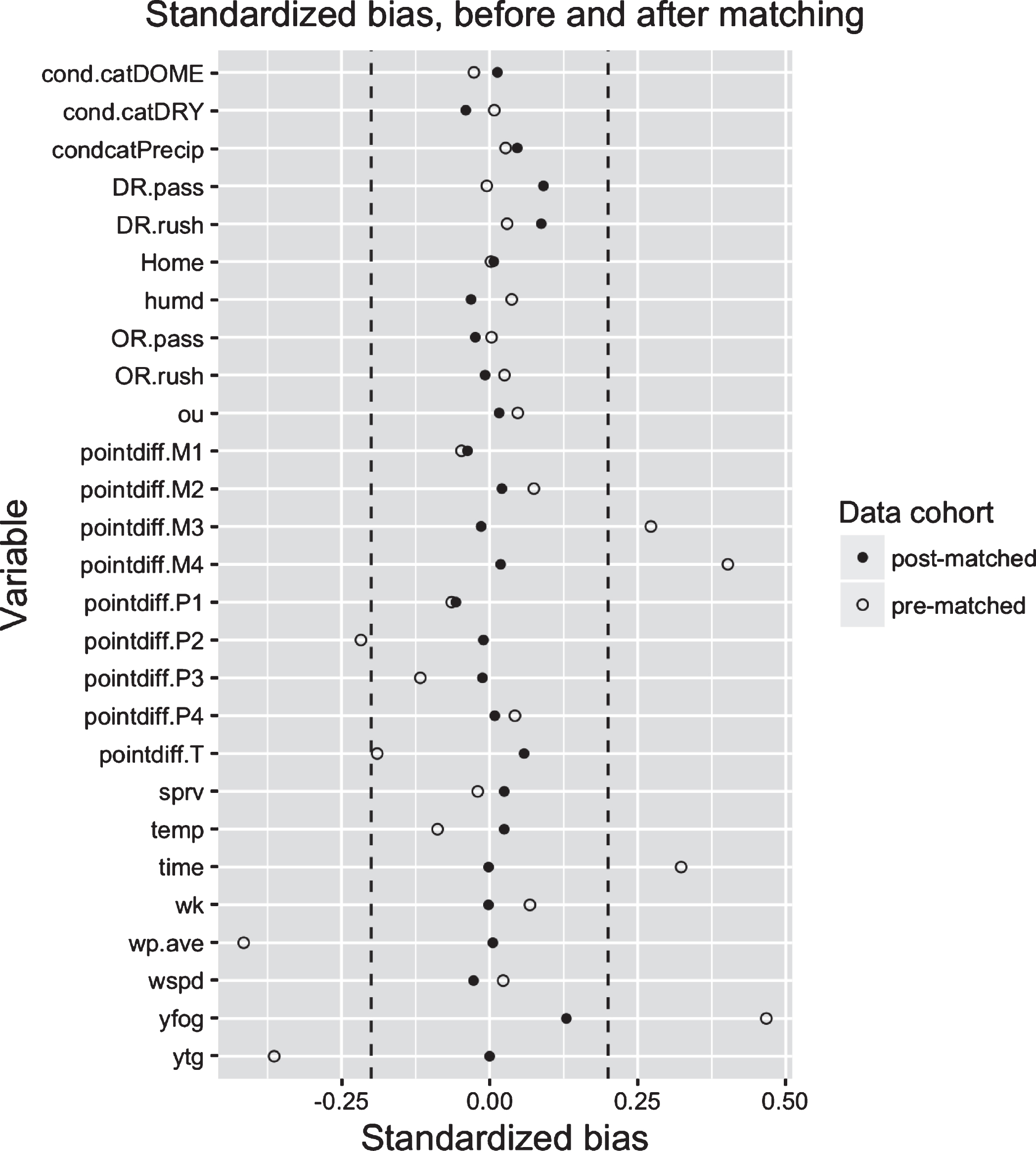
The distribution of x is considered balanced if |SBx|<0.2 (Stuart, 2010). We visualize the reduction in standardized bias after matching for the ATC using the ‘Love’ plot in Figure 4 (Ahmed et al., 2006). Prior to matching, there were seven variables outside the 0.2 threshold with respect to SBx. After matching, all variables in X fall below this threshold, suggesting our matching algorithm has effectively reduced the bias in the distributions of X.
Fig.4
‘Love’ plot of standardized bias before and after matching for the ATC. In general, the standardized bias among the matched cohort is closer to 0 than among the pre-matched cohort. For descriptions of the covariates listed, please see Table 1. Vertical dashed lines at ±0.2 are provided to reflect recommended thresholds for covariate balance.
5Results
Density curves showing Y = Δwp in each of our matched treatment and control groups are shown in Figure 5. This figure highlights several important aspects of the fourth down decision making process. First, the change in win probability for teams that did not go for it is centered at around -1%, with a relatively smaller variance. Alternatively, the curve among teams that went for it is bimodal, with positive and negative peaks reflecting successful and failed conversions, respectively. This distribution has a noticeably larger variance than the control distribution. These findings tie into the perception that coaches are risk adverse (see Section 2 in Sports), as going for it comes with greater variability in the change in win probability than not going for it.
Fig.5
Density curves for the changes in win probability on all matched fourth down plays. The average change in win probability for teams that went for it is about 1.9% higher than for teams that did not go for it (See Equation (2)). However, going for it also involves a larger variance in win probability changes, relative to not going for it.
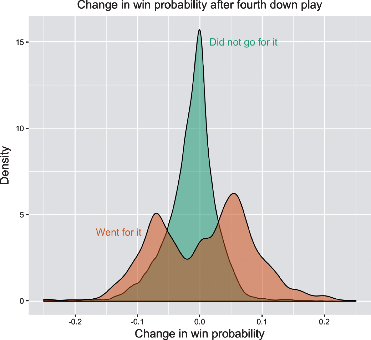
Overall, plays where teams that went for it had an average change in win probability 1.9% greater than plays where teams kicked. As judged by the Wilcoxen rank-sum test, is is unlikely that these two distributions are equivalent (p - value < .0001), signaling, across all matched plays, an added benefit to going for it on fourth down. This is unsurprising given previous findings of Romer (2006) and Burke and Quealy (2013), but reassuring given that our approach helps to correct for the multitude of differences between teams that went for it and those that did not.
Given non-normality in the distributions of changes in win probability, we use the bootstrap to estimate the distribution of each team’s TTCf. First, for each f, we identify all plays where Wi = 0, as well as the corresponding matches for those plays. We next bootstrapped 10,000 random samples of pairs with replacement, using a sample size equal to the number of matched controls for each team. The differences in Y between pairs were then summed for each f for each bootstrap sample. These aggregated changes represent estimated increases or decreases in the number of wins added between the 2004 and 2016 seasons, had f actually gone for it, instead of kicking, based on the 4th Down Bot’s recommendation.6
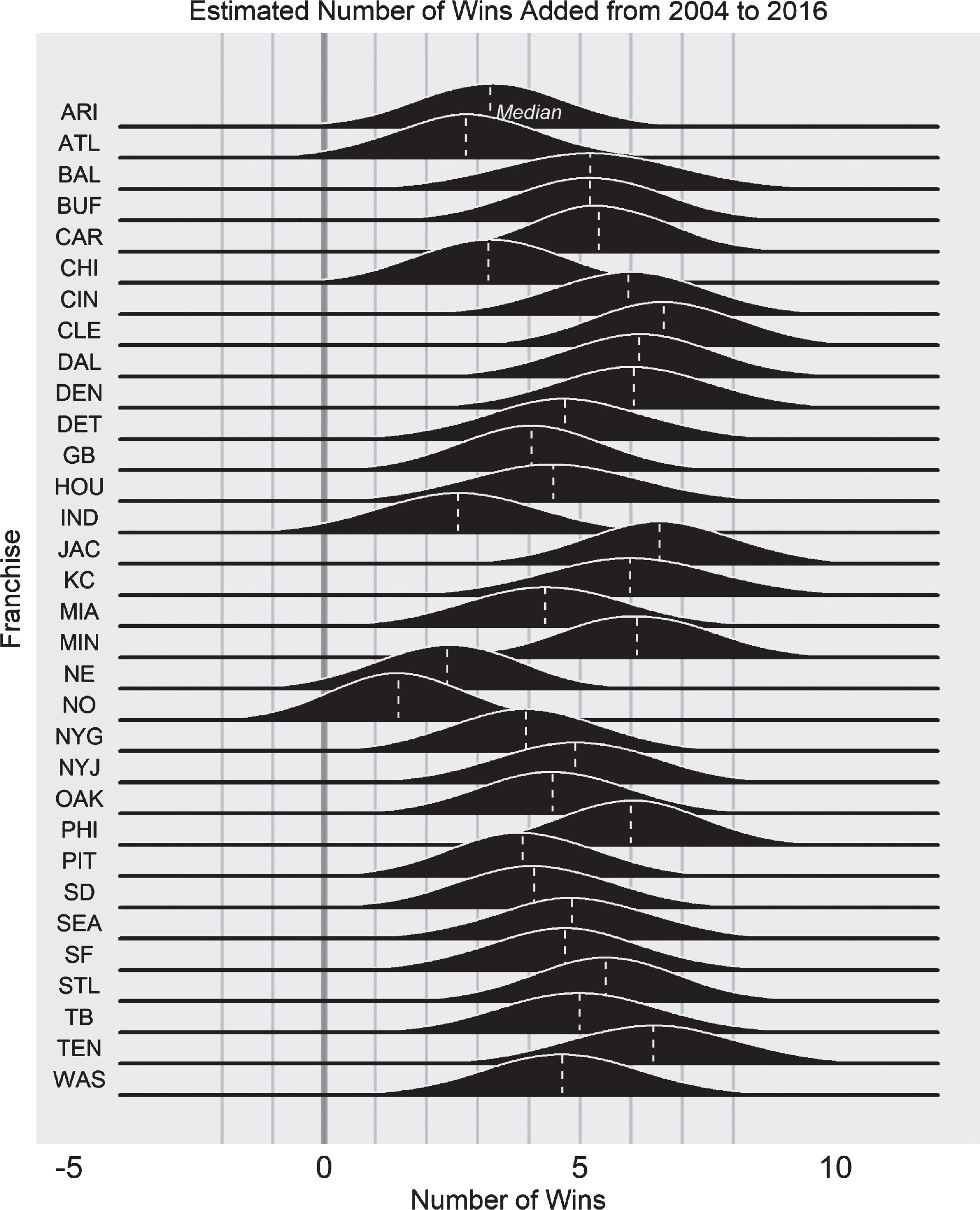
Figure 6 shows the distributions of TTCf for all f using overlaid density curves. Due to chance, we would expect about one or two teams to boast significantly positive results when using 32 comparisons at the 5% level. However, for 29 of the 32 teams, density curves in Figure 6 show a negligible overlap with 0, indicating that these franchises would have most likely added wins over the last 13 years by always going for it on fourth down in the 4th Down Bot recommended range. The mean number of wins added is roughly 4.7 wins, with a low of 1.5 wins for New Orleans and a high of 6.7 wins for Cleveland. New England, Indianapolis, and New Orleans are the only three franchises, where, among the bootstrap distributions of TTCf, it is feasible that the more aggressive strategy would not have yielded an increased win total. Anecdotally, this matches the perception that these franchises make better decisions on fourth downs (Schatz, 2015).
Fig.6
Bootstrapped results for the estimated number of wins added per team (TTCf) from 2004 to 2016, were each team to have adopted an aggressive fourth down strategy.
Results for each wp model are visualized separately in Figure 9 in the Appendix. The center for the random forest win probability model is approximately 3.6 additional wins, and the center for the generalized additive model of win probability model is approximately 5.9 additional wins. Although the magnitude of wins added differs to a certain extent, we see similarity in the team ranks based on the number of wins added under each individual win probability model.
6Discussion
In this study, we utilized methods from the Rubin Causal Method and data from 13 National Football League seasons to assess the claim that teams are too conservative in attempting fourth downs. Through the construction of a propensity score model, nearest-neighbor matching, and replications of the win probability models constructed by Lock and Nettleton (2014) and Horowitz (2016), we find that the majority of teams in the NFL would have improved their record by attempting more fourth downs, averaging a roughly 4.7 win increase over the last 13 seasons. These results broaden the scope of the fourth down analysis conducted by Romer (2006), although our final estimate of the benefit to going for it is quite similar.
In one respect, it is possible that we may be underestimating the impact of a proper fourth down strategy. The recommendations of the two-dimensional 4th Down Bot in Figure 8 are somewhat naive, and do not account for time remaining and point differential. Thus, the Bot’s model alone is likely imperfect for each NFL decision, and identifying the best decision based on variables besides yards to go and field position would likely increase the benefit of aggressive fourth down behavior.
Alternatively, by using change in win probability as our outcome, it is possible that we overestimated the number of wins that teams could have gained. For instance, going for it early in one game may result in the lack of a necessity to go for it later in that same game (if that team converted, perhaps it would not need to go for it on future fourth downs). However, in our analysis, multiple fourth down plays could be included from the same offensive unit in the same game. Altogether, an offensive unit in a given game appeared as a control an average of 1.16 times.7 Therefore, we do not expect that this summation of win probability changes within a game had a drastic impact on our final TTCf estimates.
We gave further consideration to franchise-level differences in the number of wins added. As an example, there is no obvious link between the estimated number of wins added and the rate of times that teams went for it in the 4th Down Bot ‘go for it’ range (correlation coefficient -0.11, p - value = 0.30). However, there was strong evidence of a link between wins added and the strength of a franchise, defined as each team’s winning percentage over the last 13 seasons (correlation coefficient -0.46, p - value = 0.01). Of course, teams with a higher winning percentage tend to also have larger within-game win probabilities, and thus have less of an absolute win percentage to add.
We considered if results varied based on certain types of 4th down attempts. In terms of yards to go for a first down, the greatest missed benefit came on 4th and 2 plays. On average, going for it on 4th-and-2 would have yielded an average increase in win probability of 0.7%. We also found that for 4th-and-long scenarios (yards to go greater than 4), the average change in win probability would have been 0.08% lower for teams that went for it. In terms of field position, the greatest opportunities were lost on plays closer to the offensive team’s own goal line. Within 60 yards of a team’s own end zone (which, roughly, corresponds to being out of field goal range), the missed chance to go for it corresponded with a 0.5% increase in average win probability than the actual observed kick. Alternatively, beyond that cutoff, a missed chance to go for it yielded, on average, a 0.3% decrease in average win probability. Although this highlights the areas where teams have had perhaps the most to gain by going for it on 4th down, providing a more specific strategy is beyond the scope of this paper and could require slightly different methodology.
Next, we assessed the assertion that coaches’ ability to make unbiased decisions was impaired by loss-aversion, described in Section 2 in Sports. We looked at the average change in win probability in the matched cohort based on whether or not an offensive team was winning, trailing or tied. We saw no significant difference between the score categories, implying that, at some level, the benefit to adapting an aggressive fourth down strategy holds no matter the game’s score.
As referenced in Section 3.1, any fourth down play with a penalty was dropped, a necessary step in data cleaning. For example, if a team threw a pass on fourth down and drew an interference penalty that resulted in a first down, that would be a positive and notable increase in the offensive team’s wp. Our intuition is that, on average, these positive changes would be nullified by penalties against the offense that would lead to a change in possession or push it outside of the range to attempt a fourth down.
One note that also deserves mention is that the 4th-down bot recommendation (to go for it or not, a decision based on expected points) and our outcomes (change in wp) are calculated using different statistical frameworks. As a result, we are not worried that our finding that teams should have gone for it was, by nature, the result of us using the ‘go for it’ range of plays. Another perceived limitation could be that in using the change in win probability as an outcome, we risk our estimates being unduly impacted by large jumps or drops in the final minutes of a game. However, we performed a robustness check to see if plays within the last four minutes of a game were skewing results. Stripping these plays and reviewing results, we observe nearly identical findings.
As a reminder, our results are team specific over the past 13 seasons. The estimated number of wins added reflect the number of wins that teams could have gained if it were the only team in the NFL to have followed the 4th Down Bot. If several teams were to have adopted the same strategy, the benefit for any individual team would be smaller. That said, if teams maintain their past tendencies moving forward, it is also reasonable to suggest that these findings will continue to hold.
There is some evidence that coaches can respond to academic research. In a mostly unrelated study on inefficiencies in the NFL, Kovash and Levitt (2009) identified that teams should pass more often, relative to rushing attempts. Testing the minimax theorem, the authors found that correcting this inefficiency would be worth about half a win per season. Indeed, in recent years, coaches have worked to correct this deficiency, and the 2015 season was labeled the “greatest passing season in league history" by The New York Times (Stuart, 2016).
Although our study used an outside source for a fourth down decisions (the 4th Down Bot), one benefit is that a similar methodology can be replicated with alternate strategies. This presents the possibility for future work to identify the most effective game plan. The methodology used in this paper controls for the time remaining, point differential and offensive and defensive team’s relative strengths, variables that have often been ignored, in order to produce meaningful statistical inference on fourth down attempts throughout an entire game. It is our hope that these results will help inform NFL coaches, management, and fans to the benefits of improved fourth down decision making.
AAppendix
A.1Outcome
In this section we explore the two win probability models that we used to impute our outcomes.
First, we used a near-identical random forest model to that proposed and calibrated by Lock and Nettleton (2014). Random forests (Breiman, 2001; D'ýaz-Uriarte and De Andres, 2006; Genuer et al., 2008; Liaw and Wiener, 2002; Cutler et al., 2007) grow several classification trees to learn about the relationship between predictor variables and an outcome (in our case, winning a football game). Random forests boast well-documented predictive ability, can combine unknown variable interactions in a non-linear way, assess variable importance naturally and effectively, and make minimal assumptions.
Our only deviation from Lock and Nettleton (2014) came in how we trained the model. Whereas Lock and Nettleton (2014) used a testing data set of one full year only, we randomly sampled two games from each week of each NFL season between 2004 and 2016 to be our test data (68,009 plays). All remaining plays were used for the training data (444,069 plays). Our model used all predictor variables in Table 2 and the randomForest package in R (Liaw and Wiener, 2002). As in Lock and Nettleton (2014), we used 500 regression trees, sampled two predictor variables at each split in the regression tree, and used a maximum terminal node size of 200.
Our second win probability framework stems from the ‘nflscrapR’ package in R (Horowitz, 2016), which uses a generalized additive model (GAM) to estimate the probability of the offensive team winning. GAMs can account for non-linear associations between predictors and an outcome and make fewer assumptions than ordinary least squares. We implemented a GAM using the variables in Table 2, fit via the ‘mgcv’ package in R (Wood, 2001), using a penalized likelihood approach that helps prevent overfitting. To explore the accuracy of the GAM on out-of-sample plays, we used the identical training and test data sets implemented with the random forest model described above.
Table 3
Descriptions of variables and interaction terms used in the propensity score model
| Covariate | Description | Spline knots |
| yfog | Yards from own goal | 10 |
| ytg | Yards to go for a first down | 5 |
| pointdiff | Score difference, split into nine categories (see manuscript) | NA |
| time | Elapsed time in minutes | 4 |
| condcat | Weather condition category: Precipitation, Dry, Dome | NA |
| temp | Temperature at kickoff (in degrees Fahrenheit) | 5 |
| humd | % Humidity | 5 |
| wspd | Wind speed at kickoff (in miles per hour) | 5 |
| sprv | Las Vegas Points Spread | 5 |
| ou | Las Vegas total points over-under | 5 |
| wp | pre-play win probability for the offensive team | 10 |
| Home | Factor variable for home or away | NA |
| wk | Week of the season | 4 |
| OR . pass | Offensive team’s pass offense rating from Football Outsiders | 5 |
| OR . rush | Offensive team’s rush offense rating from Football Outsiders | 5 |
| DR . pass | Defensive team’s pass defense rating from Football Outsiders | 5 |
| DR . rush | Defensive team’s rush offense rating from Football Outsiders | 5 |
| yfog * ytg | Interaction term between yards from own goal and yards to go | 10 &5 |
| yfog * time | Interaction term between yards from own goal and time remaining | 10 &4 |
| ytg * time | Interaction term between yards to go and time remaining | 5 &4 |
| time * pointdiff | Interaction term between time remaining and point differential | 4 &NA |
| yfog * time | Interaction term between yards to go and time remaining | 10 &4 |
We next assess the accuracy of both the random forest and GAM win probability models using the test data. For each model, predictions are grouped into 20 equal-sized bins, where each bin contains similar predictions with respect to the offensive team’s win probability on each play. The average predictions within each bin are then compared to the observed win percentage in that bin. For the models to be accurate, the observed and expected rates of the offensive team winning should be roughly the same within each bin.
Figure 7 shows a scatter plot of the observed and expected win rates within each bin for each model. Although there exist small fluctuations above and below the line where the true win rate equals the predicted win rate, there are no obvious systematic patterns that would signal a flaw in either model.
Fig.7
Scatter plot showing the accuracy of two win probability models, ‘Lock’ and ‘nflscrapR’, obtained from Lock and Nettleton (2014) and Horowitz (2016), respectively. Each dot compares the observed (using each model’s predictions) and expected (using game outcomes) win rate within 20 equal-sized bins. There are no noticeable deviations between the predicted and observed win rates for either model.
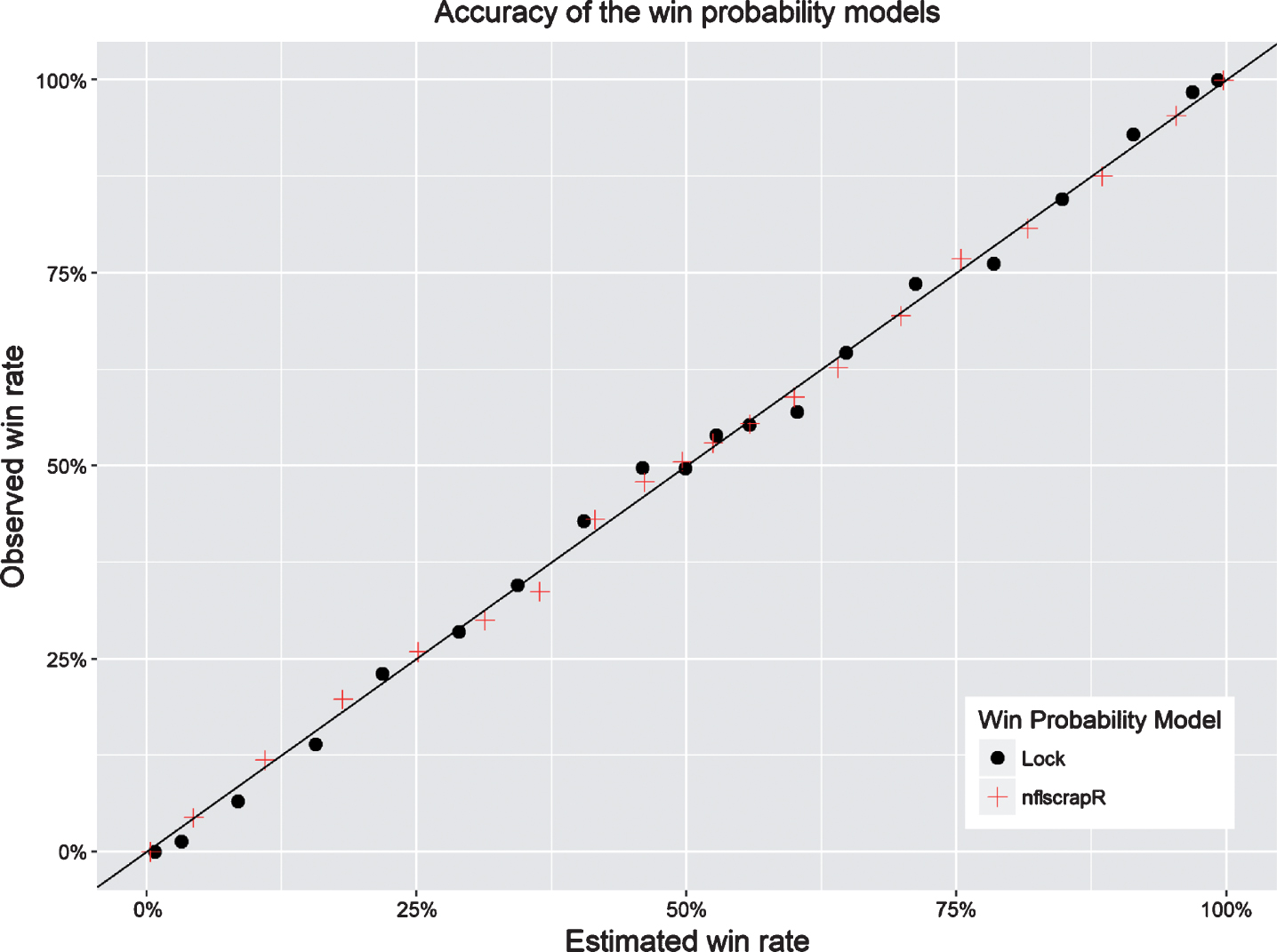
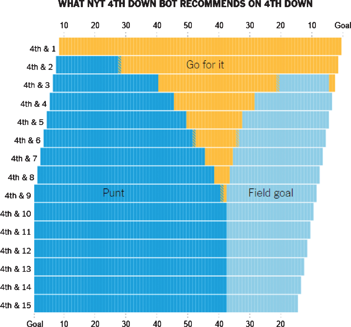
Fig.9
Bootstrapped results for the estimated number of wins added per team from 2004 to 2016. Confidence intervals are shown for each of the two win probability models, with the overall average shown in red.

References
1 | Ahmed A. , Perry G.J. , Fleg J.L. , Love T.E. , Goff D.C. , & Kitzman D.W. , (2006) , Outcomes in ambulatory chronic systolic and diastolic heart failure: A propensity score analysis, American Heart Journal, 152: , 956–966. |
2 | Breiman L. , (2001) , Random forests, Machine Learning, 45: , 5–32. |
3 | Burke B. , Carter S. , Daniel J. , Giratikanon T. , & Quealy K. , (2013) , 4th Down: When to Go for It and Why, https://www.nytimes.com/2014/09/05/upshot/4th-down-when-to-go-for-it-and-why.html?_r=0, accessed March 20, 2017. |
4 | Burke B. , & Quealy K. , (2013) , How Coaches and the NYT 4th Down Bot Compare, http://www.nytimes.com/newsgraphics/2013/11/28/fourth-downs/post.html, accessed June 21, 2017. |
5 | Carter V. , & Machol R.E. , (1978) , NoteOptimal strategies on fourth down, Management Science, 24: , 1758–1762. |
6 | Causey T. , Katz J. , & Quealy K. , (2015) , A Better 4th Down Bot: Giving Analysis Before the Play, A Better 4th DownBot: Giving Analysis Beforethe Play, accessed December 21, 2017. |
7 | Cochran W.G. , & Chambers S.P. , (1965) , The planning of observational studies of human populations, Journal of the Royal Statistical Society. Series A (General), 128: , 234–266. |
8 | Cutler D.R. , Edwards T.C. , Beard K.H. , Cutler A. , Hess K.T. , Gibson J. , & Lawler J.J. , (2007) , Random forests for classification in ecology, Ecology, 88: , 2783–2792. |
9 | Dehejia R.H. , & Wahba S. , (1999) , Causal effects in nonexperimental studies: Reevaluating the evaluation of training programs, Journal of the American statistical Association, 94: , 1053–1062. |
10 | Díaz-Uriarte R. , & De Andres S.A. , (2006) , Gene selection and classification of microarray data using random forest, BMC Bioinformatics, 7: , 3. |
11 | Garber G. , (2002) , Fourth-down analysis met with skepticism, http://static.espn.go.com/nfl/columns/garber_greg/.html, accessed March 21, 2017. |
12 | Genuer R. , Poggi J.-M. , & Tuleau C. , (2008) , Random Forests: Some methodological insights, arXiv preprint arXiv:0811.3619. |
13 | Horowitz M. , (2016) , Win Probabiity and Expected Point Functions for PBP, https://github.com/maksimhorowitz/nflscrapR/blob/master/R/ExpectedPointAndWinProbability.R, accessed June 21, 2017. |
14 | Imbens G.W. , & Rubin D.B. , (2015) , Causal Inference for Statistics, Social, and Biomedical Sciences: An Introduction, New York, NY, USA: Cambridge University Press. |
15 | Kovash K. , & Levitt S.D. , (2009) , Professionals do not play minimax: Evidence from major League Baseball and the National Football League, Tech Rep, National Bureau of Economic Research, (2009) . |
16 | Lewis M. , (2006) , If only I had the nerve, http://www.espn.com/espnmag/story?id=, accessed December 20, 2017. |
17 | Liaw A. , & Wiener M. , (2002) , Classification and regression by randomForest, R News, 2: , 18–22. |
18 | Lock D. , & Nettleton D. , (2014) , Using random forests to estimate win probability before each play of an NFL game, Journal of Quantitative Analysis in Sports, 10: , 197–205. |
19 | Lopez M.J. , & Gutman R. , (2017) , Estimation of causal effects with multiple treatments: A review and new ideas, arXiv preprint arXiv:1701.05132. |
20 | Massey C. , & Thaler R.H. , (2013) , The loser’s curse: Decision making and market efficiency in the National Football League draft, Management Science, 59: , 1479–1495. |
21 | Moskowitz T. , & Wertheim L.J. , (2012) , Scorecasting: The Hidden Influences Behind How Sports Are Played and Games Are Won, New York, NY, USA: Three Rivers Press. |
22 | Owens M.F. , & Roach M. , (2017) , Decision-making on the hot seat and the short list: Evidence from college football fourth down decisions. |
23 | Romer D. , (2006) , Do firms maximize? Evidence from professional football, Journal of Political Economy, 114: , 340–365. |
24 | Rosenbaum P.R. , & Rubin D.B. , (1983) , The central role of the propensity score in observational studies for causal effects, Biometrika, 70: , 41–55. |
25 | Rubin D.B. , (1974) , Estimating causal effects of treatments in randomized and nonrandomized studies, Journal of Educational Psychology, 66: , 688. |
26 | Schatz A. , (2015) , Aggressiveness Index: 2014, http://www.footballoutsiders.com/stat-analysis//aggressiveness-index-. |
27 | Sekhon J.S. , (2008) , Multivariate and propensity score matching software with automated balance optimization: The matching package for R, Journal of Statistical Software, Forthcoming. |
28 | Stuart C. , (2016) , N.F.L. Completes Greatest Passing Season in League History, https://www.nytimes.com/2016/01/05/sports/football/nfl-completes-greatest-passing-season-in-league-history.html?_r=0, accessed December 21, 2017. |
29 | Stuart E.A. , (2010) , Matching methods for causal inference: A review and a look forward, Statistical Science: A Review Journal of the Institute of Mathematical Statistics, 25: , 1. |
30 | Tversky A. , & Kahneman D. , (1991) , Loss aversion in riskless choice: A reference-dependent model, The Quarterly Journal of Economics, 106: , 1039–1061. |
31 | Urschel J.D. , & Zhuang J. , (2011) , Are NFL coaches risk and loss averse? Evidence from their use of kickoff strategies, Journal of Quantitative Analysis in Sports, 7: , 2011. |
32 | Wood S.N. , (2001) , mgcv: GAMs and generalized ridge regression for R, R News, 1: , 20–25. |
Notes
1 See Rosenbaum and Rubin (1983); Stuart (2010); Lopez and Gutman (2017) for more details regarding the use of matched methods with propensity scores.
2 Armchair Analysis also provides data for games between 2000 and 2003. However, data recording for those years was not as proficient, lacking consistent recordings for, among other variables, game time, temperature, humidity and wind speed.
3 For more information, see http://www.footballoutsiders.com/info/methods
4 This data can be purchased from AA for a nominal fee, at which point it is possible to replicate our work.
5 As an example, if there were two teams with e (X) =0.5, but one had a pre-snap wp = 10% and the other had a pre-snap wp = 90%, then the first observation would have a potential change in win probability that is substantially different than the second observation, which would complicate an analysis that matches on e (X) alone.
6 As we discuss in Section 6, TTCf more closely reflects the increased wins if only team f had adopted the aggressive fourth down strategy. If several teams were to have adopted the more aggressive approach, the marginal benefit for each team would be lower.
7 Our matched cohort included 7,698 controls. With 13 regular seasons of games, where each of 32 teams played 16 games apiece, there were potentially 3,328 games and 6,656 offensive units that could have appeared.


