
A metric to measure dynamic competitive balance with respect to prize concentration
Abstract
This study establishes the k index to measure the level of dynamic competitive balance (CB) in a sports league. It also introduces the concept of memory span in measuring dynamic CB. The k index reflects the contemporaneous level of dynamic CB at each season in the history of a league as equivalent to that of a league where k teams have equal chances of winning the title. All seasons of selected European and South American domestic soccer leagues, continental soccer cups, and those of the NBA were analyzed with respect to their k index.
1.Introduction
Competitive balance (CB henceforth) is a subject vastly scrutinized in the sports economics literature. The interest in CB stems from the uncertainty of outcome hypothesis (Rottenberg, 1956). CB is a multi-dimensional continuous variable — i.e. there are levels of CB and, depending on what type of data it is based on, they may have widely different meanings. The level of CB is directly proportional to the magnitude of randomness in the performance of the teams constituting a league regardless the dimension. Owen (2014) classifies CB into two dimensions: static and dynamic, where static refers to CB metrics based on data of a single season while dynamic refers to CB metrics based on data of multiple seasons. Evans (2014) uses the terms concentration and dominance instead, where the former relates to static CB and the latter to dynamic CB. The term concentration speaks for how leveled a season was among its participants while dominance speaks for how often the same teams win the title or finish at the first n-positions across seasons. The caveat is that static CB metrics can be calculated for several seasons and put in chronological order to represent the league history. Even in this case, a sense of dynamic CB is not conveyed because static metrics are season specific while dynamic ones can be team specific. As pointed out by Buzzacchi, Szymanski, & Valletti (2003), dynamic CB metric reveals whether particular teams dominate the championship over time and that it is of interest to many sports fans.
The debate between static and dynamic CB may be defined as follows via reductio ad absurdum. Which is the least undesirable scenario: to have always a tightly disputed season with the same team being the champion for all seasons; or always a runaway winner with a new team being the champion every season? Given that the former scenario constitutes an impossible condition for a league to exist and, therefore, is the most undesirable one, it is very unlikely that the two dimensions of CB can be so independent of each other to the extent that these two extreme scenarios could ever be feasible.
With regards to dynamic CB metrics, they usually measure the turnover of teams placed at the first n-positions. When n = 1, the dynamic metric measures prize concentration (Owen, 2014). Tracking the turnover for n >1 is important, for instance, in European domestic soccer leagues as the first positions grant teams qualification for pan-European tournaments such as the Champions League — i.e. qualification is a sort of a prize per se (Manasis & Ntzoufras, 2014).
Perhaps, the most used metric for prize concentration is the Herfindahl-Hirschman Index (Herfindahl, 1950), a.k.a. HHI. The problem with the HHI for measuring dynamic CB in sports leagues — e.g. as described in Leeds & von Allmen (2016, p. 164) — is that it was originally devised to measure market share concentration among firms within a fixed pre-specified time interval — e.g. within a year, a static measure — and not to measure how this concentration evolved over time — e.g. year by year, a dynamic measure. Thus, its insertion into the CB context requires that a range of seasons be defined for it to be calculated for dynamic purposes — i.e. using data from multiple seasons. The definition of this range of seasons seems to be based on convenience — typically decadal or decennial (Humphreys, 2002) (Kringstad & Gerrard, 2007).
This study demonstrates how the choice of the range of seasons for the calculation of the HHI impacts the very matter itself or its inverse (HHI-1) are intended to measure: how many teams equally likely to win the title would be required to result in the same level of dynamic CB observed across past seasons of a league. It also puts forth a standardized manner to set the range of seasons to measure dynamic CB in the form of the k index.
First, an elaboration of the concept of memory span is presented given that its comprehension is key to the understanding of why it should be incorporated in a new dynamic CB metric. Next, the formula for the k index is introduced and a demonstration of how it compares to the HHI-1 via simulation is provided. In order to demonstrate how the idea proposed by this study plays out in the real world, the history of selected soccer leagues and that of the NBA is then analyzed from the perspective of the k index. Lastly, a sensitivity analysis is performed as to depict the impact of the memory span magnitude on the k index.
2.The concept of memory span
Measuring dynamic CB in sports leagues may be compared to measuring dynamic CB in the following scenarios of a ball drawing experiment.
Scenario1: Balls are drawn with replacement from an urn with m different ball colors. If all colors have the same probability of being drawn, an observer of this experiment would be able to estimate dynamic CB between colors just by estimating m after several trials of this experiment. The analogy to a sports league is that each color is one of the teams truly competing for the title — i.e. not all teams playing the league — and every trial is a season.
The expectation of the number of colors observed until the tth trial in this case is:
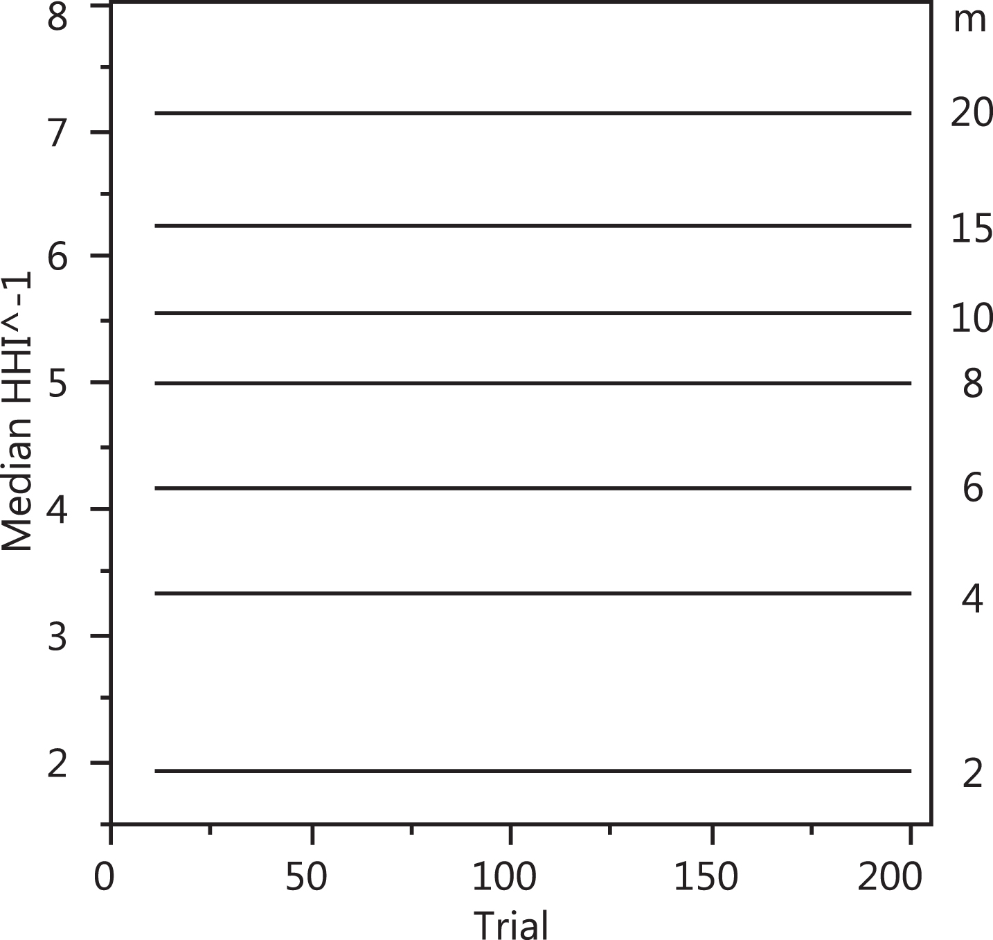
Figure 1(a) shows E (mt) as function of t for t = 10, 20, 30, 40, and 50; and for m between 1 to 20. Consider the case for t = 10 (i.e. 10 seasons) which is the range of seasons commonly associated with the HHI. The E (mt) reflects m well up to m = 3. As m increases, the bias between m and E (mt) increases, as observed in Fig. 1(b). For instance, it is observed that for m = 10, E (mt) is approximately 6.5 for t = 10, a bias of 35. For t = 50, biases are below 10 up to m = 20.
Fig.1
(a) Expectation of m at trial t vs. m; (b) Bias [m - E(mt)]/m; both for t = 10, 20, 30, 40, and 50.
![(a) Expectation of m at trial t vs. m; (b) Bias [m - E(mt)]/m; both for t = 10, 20, 30, 40, and 50.](https://content.iospress.com:443/media/jsa/2019/5-3/jsa-5-3-jsa180323/jsa-5-jsa180323-g001.jpg)
Thus, the observer of the experiment under Scenario 1 would considerably underestimate m unless the estimation of m is made at a trial t much larger than m – e.g. for t = 2m, the underestimation is approximately 13%. Hence, while trials are performed, the greater the observed number of different colors being drawn from the urn, the proportionally longer the observer needs to wait to estimate m for a given bias — i.e. the observer’s memory span needs to be proportional to the observed number of colors. This insight is also applicable to the HHI as follows.
Eq (1) shows the HHI formula to be applied for the ball experiment outcomes in analogy to a sports league:
(1)
• HHIt,n is the HHI from trial t – n + 1 to trial t
• n is the number of trials (i.e. interval) considered (i.e. the memory span)
• Ct,n is the set of the colors i = 1, 2, …, m that were drawn from trial t – n + 1 to trial t
• Wij equals 0 if the ith color belonging to Ct,n was not drawn at trial j, or 1 if it did
The inverse of the HHI (i.e. HHI-1) should then represent the number of colors (teams) that are present in the urn (competed for the title), from trial (t – n + 1) to t, and with equal probability of being drawn (of winning).
Leveraging from Hill (1973), consider that pi is the proportion of times the ith color was drawn from trial (t – n + 1) to t for i = 1, 2, …, m. Thus:
And the inverse of this (weighted) average proportion of a color being drawn is the equivalent number of different colors in the urn with equal probability of being drawn, an estimate of m.
By “equal probability” it is not meant that the index can only be applied to ludic situations like this urn example. Instead, “equal probability” is used to be in accordance with the fact that it is an inverse of an average.
The urn examples here do not use unequal probabilities of colors being drawn just because that would add unnecessary complexity to the understanding of the memory span.
Thus, for a given number of trials n, observing (a) three colors with proportions 1/3, 1/3, and 1/3, or (b) four colors with proportions 0.44, 0.34, 0.11, and 0.11, or yet (c) five colors with proportions 0.52, 0.18, 0.10, 0.10, and 0.10 would imply that the level of competition among colors in (b) and (c) is “equivalent” to that in (a) because HHI-1 ∼ 3 in all three situations regardless whether colors had the same probability of being drawn — hence the word “equivalent”.
Using a decennial interval (i.e. n = 10) in eq (1), a moving HHI-1 can be calculated season by season from trial t = 10 to 200. The experiment under Scenario 1 was simulated one thousand times for an epoch of 200 trials for each of the following levels of m: 2, 4, 6, 8, 10, 15, 20. The median
Fig.2
Median HHI-1t,10 vs. trial for m = 2, 4, 6, 8, 10, 15, and 20; the levels of m depicted here were selected for their flat profile across the 200 trials when n = 10 in order to convey a neater plot; whether the profile of the median HHI-1t,n is flat or not across the 200 trials is a function of the combination of the n and m levels.
It is observed in Fig. 2 that the median
Scenario 2: It is the same as Scenario 1 except that new ball colors are inserted into and removed from the urn with unknown frequency and in a concealed manner. This is to represent that in a sports league some teams may have their heyday for a while only — i.e. “to belong to the urn and then leave it”. They may also temporarily return to the urn sometime after they leave. So, within a short period of seasons they truly compete for the title, they may or may not win, and if they never win and leave the urn, the observer cannot account for them — i.e. if a new color is inserted into the urn and is never drawn until it is removed from it, it will not be seen by the observer.
As such, the concealed insertion and removal of colors pose two new issues related to the underestimation of m at trial t. First, the idea that the estimated m faithfully represents dynamic CB falls apart. Estimating m or
For instance, the ball experiment under Scenario 2 was simulated one thousand times for an epoch of 200 trials with: m = 24 from trial 1 to 50; m = 12 from trial 51 to 100; m = 6 from trial 101 to 150; and m = 3 from trial 151 to 200. I.e. nine colors left the urn before trial 51, three colors left before trial 100, and three left before trial 150. This sequence of m values obeyed a power law to represent a winner-takes-all context. The m values were set to change at every 50 trials to emphasize the difference in HHI-1t,n values between following memory spans: 10, 25, and 50. A summary of the results is shown in Fig. 3.
Fig.3
Median HHI-1t,n vs. trial for annotated memory spans n = 10, 25, 50 trials; dashed-line represents true m vs. trial.
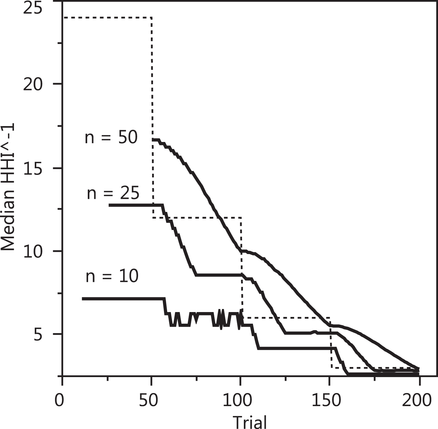
It is observed again in Fig. 3 that
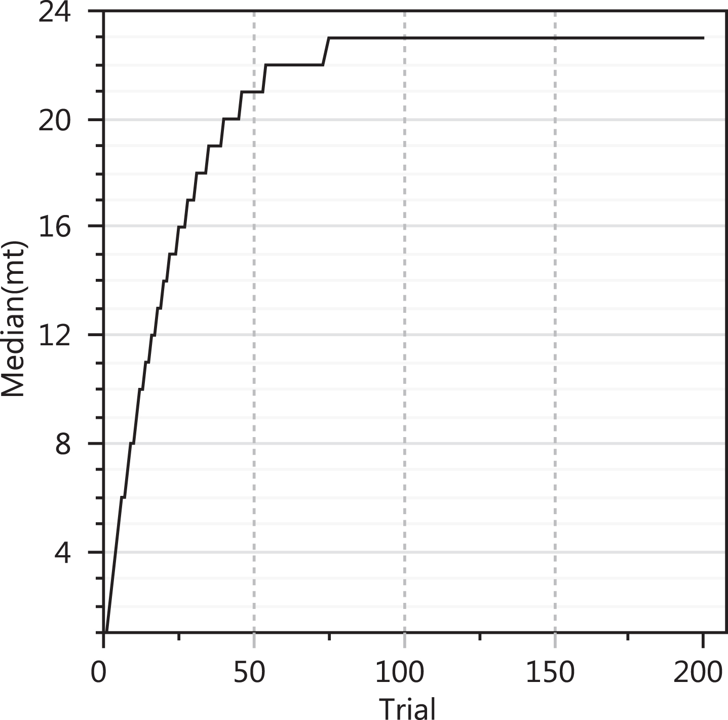
Figure 4 depicts the effect of the concealed insertion and removal of colors on the simulated results. It shows the median number of colors to be observed up to trial t (i.e. mt) vs. the number of trials. Twenty four colors had equal probability of being drawn up to t = 50 but only twenty one are observed. Two new colors are observed from t = 51 to 100. No new colors are observed from t = 101 to 200. That is, in terms of median values, one out of twenty four colors is never drawn in this simulation. More colors would be expected to be never drawn if the 50 trials interval for a change in true m was shorter.
Fig.4
Median mt vs. trials.
Therefore, the observer of the experiment can only rely on a perceived level of dynamic CB because the true one is not estimable for the reasons discussed thus far: (a) that the memory span may be either too short and largely underestimate m, or too long to be responsive to changes in true m; and (b) that the frequency and amount of new colors being inserted into and removed from the urn is unknown.
Hence, while using indices such as the HHI to measure dynamic CB, it is necessary to understand that they are about perceived dynamic CB and that the interpretation of their results is conditioned on how each specific index reflects dynamic CB perception.
For instance, back to Fig. 4, sixteen different colors are drawn by trial t = 25 in median terms. Thus, these sixteen colors dictate the perceived level of dynamic CB at t = 25, despite the point that there are twenty four in the urn. Hence, the fact that the median HHI-1t,n underestimates m in Fig. 3 is irrelevant perception-wise — i.e. the observer cannot perceive what is unseen. A key point, however, is to comprehend how the width of the memory span impacts the results and related interpretation. By trial t = 25, an observer with a memory span of 10 trials will perceive the dynamic CB of the experiment under Scenario 2 to be equivalent to one with approximately seven colors in the urn – this is because the median HHI-1t = 25,n = 10 = 7.14 in Fig. 3. By the same token, an observer with a memory span of 25 trials will perceive approximately thirteen colors in the urn. A memory span of 50 trials would force the observer to withhold judgement until t = 50.
Finally, the key point this study tries to address is which memory span should be used to compute the HHI-1t,n in order to best reflect perceived dynamic CB. For instance, under Scenario 2, which perception of dynamic CB is the correct one at trial t = 25: seven or thirteen colors in the urn? Or is it better to wait until trial t = 50 to judge it? Or something else?
The proposed general answer to this question is the following. The observer should base the width of the memory span to be used at trial t on the knowledge of how many different colors have been drawn up to trial t. If all the twenty four colors are drawn by trial t = 25, the observer should consider a wider memory span than if sixteen were drawn by the same trial. If say, only three colors are drawn by trial t = 25, the memory span should be much shorter.
The idea of an adaptive league-specific memory span is then presented in the form of the k index.
As such, the fact that “balls enter and leave the urn in a concealed manner” makes even the k index likely to underestimate true dynamic CB. This is where static CB enters the picture, because it measures how tight each season was so complementing the dynamic CB. If some teams compete for the title for a while but never win it, their impact in the overall CB can be captured only by static CB — not by the dynamic one.
3.The development of the k index
The k index is based on the HHI and is defined by eq (2).
(2)
• kt is the k index at season t
• Ct is the subset of all teams that ever won the league until season t
• wij equals 0 if the ith team belonging to Ct did not win season j, or 1 if it did
• mt is the number of different teams that have won at least one title up to season t. It is the memory span at season t— e.g. for mt = 5, the span covers season t plus the last 4 seasons; from season t = 1, until any given team does not win the title more than once, the memory span mt equals t.
kt is to be interpreted as the “equivalent” number of teams that would have truly competed for the title with equal probability of winning for the perceived level of dynamic CB at season t — just as much as the inverse of the HHI represents the same. Another metric of interest is the ratio kt/mt. It reveals the percentage of historical league winners that were still active at season t — i.e. the historical winners still “in the urn” at season t.
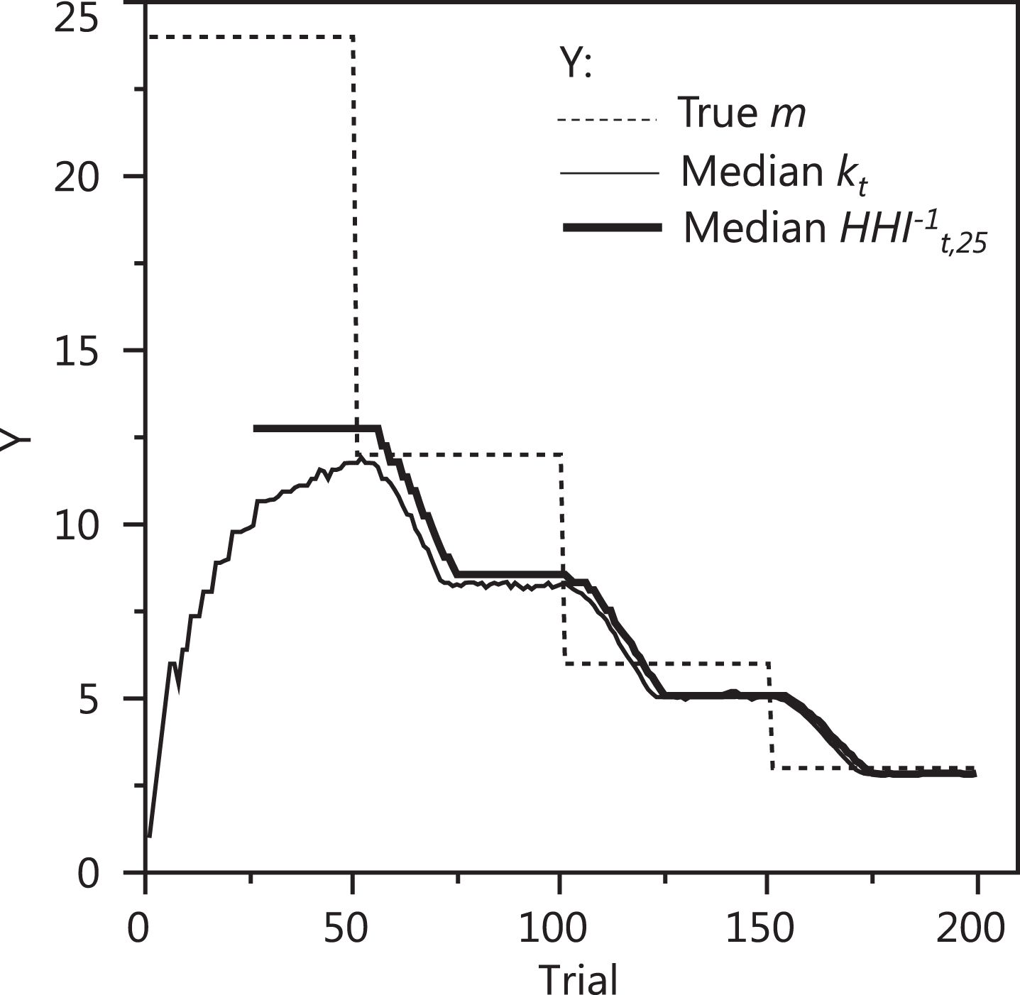
Revisiting the simulation results of the Scenario 2 of the ball experiment, Fig. 5 shows the median kt, the median HHI-1t,25 (memory span of 25 trials), and the true m across the 200 trials. It is observed that the k index is able to provide measures of dynamic CB from trial t = 1 and rises proportionally to the rate at which new colors are drawn (Fig. 4) to hit its peak around trial t = 50 where median k = 11.76 precisely. From that point on, the kt and HHI-1t,25series are much alike for both operate under similar memory spans — 23 and 25, respectively.
Fig.5
True m (dashed), median kt (thin solid), and median HHI-1t,25 (thick solid) vs. trial from the simulation results of Scenario 2.
4.Analysis of selected Leagues
Next, some selected soccer leagues were scrutinized with reference to their kt and kt/mt ratio throughout their history. For the sake of simplicity, the seasons were referred to by the year they ended — e.g. the 2015-16 season was referred to as the 2016 season. Seasons prior to and immediately after war hiatuses were treated as consecutive. This procedure was also applied when a season’s title was not awarded for any other reason other than war.
The values of kt, mt and kt/mt for all leagues within the 1998-2017 period are tabulated in the Appendix for illustrative purposes.
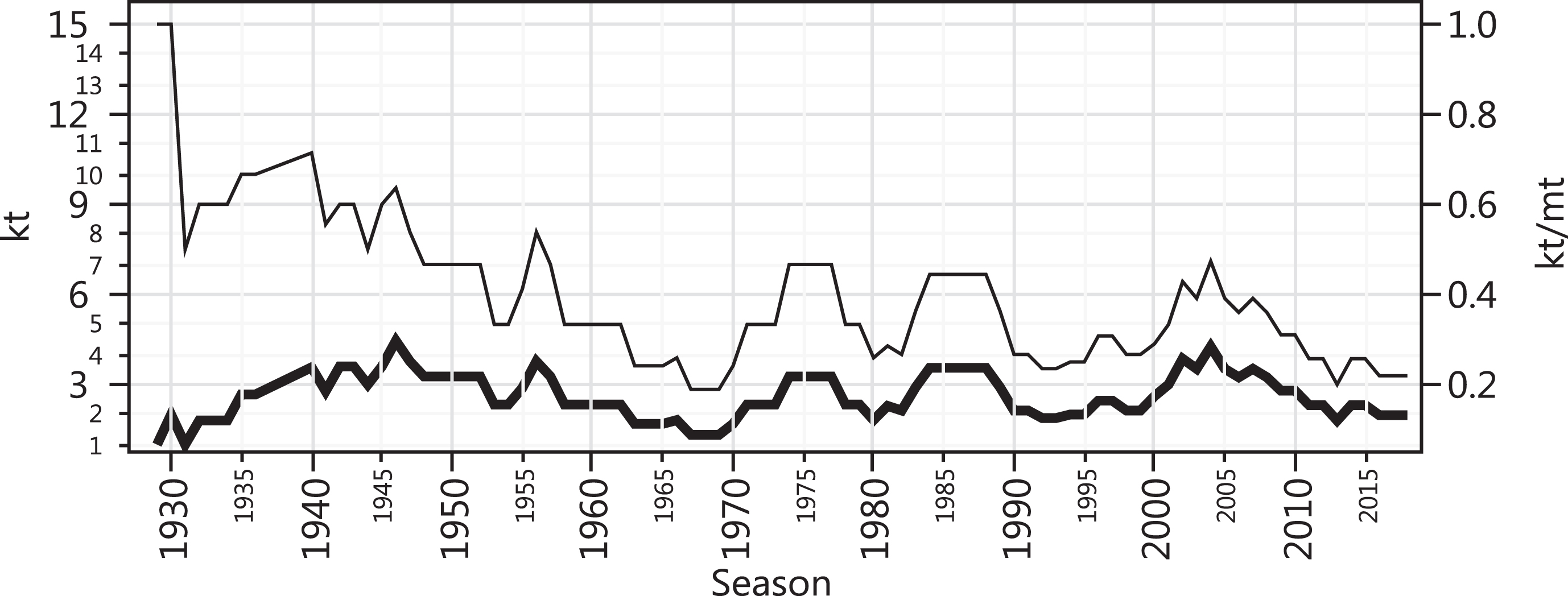
4.1The k index in Spain
The period 1929-2018 (87 seasons) is shown in Fig. 6. In 1946, the k index had reached its all-time high at 4.5 when Sevilla pulled off the title for the first time to be the 7th team to ever win it. Growth of the index past the 50’s was prevented by the build-up of the Real Madrid hegemony. They won 18 out of the 24 seasons between 1954 and 1980. This drove the index downwards to 1.8 in 1980, the lowest level in recent times. The index would still hit 4.3 in 2004 mainly due to titles won by Deportivo La Coruña in 2000 and by Valencia in 2004 & 2002. With the prominence of Barcelona between 2005 and 2018, they won 9 out of the 14 seasons, the k index dropped once again and in 2018 it was at 2.0 while 22.2% of its winners were still active — i.e. k86/m86 = 0.222 for t = 86, the 86th season of this league.
Fig.6
kt (thick) and kt/mt (thin) for the Spanish league vs. season.
4.2The k index in Italy
The period 1898–2018 (114 seasons) is shown in Fig. 7. Two titles for the 1922 season were awarded in Italy. The one for Novese was placed first and the one for Pro Vercelli second to reflect their occurrence in time.
Fig.7
kt (thick) and kt/mt (thin) for the Italian league vs. season.
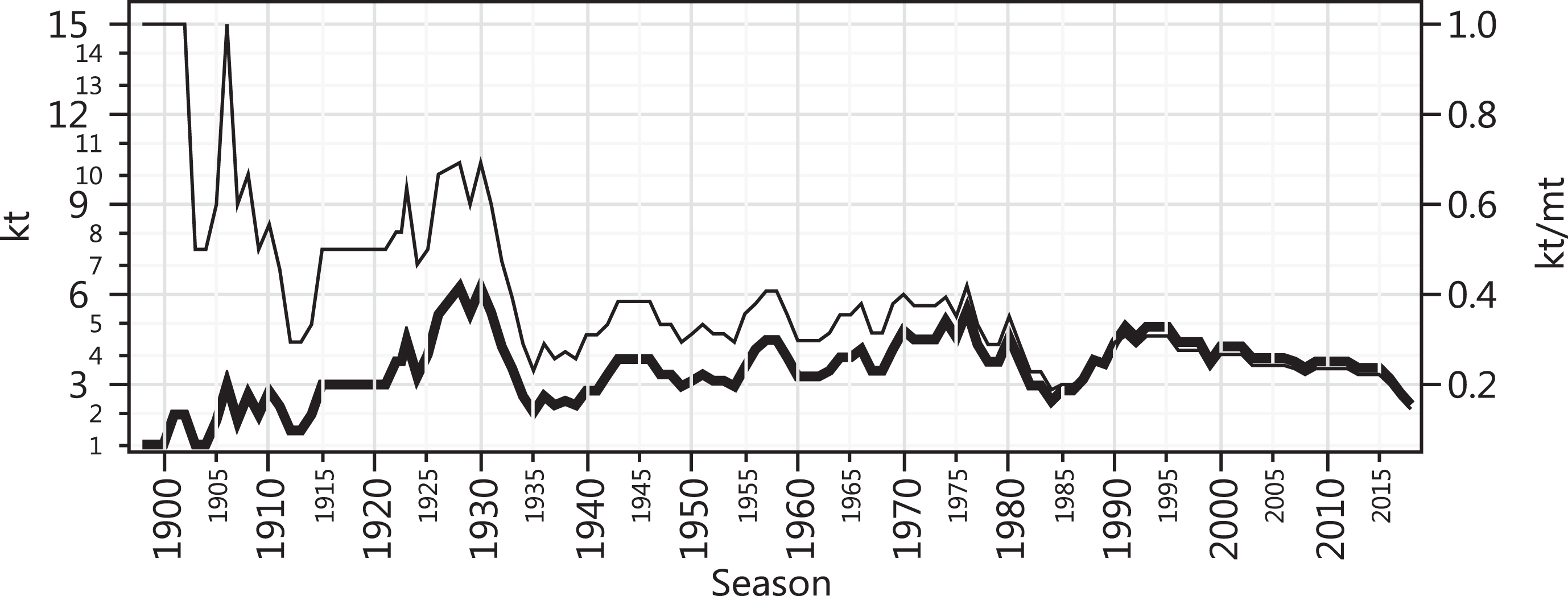
In 1929 and 1931, the k index achieved its all-time high at 5.4 with the title by Bologna and Juventus, respectively. A more recent k index high (4.9) occurred in 1991 when Sampdoria won their first Scudetto. Since then there has been a general decline and in 2018 the k index hit 2.3, its lowest level in recent times.
If it was not for the five consecutive titles by Internazionale between 2006 and 2010, much favored by the match fixing scandal which resulted in punishment to Juventus and Milan, the index could likely be even lower in 2018. Only 14.5% of the league winners were still active in 2018.
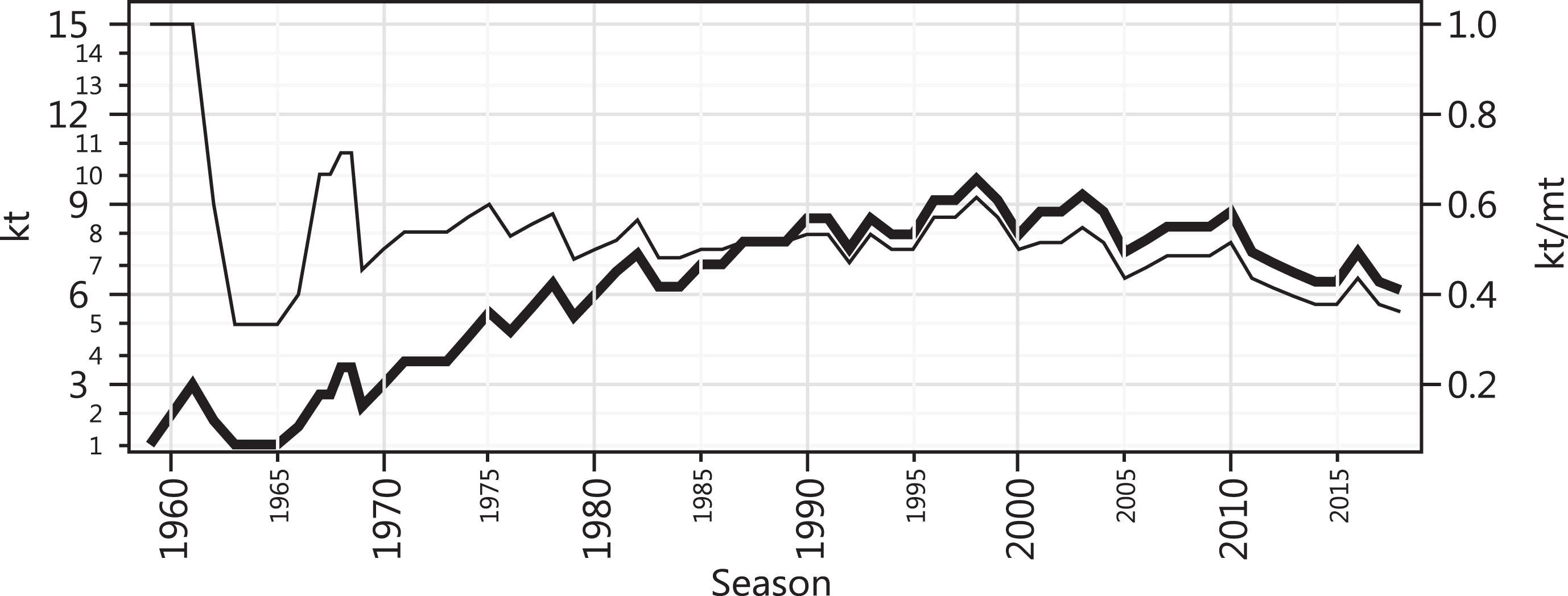
4.3The k index in England
The period 1890–2018 (119 seasons) is shown in Fig. 8. In 1962, the index reached its all-time high at 9.5 when Ipswich Town nailed their first title, the 20th team to ever win the league. This relatively high level of dynamic CB persisted until 1975 when Derby County won their second title and the k index was at 9.3.
Fig.8
kt (thick) and kt/mt (thin) for the English league vs. season.
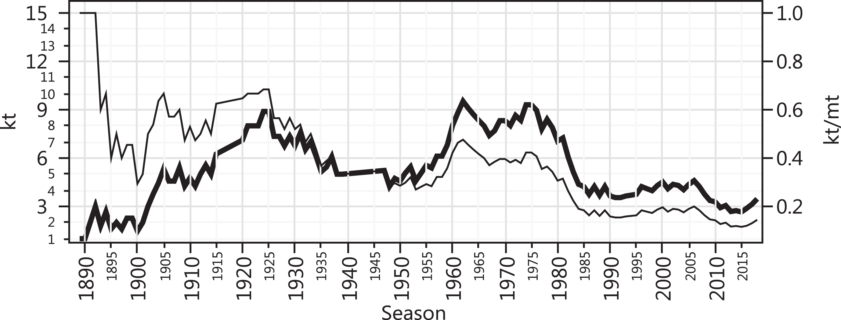
Since 1976, Liverpool and Manchester United won 10 and 13 titles respectively, out of the 43 seasons that elapsed. This was the major contributor for the index to plummet to 2.7 by 2013, its lowest level in recent times, exactly when Manchester United won their 13th title since 1976. As of 2018, the index was at 3.5. In 1992, the last year before the advent of the Premier League, the index was at 3.6. The median level of the k index during the 26 seasons under the Premier League mode thus far is at 3.75, just a little over the level in 1992. Only 14.5% of the league winners were still active in 2018.
4.4The k index in Germany
The period 1903–2018 (106 seasons) is shown in Fig. 9. The index reached its all-time high at 15.1 — remarkable for an European league — in 1971 when 28 teams had already won the title at least once in the last 59 seasons. Having a k index close to the number of participants in the league — in 1967, 18 teams played in the Bundesliga — seems to be a consequence of having an open league — with promotion and relegation between divisions — and with no big gap in quality between teams playing the major division and those playing the minor one — e.g. 1. FC Nuremberg captured the 1968 title and were relegated in 1969.
Fig.9
kt (thick) and kt/mt (thin) for the German league vs. season.
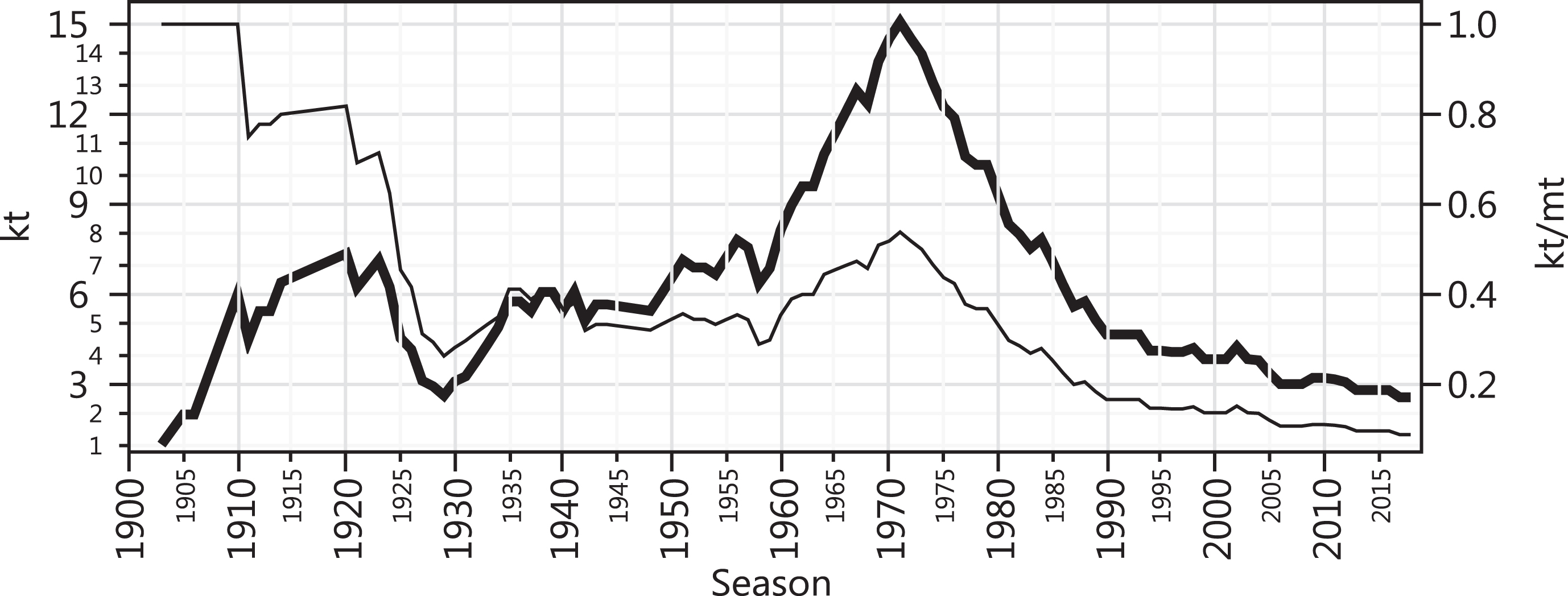
Furthermore, 53.8% of the league winners were active by 1971, the 59th season of the league. At this same point in terms of number of seasons, the Italian, the English, and the Spanish leagues had 29.7%, 32.2%, and 26.7% of active league winners, respectively.
This high level of dynamic CB was gradually reversed since then. Bayern Munich won 26 titles out of the 47 seasons between 1972 and 2018 when the k index was at 2.6, the lowest in recent times, with a mere 8.9% of league winners still active.
4.5The k index in Brazil
The period 1959–2018 (62 seasons) is shown in Fig. 10. The analysis considers results from the Taça Brasil, the Torneio Roberto Gomes Pedrosa, and the current Brasileirão to reflect CBF (Brazilian Football Confederation) records. The years of 1967 and 1968 had each two seasons in them. For these years, the winners of the Taça Brasil were placed first in time and the ones of the Torneio Roberto Gomes Pedrosa second to reproduce their real occurrence in time.
Fig.10
kt (thick) and kt/mt (thin) for the Brazilian league vs. season.
The k index all-time high was established in 1998 at 9.8 when Corinthians won their second title in the history of the league. Until 2002, the league adopted a Knock-out system to define its first positions and had a highly variable number of participating teams per season – from 20 to 116 depending on the season. The k index in 2002 was at 8.8 and 51.5% of the league winners were active. Since 2003, the European-like Round-Robin system was adopted with a more regular number of participants – 20 teams per season since 2006. In 2018, the index was at 6.1 and 36.2% of the league winners were still active — i.e. a decline trend in dynamic CB observed since the late 90’s. Yet, the k index level of 2018 was much higher than the level of the European domestic leagues studied here. The observed decline in the k index may be attributed to the Europeanisation of the league and, if so, further decline might be observed in the future until the k index approaches the 2 to 3 range, the level observed for more mature European leagues.
4.6The k index in the Champions League
The period 1956–2018 (63 seasons) is shown in Fig. 11. The period between 1956 and 1992 refers to the European Cup’s legacy.
Fig.11
kt (thick) and kt/mt (thin) for the Champions League vs. season.
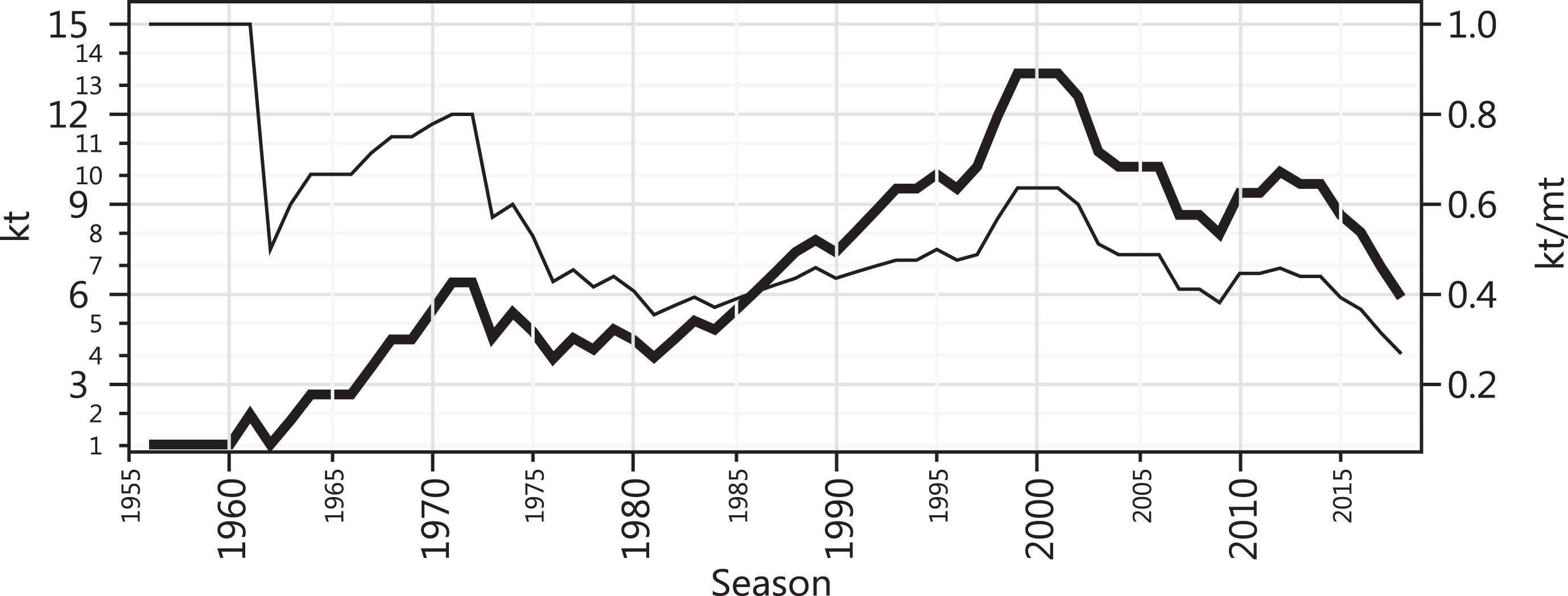
The Champions League all-time high k index (13.4) was reached in 1999 when Manchester United conquered their second title and 63.6% of the league winners were still active. Compared to the European national leagues studied here, the Champions league was no match for them in terms of dynamic CB back in the day.
The season of 1998 was the first where runners-up also qualified for the cup. The number of participating teams in the cup’s group stage inflated since then – from 16 until 1997 to 32 since 2000. As of 2018, teams placed 4th in some selected national leagues qualified directly to the group stage of the tournament. This suggests that allowing multiple teams per national association resulted in a concentration of titles among more traditional winners since 1997. Traditional European teams may not do well enough to win their national league in a given season but will hardly miss an entry to the Champions League — e.g. both Real Madrid and Barcelona can easily play the Champions League every year. This seems to have contributed to the decline in the k index since 1999. That is, relaxing the requirements for the access to the group stage seems to have resulted in a higher concentration of titles in the hands of fewer, more traditional teams — which might seem counterintuitive.
In 2018, the index was at 5.9 — i.e. suggesting a level of dynamic CB of a knock-out championship in which about 6 out of the 8 teams playing the quarterfinals have all the same chances of winning the title — and 26.8% of the league winners were still active.
4.7The k index in the Copa Libertadores
The period 1960–2017 (58 seasons) is shown in Fig. 12. The results for the 2018 season were unknown at the time of writing.
Fig.12
kt (thick) and kt/mt (thin) for the Copa Libertadores vs. season.
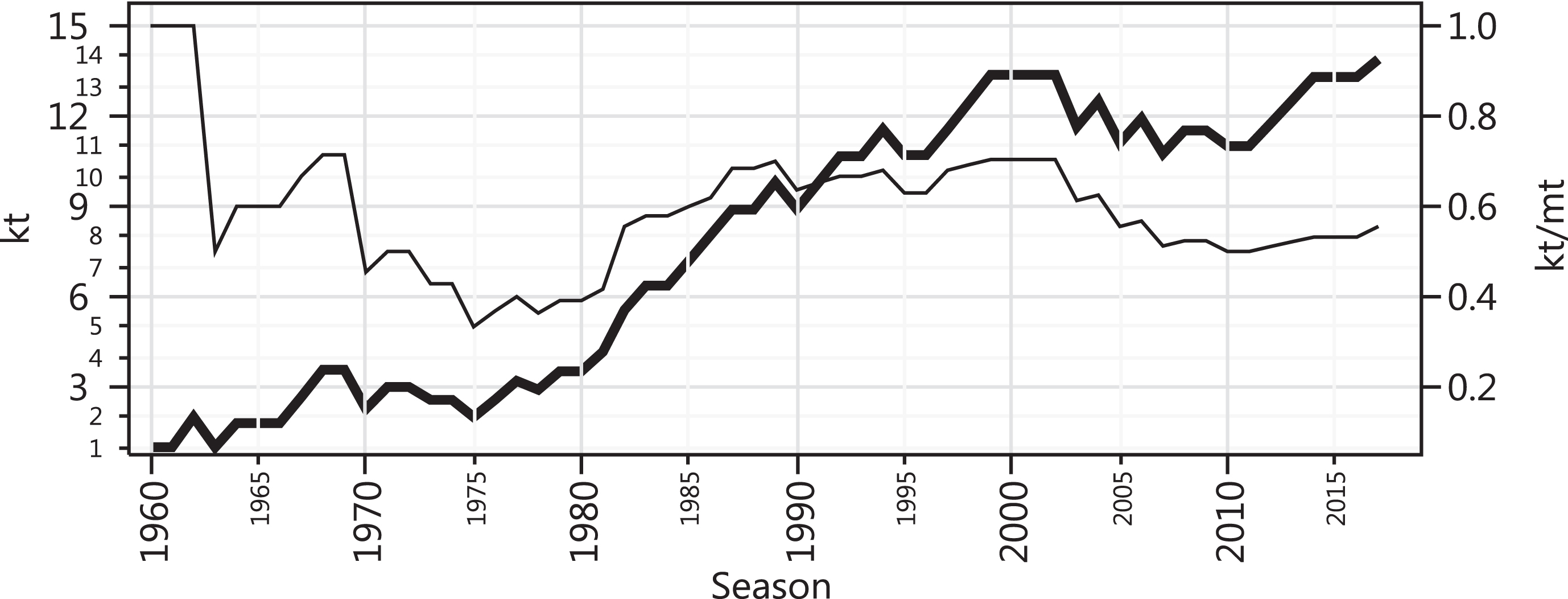
The all-time high k index (13.9) was reached as recent as in 2017 when Gremio won their third title and 55.6% of its winners were still active — about twice as high a dynamic CB as that of the Champions league in the same year. With such a high k index, the level of CB in the Copa Libertadores in 2017 was equivalent to that of a cup where about 14 teams out of the 16 that make it to the round of 16 have equal chances of winning the title.
The inflation of the number of participants also occurred in the Copa Libertadores. Up until the 1999 season, a total of 20 teams had access to the cup. Since the 2000 season, 32 teams play the group stage, excluding the 2004 season that had 36 teams. Unlike the case of the Champions League, the inflation of the number of participants has not caused the k index to undergo a clear decline thus far. Arguably, it may have ceased the growth trend in the k index since the late 70’s.
Perhaps, a continental cup with elevated levels of dynamic CB needs to be fed with teams coming from more equally balanced national leagues, like the Brazilian one.
4.8The k index in the NBA
Here the analysis of a basketball league is presented as to illustrate the application of the k index to another type of sports league, a closed one. The period 1947-2018 (72 seasons) is shown in Fig. 13. The 1947, 1948, and 1949 seasons refer to those of BBA (pre-NBA time).
Fig.13
kt (thick) and kt/mt (thin) for the NBA vs. season.
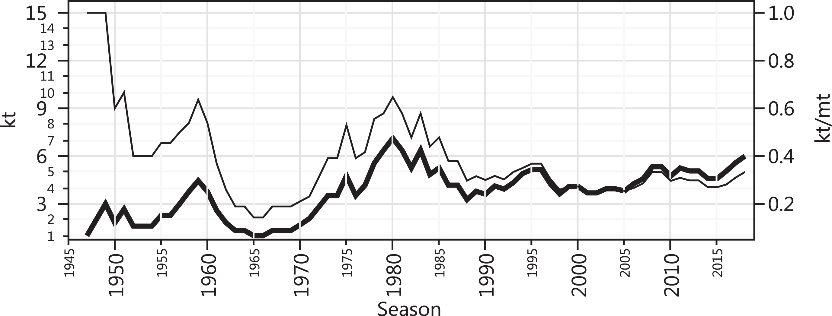
The 70’s seem to have been a decade of mounting dynamic CB in the NBA. The early hegemony of the Boston Celtics drove the k index to the value of 1 by 1966. In 1980, the index reached its all-time high at 7.1. Between 1981 and 1988, the Los Angeles Lakers (4 times) and the Boston Celtics (3 times) won together 7 titles out of the 8 seasons, and the index in 1988 sunk again down to 3.3. Since then, no sustained up or downward trend has been observed.
The k index hit the value of 6.0 in 2018, a level not observed since the early 80’s, while 33.3% of the NBA winners were still active. This means that the level of CB in 2018 was equivalent to that of a league where 6 teams out of the 8 teams participating in both East and West conference semifinals have the same chances of winning the title.
4.9Summary of the studied leagues
Figure 14 shows the k index (kt) vs. the percentage of league winners still active (kt/mt) in 2018 for all the leagues studied here; the Copa Libertadores values refer to 2017. The higher the kt /mt ratio, the lower the proportion of “dead” historical winners in a league. And, obviously, the higher the kt, the higher the amount of dynamic CB in terms of prize concentration.
Fig.14
The k index (kt) vs. the percentage of league winners still active (kt/mt) in 2018 for all the leagues studied here.
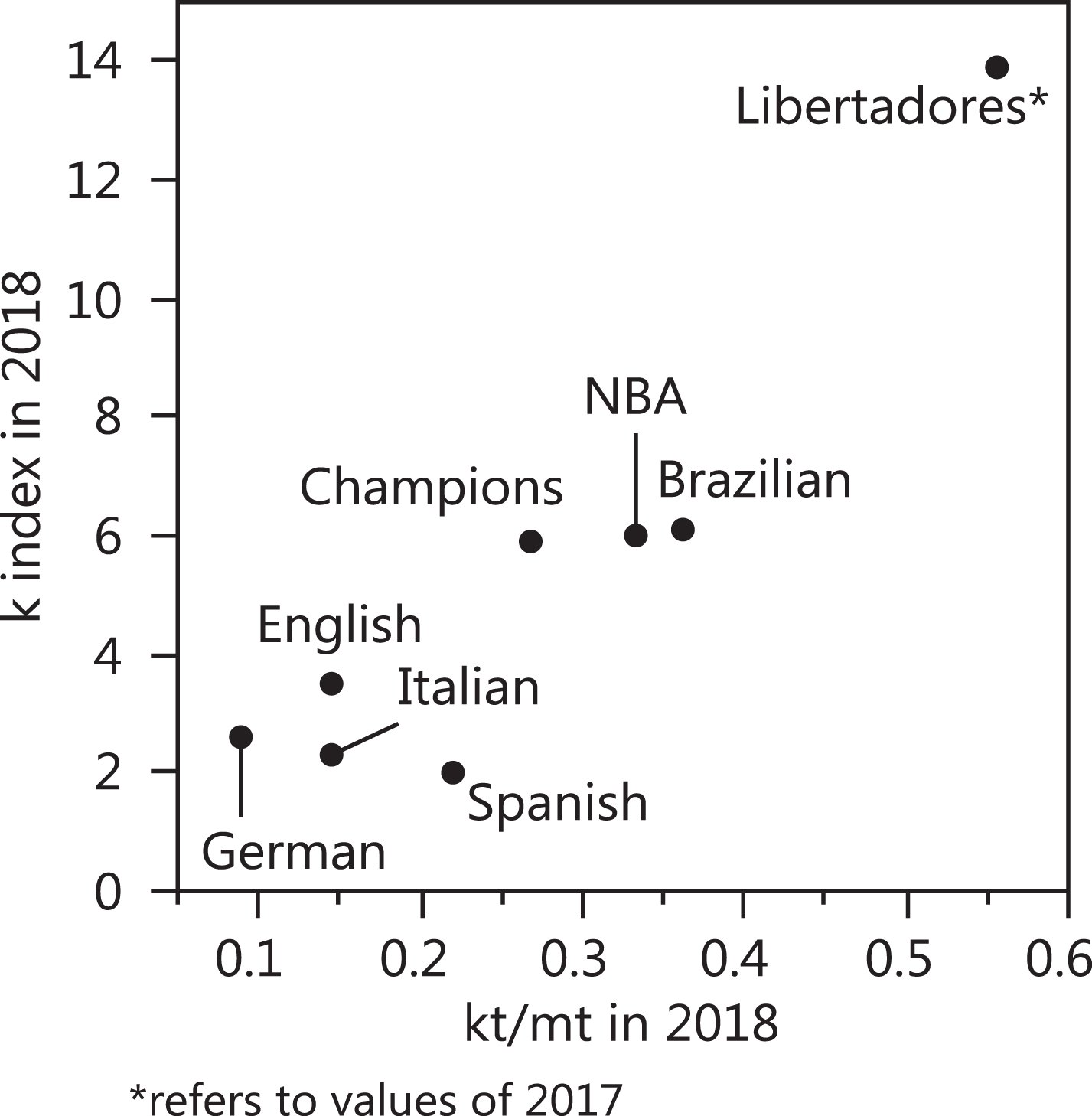
The European leagues clustered away from the other leagues for their relatively low kt and kt/mt levels. The European cluster is characterized by having a kt in the 2 to 3 range and a kt/mt in the 0.1 to 0.2 range. A second cluster contains the NBA, the Champions League, and the Brazilian league. They might form a cluster for the fact that they are not as mature as the European domestic leagues studied here — the winner-takes-all effect might be yet evolving in some of them. Lastly, the Copa Libertadores stands out as the one with highest dynamic CB and the one with a comparatively low proportion of “dead” historical winners — despite being practically as mature as the Champions League, its European counterpart.
5.k index sensitivity analysis
The memory span is the cornerstone of the k index. In eq (2), the memory span at season t (mt) is defined as the number of different teams that have won at least one title up to season t. While this definition was used for the sake of standardization, it seemed appropriate to analyze how much the k index is affected by this definition.
The plot in Fig. 15 shows the effect of varying the memory span in 2018 on the k index of this same year, with the exception of the Copa Libertadores for which the analysis refers to its k index of 2017. The memory span for each league in Fig. 15 ranges from 5 to the highest value possible — i.e. the total number of seasons of the league — in multiples of five. The “standardized by eq (2)” memory span in 2018 of each league is indicated in the caption of Fig. 15, with the exception of the Copa Libertadores for which the memory span observed in 2017 is indicated instead.
Fig.15
k index in 2018 across a range of possible mt levels by league; list of memory spans in 2018 by league as per eq 2: Spanish (9), English (24), Italian (16), German (29); Brazilian (17); Champions (22), Libertadores* (25), NBA (18).
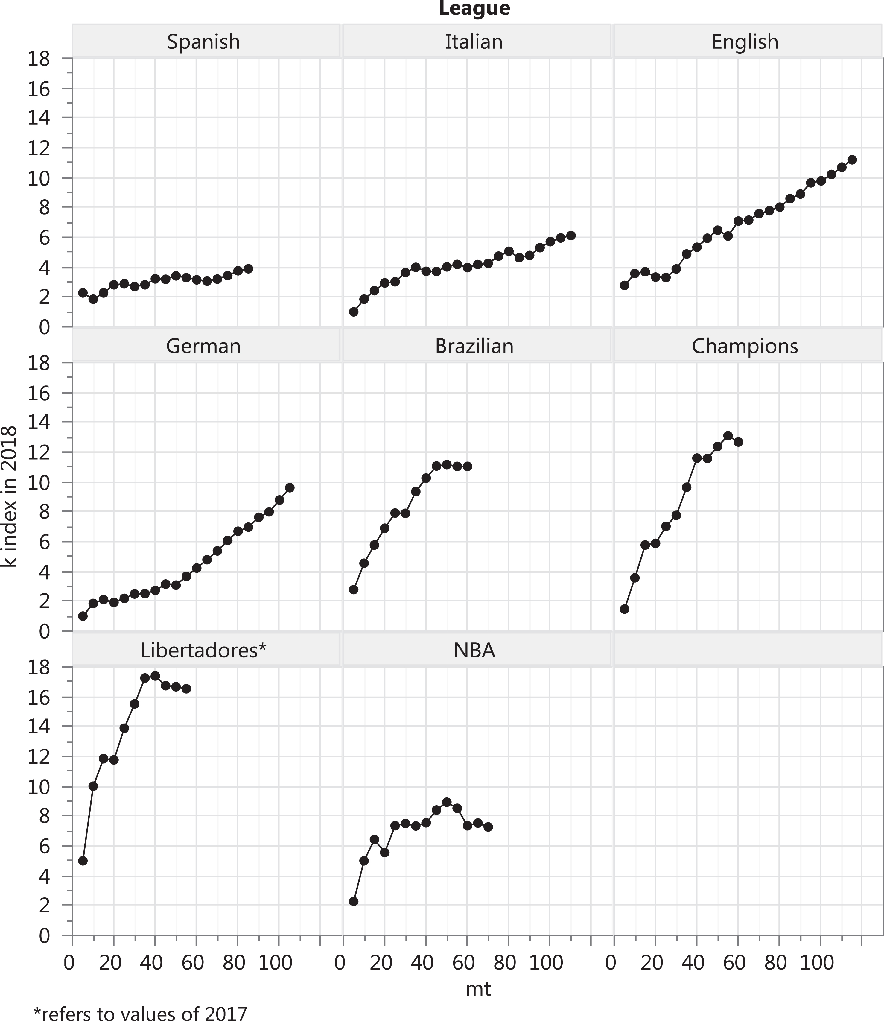
The variation of the k index as a function of the memory span in Fig. 15 shows that for mt ≤ 40 all the domestic European leagues studied here are comparatively much less affected by the variation in the memory span as their k index vs. memory span curves are much flatter. The Copa Libertadores is the most affected and the NBA’s case falls in between the extremes for mt ≤ 40. For mt >40, all curves reach a state of little or no change with the exception of the English and German leagues for which a steady curve steepness is observed.
In sum, as the “standardized by eq (2)” memory spans for all leagues studied here were well below the value of 40, it appears that the k index based on this standardized memory span – i.e. the dynamic CB in terms of prize concentration based on the standardized memory span – can be more subject to debate among observers with different memory spans in the case of the Copa Libertadores, Brazilian league, and Champions League vs. any of the European national leagues studied here, with the NBA’s case falling in-between.
6.Summary
This study demonstrated how a dynamic metric to measure dynamic competitive balance in terms of prize concentration in sports leagues was developed. The means of comparison, the k index, was defined as a modified inverse of the Herfindahl-Hirschman Index (HHI). The k index introduces the concept of a memory span to the traditional HHI. The memory span (mt) at any given season t is defined as the number of historical league winners until season t. The k index considers only the league winners and their amount of titles within the last mt – 1 seasons.
The history of selected domestic soccer leagues (Spanish, Italian, English, German, and Brazilian leagues) and of continental soccer cups (Champions League and the Copa Libertadores) were analyzed with respect to their k index. The NBA was also included in the analysis for a reference to another type of sports league.
Appendices
Appendix
Table A1
k index in the last 20 seasons per league
| Season | Spanish | English | Italian | German | Brazilian | Champions | Libertadores | NBA |
| 1998 | 2.1 | 4.0 | 4.4 | 4.2 | 9.8 | 11.9 | 12.5 | 3.6 |
| 1999 | 2.1 | 4.3 | 3.8 | 3.8 | 9.1 | 13.4 | 13.4 | 4.1 |
| 2000 | 2.6 | 4.5 | 4.3 | 3.8 | 8.0 | 13.4 | 13.4 | 4.1 |
| 2001 | 3.0 | 4.1 | 4.3 | 3.8 | 8.8 | 13.4 | 13.4 | 3.7 |
| 2002 | 3.9 | 4.4 | 4.3 | 4.3 | 8.8 | 12.6 | 13.4 | 3.7 |
| 2003 | 3.5 | 4.3 | 3.9 | 3.8 | 9.3 | 10.8 | 11.6 | 3.9 |
| 2004 | 4.3 | 4.0 | 3.9 | 3.8 | 8.8 | 10.3 | 12.5 | 3.9 |
| 2005 | 3.5 | 4.4 | 3.4 | 7.4 | 10.3 | 11.1 | 3.8 | |
| 2006 | 3.2 | 4.6 | 3.9 | 3.0 | 7.8 | 10.3 | 11.9 | 4.3 |
| 2007 | 3.5 | 4.2 | 3.8 | 3.0 | 8.3 | 8.6 | 10.8 | 4.6 |
| 2008 | 3.2 | 3.8 | 3.6 | 3.0 | 8.3 | 8.6 | 11.5 | 5.3 |
| 2009 | 2.8 | 3.4 | 3.8 | 3.2 | 8.3 | 8.0 | 11.5 | 5.3 |
| 2010 | 2.8 | 3.3 | 3.8 | 3.2 | 8.8 | 9.4 | 11.0 | 5.3 |
| 2011 | 2.3 | 2.9 | 3.8 | 3.2 | 7.4 | 9.4 | 11.0 | 5.3 |
| 2012 | 2.3 | 3.1 | 3.8 | 3.1 | 7.0 | 10.1 | 11.8 | 5.1 |
| 2013 | 1.8 | 2.7 | 3.6 | 2.8 | 6.7 | 9.7 | 13.3 | 4.6 |
| 2014 | 2.3 | 2.7 | 3.6 | 2.8 | 6.4 | 9.7 | 13.3 | 4.6 |
| 2015 | 2.3 | 2.7 | 3.6 | 2.8 | 6.4 | 8.6 | 13.3 | 4.6 |
| 2016 | 2.0 | 2.9 | 3.2 | 2.8 | 7.4 | 8.1 | 13.3 | 5.6 |
| 2017 | 2.0 | 3.1 | 2.7 | 2.6 | 6.4 | 6.9 | 13.9 | 5.6 |
| 2018 | 2.0 | 3.5 | 2.3 | 2.6 | 6.1 | 5.9 | 6.0 |
Table A2
Memory span in the last 20 seasons per league
| Season | Spanish | English | Italian | German | Brazilian | Champions | Libertadores | NBA |
| 1998 | 8 | 23 | 16 | 28 | 16 | 21 | 18 | 14 |
| 1999 | 8 | 23 | 16 | 28 | 16 | 21 | 19 | 15 |
| 2000 | 9 | 23 | 16 | 28 | 16 | 21 | 19 | 15 |
| 2001 | 9 | 23 | 16 | 28 | 17 | 21 | 19 | 15 |
| 2002 | 9 | 23 | 16 | 28 | 17 | 21 | 19 | 15 |
| 2003 | 9 | 23 | 16 | 28 | 17 | 21 | 19 | 15 |
| 2004 | 9 | 23 | 16 | 28 | 17 | 21 | 20 | 15 |
| 2005 | 9 | 23 | 28 | 17 | 21 | 20 | 15 | |
| 2006 | 9 | 23 | 16 | 28 | 17 | 21 | 21 | 16 |
| 2007 | 9 | 23 | 16 | 28 | 17 | 21 | 21 | 16 |
| 2008 | 9 | 23 | 16 | 28 | 17 | 21 | 22 | 16 |
| 2009 | 9 | 23 | 16 | 29 | 17 | 21 | 22 | 16 |
| 2010 | 9 | 23 | 16 | 29 | 17 | 21 | 22 | 16 |
| 2011 | 9 | 23 | 16 | 29 | 17 | 21 | 22 | 17 |
| 2012 | 9 | 23 | 16 | 29 | 17 | 22 | 23 | 17 |
| 2013 | 9 | 23 | 16 | 29 | 17 | 22 | 24 | 17 |
| 2014 | 9 | 23 | 16 | 29 | 17 | 22 | 25 | 17 |
| 2015 | 9 | 23 | 16 | 29 | 17 | 22 | 25 | 17 |
| 2016 | 9 | 24 | 16 | 29 | 17 | 22 | 25 | 18 |
| 2017 | 9 | 24 | 16 | 29 | 17 | 22 | 25 | 18 |
| 2018 | 9 | 24 | 16 | 29 | 17 | 22 | 18 |
Table A3
Percentage of active league winners in the last 20 seasons per league
| Season | Spanish | English | Italian | German | Brazilian | Champions | Libertadores | NBA |
| 1998 | 0.267 | 0.173 | 0.276 | 0.151 | 0.615 | 0.568 | 0.692 | 0.259 |
| 1999 | 0.267 | 0.187 | 0.235 | 0.137 | 0.571 | 0.636 | 0.704 | 0.273 |
| 2000 | 0.290 | 0.197 | 0.267 | 0.137 | 0.500 | 0.636 | 0.704 | 0.273 |
| 2001 | 0.333 | 0.178 | 0.267 | 0.137 | 0.515 | 0.636 | 0.704 | 0.246 |
| 2002 | 0.429 | 0.190 | 0.267 | 0.152 | 0.515 | 0.600 | 0.704 | 0.246 |
| 2003 | 0.391 | 0.187 | 0.242 | 0.137 | 0.548 | 0.512 | 0.613 | 0.263 |
| 2004 | 0.474 | 0.176 | 0.242 | 0.136 | 0.515 | 0.488 | 0.625 | 0.263 |
| 2005 | 0.391 | 0.190 | 0.121 | 0.436 | 0.488 | 0.556 | 0.254 | |
| 2006 | 0.360 | 0.200 | 0.242 | 0.108 | 0.459 | 0.488 | 0.568 | 0.267 |
| 2007 | 0.391 | 0.184 | 0.235 | 0.108 | 0.486 | 0.412 | 0.512 | 0.286 |
| 2008 | 0.360 | 0.163 | 0.222 | 0.108 | 0.486 | 0.412 | 0.524 | 0.333 |
| 2009 | 0.310 | 0.146 | 0.235 | 0.111 | 0.486 | 0.382 | 0.524 | 0.333 |
| 2010 | 0.310 | 0.143 | 0.235 | 0.111 | 0.515 | 0.447 | 0.500 | 0.296 |
| 2011 | 0.257 | 0.127 | 0.235 | 0.109 | 0.436 | 0.447 | 0.500 | 0.309 |
| 2012 | 0.257 | 0.133 | 0.235 | 0.106 | 0.415 | 0.458 | 0.511 | 0.298 |
| 2013 | 0.200 | 0.117 | 0.222 | 0.097 | 0.395 | 0.440 | 0.522 | 0.270 |
| 2014 | 0.257 | 0.119 | 0.222 | 0.097 | 0.378 | 0.440 | 0.532 | 0.270 |
| 2015 | 0.257 | 0.116 | 0.222 | 0.097 | 0.378 | 0.393 | 0.532 | 0.281 |
| 2016 | 0.220 | 0.120 | 0.200 | 0.097 | 0.436 | 0.367 | 0.532 | 0.281 |
| 2017 | 0.220 | 0.130 | 0.170 | 0.089 | 0.378 | 0.314 | 0.556 | 0.310 |
| 2018 | 0.220 | 0.145 | 0.145 | 0.089 | 0.362 | 0.268 | 0.333 |
References
1 | Buzzacchi, L. , Szymanski, S. , & Valletti, T.M. (2003) , Equality of opportunity and equality of outcome: Open leagues, closed leagues and competitive balance. Journal of Industry, Competition and Trade, 3: (3), 167–186. doi: 10.1023/A:1027464421241 |
2 | Evans, R. (2014) , A review of measures of competitive balance in the 'analysis of competitive balance' literature. Birkbeck Sport Business Centre Research Paper Series, 7: (2), 1–59. |
3 | Herfindahl, O.C. (1950) , Concentration in the U.S. steel industry. Unpublished doctoral dissertation, Columbia University. |
4 | Hill, M.O. (1973) , Diversity and Evenness: A unifying notation and its Consequences. Ecology, 54: (2), 427–432. doi: 10.2307/1934352 |
5 | Humphreys, B.R. (2002) , Alternative measures of competitive balance in sports leagues. Journal of Sports Economics, 3: (2), 133–148. doi:10.1177/152700250200300203 |
6 | Kringstad, M. , & Gerrard, B. (2007) , Beyond competitive balance . In: T.Slack ,M.M.Parent , International Perspectives on the Management of Sport (pp. 149–172). Burlington, MA: Elsevier Academic Press. |
7 | Leeds, M.A. , & Allmen, P.v. (2016) , The Economics of Sports (4th ed.). New York, NY: Routledge. |
8 | Manasis, V. , & Ntzoufras, I. (2014) , Between-seasons competitive balance in European football: Review of existing and devel-opment of specially designed indices. Journal of Quantitative Analysis in Sports, 10: (2), 139–152. doi:10.1515/jqas-2013-0107 |
9 | Owen, P.D. (2014) , Measurement of competitive balance and uncertainty of outcome. In GoddardJ. & SloaneP. , Handbook on the Economics of Professional Football (pp. 41–59) Chel-tenham:Edward Elgar. |
10 | Rottenberg, S. (1956) , The Baseball Player's Labor Market. Journal of Political Economy, 64: (3), 242–258. doi:10.1086/257790 |


