
A machine learning approach to analyze ODI cricket predictors
Abstract
As one-day international (ODI) games rise in popularity, it is important to understand the possible predictors that affect the game outcome. The home-field advantage, coin-toss result, bat-first or second, and day vs day-night game format are such popular variables being considered in the cricket literature. This article focuses on a comprehensive study of quantifying the significance of those important predictors via graphical ‘classification and regression tree’ (CART) and the popular logistic regression approaches. This study reveals the importance of the home-field advantage for major cricket playing nations in one-day international games but questions the uniformity of such factors under different playing conditions. Importantly, the home-field advantage is investigated further based on the opponent’s geographical location. Conclusively, the CART approach provides interesting and novel interpretations for popular predictors in ODI games.
1Introduction
Cricket has become one of the world’s most popular outdoor sports. The International Cricket Council (ICC) identified 106 cricket playing nations which 10 of them are full members, 37 of them are associates, and the remaining 59 are affiliate members. One day international (ODI) is one of the three main types of cricket matches and is considered the most popular. One reason for its popularity is due to recent advances in technology which allows for a day-night format as opposed to the classical day-only form. In addition, umpire decisions and their review systems, more strict bowling rules, and options of power plays (Silva et al., 2015.) have turned it into a more offensive game. These changes have made 21st-century cricket more competitive and spectacular than ever before.
There are numerous factors that can affect a cricket game’s outcome. Like in many other team sports, the home-field advantage is believed to be a critically important factor in cricket. It can be seen that the home-field effect is well researched in sport statistics literature. For instance, Clarke and Norman (1995) discuss the home-field effect in English soccer leagues, Pollard and Gómez (2014) discuss the home-field effect of men and women soccer leagues in Europe, and Karlis and Ntzoufras (1998) discuss a predictive modeling method to predict soccer outcomes using many factors including the home-field effect. Harville and Smith (1994) discuss the home court advantage in college basketball games. Levernier and Barilla (2007) discuss the home-field advantage in major league baseball using logit models, Vaz et al. (2012) discuss the effect of alternating home and away field advantage in rugby championship, and recently Ribeiro et al. (2016) discuss the microscopic, team-specific, and evolving features of home NBA games.
Cricket is increasingly popular among the statistical science community, but the unpredictable and inconsistent natures of this game make it challenging to apply in common probability models. However, numerous researchers successfully applied various statistical methods to cricket data. An early attempt of modeling cricket batsmen data can be found in Elderton and Wood (1945). Interestingly, the home-field advantage in ODI cricket matches was discussed by De Silva and Swartz (1998) and they found that the effect is a significant advantage for the home team. They also addressed a continent based advantage when a game is played in a neutral venue. Fernando et al. (2013) applied a logistic regression method to address the home-field advantage in ODI games. The logistic regression modeling is a commonly used powerful and easily interpretable modeling technique. However, it may be questionable that the factors such as home-field advantage and the form of the game are uniformly influential regardless of the other factors such as coin-toss result and the factors associated with the opponent team. Fitting separate models for different forms may apprehend the use of remaining predictors. This question is further discussed via a machine learning based alternative modeling technique and the findings were compared to the results from logistic regression models.
The decision trees or recursive partitioning models are a tree-like graph that can be used to make decisions in machine learning and data mining disciplines. These trees consist of nodes and branches that form easily interpretable hierarchical structures. The decision trees are increasingly popular in inductive inference and commonly used in machine learning and predictive analytics. Decision trees with a discrete or qualitative response variable that can take only a finite set of values are called classification trees and decision trees with a continuous response variable are called regression trees. In classification trees, nodes represent class labels and branches represent the decision rules that lead to those class labels. The idea of the hierarchical tree splitting possibly first appeared in Belson (1959), and the subsequent work related to Automatic Interaction Detector (AID) algorithm by Morgan and Sonquist (1963) suggested growing binary regression trees. Messenger and Mandell (1972) and Morgan and Messenger (1973) extended AID for categorical outcomes using theta criterion named THAID (THeta AID) algorithm. An earlier discussion of these algorithms can be found in Fielding and O’Muircheartaigh (1977). Classification and regression trees (CART) is a powerful algorithm suggested by Breiman et al. (1984), and CART can handle both qualitative and quantitative response variables. Since this study mainly focuses on the binary outcomes (win or loss), we attempt to classify the outcome of the game via classification tree approach. For instance, one may desire to estimate the effect of home-field advantage when the home team lost the coin-toss in a day-night game against an Asian team.
The article is organized as follows: in Section 2, we review the logistic regression model and introduce the ‘continent’ effect to better understand the home-field advantage based on the geographical continents of the opponent team. In section 3, we introduce the CART-based classification tree approach to identify the effects of the predictors on the game outcome. In section 4, we suggest the use of the margin of victories as the response variable in place of dichotomized win-loss responses and adapt the regression tree approach to better understand the predictors for the Australian team. A discussion of conclusions is included insection 6.
2Uncontrollable variables in cricket game
Like in many sports, ODI cricket has both controllable and uncontrollable variables. Playing combination, in and out field tactics including aggressive and offensive playing behaviors may be considered controllable variables. However, venue, game type (day-only or day-night) and coin-toss result are the main uncontrollable variables in the ODI format. Another partially controllable variable is the choice of batting first or second in a game. It is a decision made by the coin-toss winner of the two competing teams. Hence, this variable can be identified as a conditional variable. A better understanding of the uncontrollable variables may be important in the decision-making process in cricket matches.
Previous studies (see De Silva and Swartz (1998), Allsopp (2005), and Bandulasiri (2008)) indicated that variables such as home-field advantage, the result of coin-toss, and batting first or second may provide evidence of some probabilistic relationships to the match outcome. A study conducted by Fernando et al. (2013) used a logistic regression model to identify possible predictors in ODI games. In the first half of this study, we accommodate a similar logistic regression model and our model includes uncontrollable variables such as home-field advantage (HM), day or night game (DN), coin-toss result (TS), and batting first choice (BF). The win-loss log odds ratio is used as the response variable of this logistic regression model. Subsequently, we extend this model to capture the opponent team’s continent effect.
2.1The logistic regression approach
Assume that the team i plays a game against the team j for the k-th time and let p
ijk is the probability of the team i wins that game. Then the win-loss odd ratio of that game is
(1)
Naturally, the home-field advantage is associated with the cricket pitch and ground conditions as well as weather and climate conditions. Some of them are confounded with regional factors which may affect the opposing team differently depending on their familiarity of the venue. For instance, those natural conditions for a game between Australia and its neighbor New Zealand at the Gabba Brisbane cricket ground in Australia would not be that estranged for the away New Zealand players compared to a match between Sri Lanka and Australia at the same venue. The Australian playing conditions are far more foreign for Sri Lankan players.
Even though model (1) accounts for home-field advantage, it does not quantify the opposition’s foreign factor or the continent effect. The new variable we suggest here intends to account the home-field advantage of the home team with respect to the continent of the opposition team. First, we stratify the main ODI cricket playing nations into their geographical continents. The resulting five main stratum (CricInfo, 2015) includes Africa (South Africa, Kenya, and Zimbabwe), America (Canada and West Indies), Asia (Bangladesh, India, Pakistan, and Sri Lanka), Europe (England, Ireland, and Scotland) and Oceanic (Australia and New Zealand). Then the model (1) has been extended to have five different continent parameters for each team including its own continent.
(2)
Even though four (5 - 1 =4) dummy variables are enough to model a qualitative variable with five classes, it is possible to include all five dummy variables in place of the home (HM) variable. Because these continent variables only split home games into five continents (HM i = AFR j + AMR j + ASA j + ERP j + OCN j). This would allow us to uniquely estimate the continent variables without confounding them with the i-th team away games.
2.2Identifying influential ODI predictors via logistic models
We compare ODI game performances using the data collected from year 2000 to 2014 for 16 cricket nations including 10 full member nations and 6 associate and affiliate members. However, due to lack of international level home games played at the associate and affiliate members venues, this study only focuses on the home games for the eight top-ranked cricket nations: Australia, India, South Africa, Sri Lanka, England, New Zealand, Pakistan, and West Indies. The countries are arranged according to the international cricket council (ICC) ODI rankings (CricInfo, 2015) as of December 12, 2014.
Table 1 shows the regression coefficients and the p-values (within parenthesis) for the predictors in the model (1) for each country.
Table 1
Estimated home-field advantage, effects of coin-toss win, day vs day-night games, and bat-first vs bat-second from model (1). Corresponding p-values are reported in the bracket
| Team | HM | TS | BF | DN |
| Australia | 0.676 | –0.372 | 0.136 | 0.419 |
| (0.01) | (0.17) | (0.62) | (0.16) | |
| India | 0.513 | 0.232 | –0.361 | 0.004 |
| (0.03) | (0.32) | (0.12) | (0.99) | |
| South Africa | 0.796 | –0.066 | –0.214 | 0.522 |
| (<0.01) | (0.81) | (0.43) | (0.05) | |
| Sri Lanka | 0.806 | 0.419 | –0.231 | 0.693 |
| (<0.01) | (0.10) | (0.37) | (0.01) | |
| England | 0.145 | 0.005 | –0.575 | 0.566 |
| (0.57) | (0.98) | (0.02) | (0.03) | |
| New Zealand | 1.014 | 0.251 | –0.658 | 0.694 |
| (<0.01) | (0.38) | (0.02) | (0.02) | |
| Pakistan | 0.498 | –0.012 | 0.086 | 0.007 |
| (0.11) | (0.97) | (0.76) | (0.98) | |
| West Indies | 0.254 | 0.225 | –0.176 | 0.453 |
| (0.43) | (0.39) | (0.51) | (0.22) |
It is not surprising to see that the home-field advantage is a very significant factor for many teams. Based on the reported p-values, South Africa, Sri Lanka, and New Zealand have the most significant home-field advantages. That is, those teams performed far better in their home venues compared to the away venues. Australia and India also have a significant home-field advantage at the 10% significance level. The Pakistan team indicates some evidence of home-field advantage (p-value = 0.11) though it is not significant at 10% level. Surprisingly, West Indies and England provide no statistical evidence of the home-field advantage.
South Africa, Sri Lanka, England, and New Zealand performed significantly better in the day only games when compared to day-night games. However, India and Pakistan show no evidence of preference of day games over day-night games (p-values ≈0). Surprisingly, Pakistan and West Indies teams provide no evidence of significant relations to any of the factors included in model (1). It may indicate their unpredictable playing natures as many cricket spectators believe.
In order to further investigate these insignificance and due to different natures of day and day-night games, we modified model (1) to fit day and day-night games data separately. Table 2 shows the results of these modified models. New Zealand, Australia and Sri Lanka show a significant home-field advantage in day games. Pakistan tends to capitalize home-field advantage for day-night games compare to day games but West Indies still shows lack of such effect. Rest of the countries have a very significant home-field advantage for day-night games.
Table 2
Estimated home-field advantage, effects of coin-toss win, and bat first vs bat-second for day and day-night games separately. Corresponding p-values are reported in the bracket
| Day | Day-Night | |||||
| Team | HM | TS | BF | HM | TS | BF |
| Australia | 1.257 | –0.479 | –0.145 | 0.528 | -0.409 | 0.293 |
| (0.06) | (0.29) | (0.76) | (0.10) | (0.25) | (0.41) | |
| India | –0.071 | –0.540 | –0.866 | 0.946 | 0.643 | –0.155 |
| (0.84) | (0.14) | (0.02) | (<0.01) | (0.06) | (0.65) | |
| South Africa | 0.177 | –0.596 | –1.039 | 1.139 | –0.083 | 0.299 |
| (0.66) | (0.15) | (0.01) | (<0.01) | (0.85) | (0.51) | |
| Sri Lanka | 0.776 | 0.429 | –0.580 | 0.784 | 0.149 | 0.123 |
| (0.07) | (0.34) | (0.20) | (0.01) | (0.69) | (0.74) | |
| England | –0.504 | –0.337 | –0.650 | 1.056 | 0.609 | –0.714 |
| (0.14) | (0.34) | (0.06) | (0.01) | (0.14) | (0.08) | |
| New Zealand | 1.357 | 0.812 | –0.267 | 0.805 | –0.030 | –0.759 |
| (0.00) | (0.09) | (0.57) | (0.04) | (0.94) | (0.05) | |
| Pakistan | 0.190 | –0.153 | –0.331 | 0.693 | –0.174 | 0.505 |
| (0.730) | (0.72) | (0.42) | (0.08) | (0.70) | (0.26) | |
| West Indies | 0.104 | –0.004 | –0.386 | 17.404 | 0.720 | 0.212 |
| (0.75) | (0.99) | (0.22) | (0.99) | (0.19) | (0.70) | |
As reported in Table 1, none of the countries has taken the advantage of the coin-toss result except bare significance of Sri Lankan team. Separate day and day-night games results shown in Table 2 indicates no such effect for Sri Lankans. However, New Zealand and India have considerable coin-toss effect in day and day-night games, respectively. One can interpret the effect of the coin-toss as either the team is more superior in making better decisions after winning the coin toss or the team is more vulnerable and more likely to lose the game after losing thecoin-toss.
Batting first is a very significant factor for England in both formats. Subsequently, this factor is significant for both India and South Africa in day games and New Zealand in night games. In fact, negative coefficients of bat-first (BF) variable for those teams indicate that they performed significantly worse when batting first compare to batting second. In general, it may not be surprising to see this result due to their competitive chasing ability in the last decade, and at the same time credit may go to the bowlers since they possibly limiting the batting first team to an achievable score. This negative effect is visible in day games for all teams indicating a certain trend of batting second advantage.
In model (2), the confounded home-field advantage is split among five continents and uniquely quantified. The results obtained from this model are shown in Table 3. Further breakdown of this model into day and day-night games is possible but less degrees of freedom causes to have unstable estimates and uninterpretable results.
Table 3
Estimated effects of opposition continent, coin-toss win, day vs day-night games, and bat-first vs bat-second from model (2). Corresponding p-values are reported in the bracket
| Team | Toss | Batfirst | DayNight | Africa | America | Asia | Europe | Oceania |
| Australia | –0.299 | 0.092 | 0.478 | 0.457 | 17.189 | 0.551 | 0.946 | 0.101 |
| (0.28) | (0.75) | (0.11) | (0.33) | (0.99) | (0.10) | (0.09) | (0.86) | |
| India | 0.231 | –0.358 | –0.024 | 0.423 | 0.463 | 0.625 | 1.262 | –0.08 |
| (0.33) | (0.13) | (0.92) | (0.36) | (0.31) | (0.11) | (0.01) | (0.83) | |
| South Africa | 0.006 | –0.28 | 0.613 | 2.856 | 1.236 | 0.922 | 0.336 | 0.098 |
| (0.98) | (0.32) | (0.03) | (0.01) | (0.13) | (0.01) | (0.58) | (0.80) | |
| Sri Lanka | 0.42 | –0.251 | 0.705 | 1.798 | 1.09 | 0.519 | 1.056 | 0.742 |
| (0.11) | (0.33) | (0.01) | (0.01) | (0.20) | (0.09) | (0.06) | (0.12) | |
| England | –0.001 | –0.583 | 0.621 | 1.269 | 0.086 | 0.093 | – | –0.319 |
| (1.00) | (0.021) | (0.02) | (0.02) | (0.89) | (0.77) | – | (0.40) | |
| New Zealand | 0.146 | –0.758 | 0.650 | 0.730 | 1.955 | 1.167 | 1.069 | 0.047 |
| (0.62) | (0.01) | (0.04) | (0.21) | (<0.01) | (<0.01) | (0.12) | (0.93) | |
| Pakistan | –0.003 | 0.053 | 0.049 | 0.483 | 1.01 | 0.067 | 0.414 | 16.45 |
| (0.99) | (0.85) | (0.87) | (0.37) | (0.40) | (0.87) | (0.59) | (0.99) | |
| West Indies | 0.226 | –0.194 | 0.497 | 0.252 | – | 0.249 | 0.26 | –0.024 |
| (0.39) | (0.47) | (0.18) | (0.56) | – | (0.52) | (0.65) | (0.96) |
Effects of coin-toss, day-night games, and bat-first are very consistent in both models (1) and (2). Australian home-field advantage against African, American, and New Zealand teams is not significant, but all Asian teams and England team show relatively poor performance on Australian soil. It may provide reasonable odds against these teams in major tournaments like world cup and triangular series in Australia. Surprisingly, India’s home-field advantage is only significant for European and marginally significant for Asian teams. The other continents provide no statistical evidence of ill performances when playing in India. A similar behavior is evident for the South African team as their home-field advantage is very significant for African and Asian teams but not for the others.
Sri Lanka’s home-field advantage has a different behavior when compared to the other Asian countries. Sri Lanka has a significant home-field advantage against both African and European teams in addition to fellow Asian teams.
England’s home-field advantage is very significant against only the African teams and that may the reason model (1) fails to capture the England’s home-field-advantage. Unlike Australia, New Zealand’s home-field advantage is very significant against teams from America and Asia.
Unlike other Asian countries, Pakistan provides a very different result. Its home-field advantage is insignificant against teams from all continents. Similar to the Pakistan team, the West Indies has no significant home-field advantage against teams from any continent and all the considered continents seem to perform equally well when playing in the West Indies. Therefore, the logistic modeling approach suggests that both Pakistan and West Indies may act as neutral venues, but this fact will further discuss in the subsequent sections.
3Classification tree approach
Classification and regression trees (CART) is a popular machine learning technique that can be applied to predict outcomes and to identify the important predictors in various studies. Applications of classification trees are quite common in engineering, medicine, agriculture, and finance. Breiman et al. (1984)’s monograph named ‘CART: Classification and Regression Trees’ provides comprehensive details of the tree structures, algorithms, and itstheories.
The CART is a binary decision tree algorithm which recursively partitions data. Importantly, it can handle both continuous and categorical responses and predictors. In general, the trees are grown to the maximum possible size and then get rid of unimportant predictors (pruning) sequentially depending on a cost-complexity measure. Usually, this algorithm produces a set of pruned trees and finally selects the final tree as the best predictive model.
The splitting of a tree is rather simple in CART algorithm. For instance, consider the predictor home-field advantage (‘Home’) where the tree-branch may grow to left if ‘Home = 0’ and grow to right if ‘Home = 1’. However, these decisions are made on various splitting rules such as impurity measures and entropy or information gain criteria. The CART algorithm primarily uses the ‘Gini measure of impurity’. For a binary split at node t (say), it uses the following Gini impurity function
The pruning is a process of recovering a meaningful tree from possibly a quite larger and/or complex tree. Consider a tree T with k terminal nodes T1, T2, . . . , T k. Define R (T) as the training sample cost of the tree and |T| as the number of terminal nodes. Then the cost complexity measure is defined as
In this study, we use the routines in ‘rpart’ library (Therneau et al., 2015) in R software (R Core Team, 2012). This library adapted many algorithms suggested in the CART monograph. To build meaningful decision trees, we require α = 0.01 and at least 10 games at each node in order for a split to beattempted.
3.1Identifying influential ODI predictors via classification trees
We attempt to classify outcomes of ODI games, win or loss, via classification tree approach. More importantly, we try to identify how predictors contribute to the games outcomes as conditional factors based upon the order of the importance and the contribution of the preceding factors. For instance, according to the results from the logistic regression models, the effect of the coin-toss is not a significant factor for almost all the countries. One may assume the recent revolutionary advancement in English county cricket of scrapping coin-toss might be a reasonable decision and should be implemented in even international cricket. However, The England and Wales cricket boards provided few different developmental facts about county cricket players to support this change (see Mather (2015); Hoult (2016)). We believe the coin-toss result is still an important factor in international ODI games, as we discover in this section.
Figures 1 and 2 show the classification trees obtained by employing the predictors in the model (1) (say model CT1) and model (2) (say model CT2), respectively. The nodes of trees indicate winnings in green color and loosing in pink color along with the winning chance as a proportion at the lower left corner. Also, at the lower right corner of the nodes show the number of matches played in each instance as a percentage of the total number of matches that team had played. Summary findings by the team are discussed here:
Fig.1
The model CT1 based classification trees for Indian, South African, Sri Lankan, England, New Zealand, Pakistan, West Indies and Australian Teams.
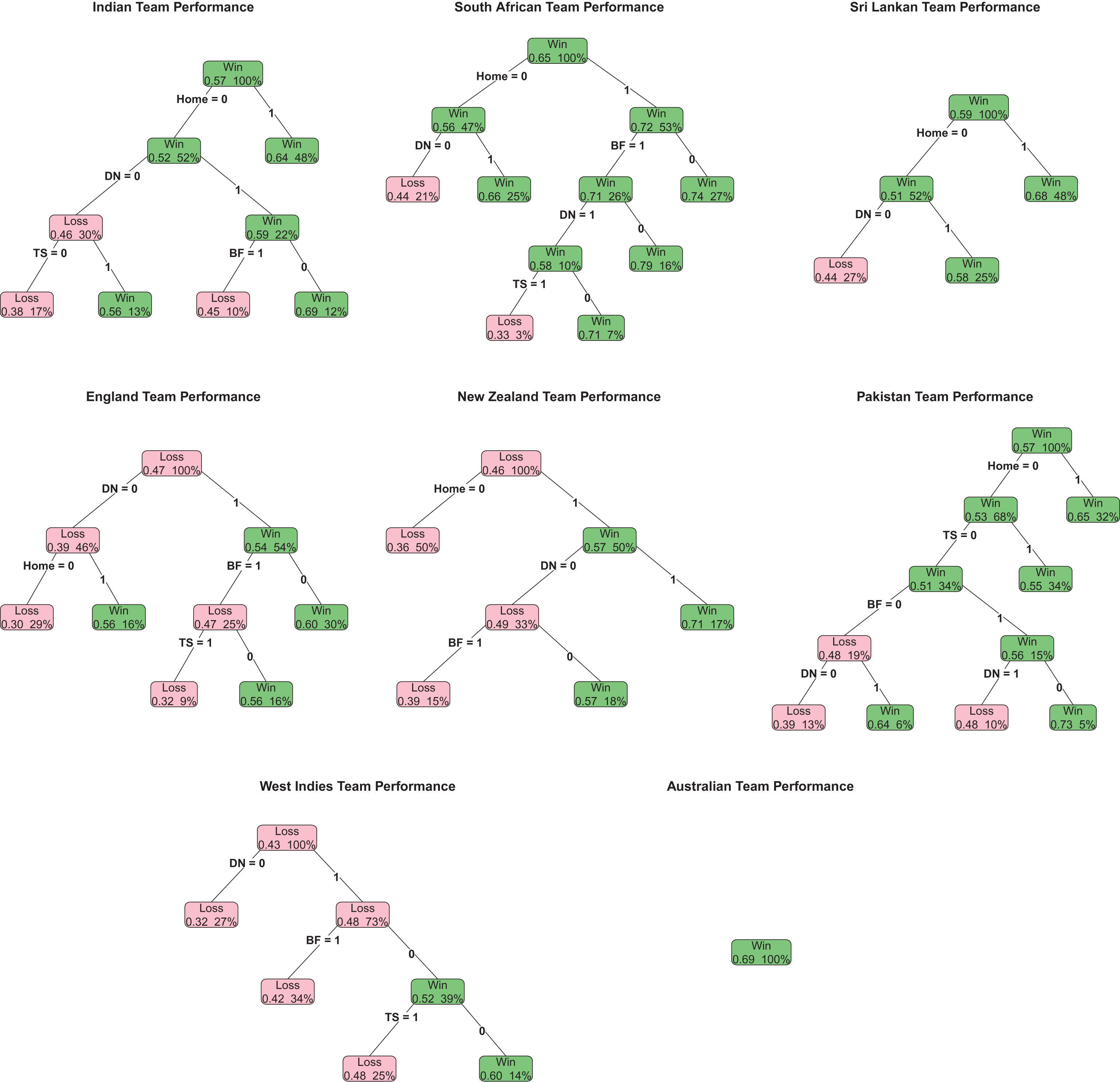
Fig.2
The model CT2 based classification trees for Indian, South African, Sri Lankan, England, New Zealand, Pakistan, West Indies and Australian Teams.
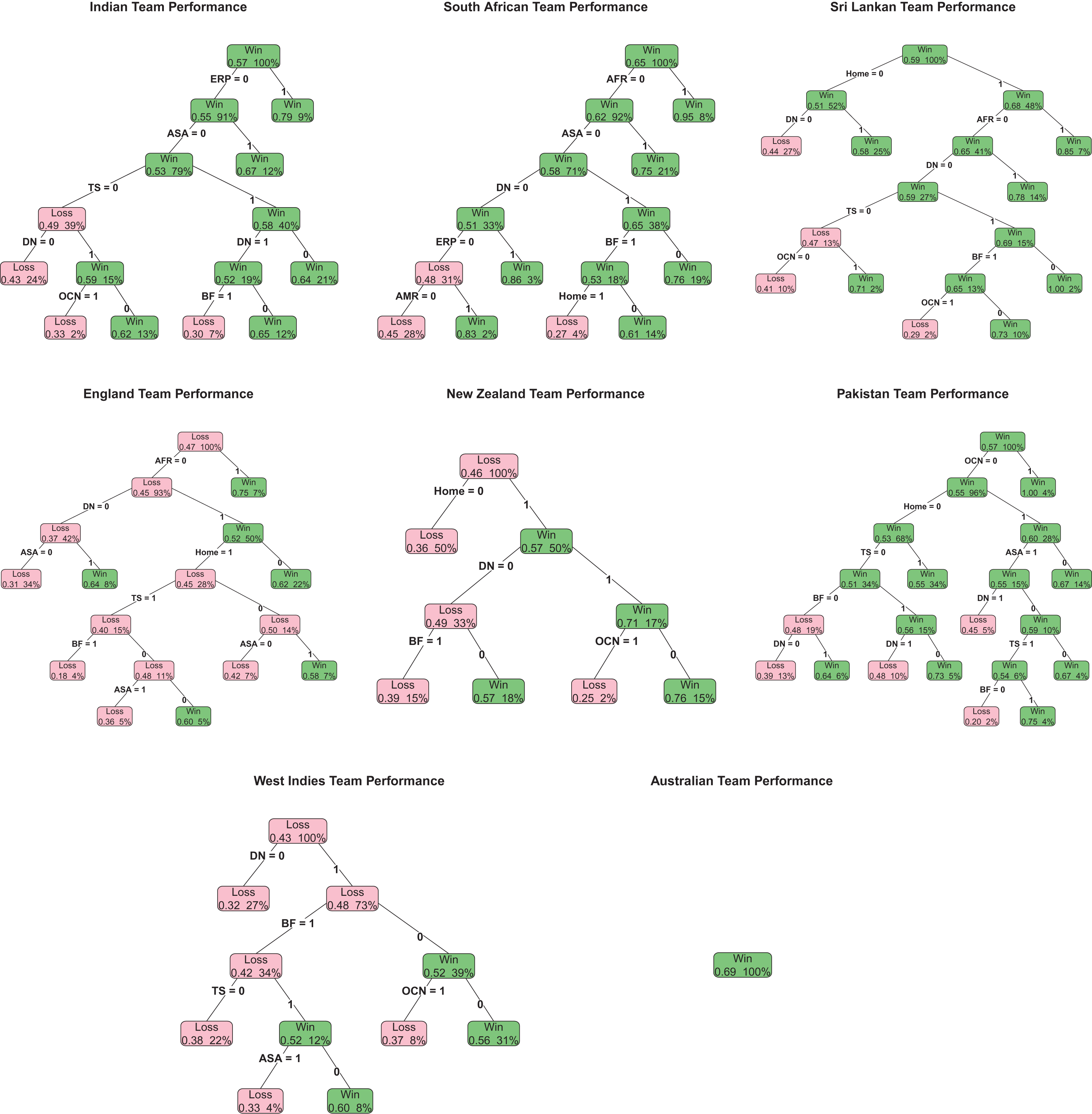
India: According to the model CT1, the home-field advantage is the primary factor for the Indian team as it is the root node of the tree structure. It is clear in the model CT2 that both the European and the Asian teams are large contributors to the India’s home-field advantage. When playing with teams from continents other than Asia and Europe, model CT2 indicates that winning the coin-toss is positively related to the outcomes of all games with worst case being loosing toss in a day-night games. In day only games, winning toss and batting second was successful for them. Losing toss against Oceanic opponents at home negatively impacted on the Indian team.
South Africa: Similar to the observations for the Indian Team, the home-field advantage is the primary node for the South African team in model CT1. The model CT2 indicates that the fellow African and the Asian teams are the primary victims of their success at the home venues. However, they have not had success in the day only home games when they batted first against the other nations. In day-night home games, they seem to be success against both American and European teams but the number of games played at those instances may not be sufficient to make strong conclusions. The model CT1 indicates that the South African team had more success in day only games than day-night games when they played away from home.
Sri Lanka: Both the models CT1 and CT2 indicate that the home-field advantage is the primary factor for Sri Lankan team success. Among the home games, they had a huge success against the African teams, but the coin-toss became significant when they played day-night games with the teams other than from Oceania and Africa. However, winning toss and batting first in day-night home games turned out to be a bad choice against the Oceanic teams. Both the models indicate that Sri Lanka had more losses in day-night away games.
England: As indicated in the logistic regression models, classification trees also indicate that the home-field advantage is not the primarily significant node for the England team. The home-field advantage is unconditionally significant when they played against African teams. The home conditions were positively impacted them when they played day-night games with Asian teams. They were more successful in the day only away games, but surprisingly the other factors such as coin-toss, batting first. and play with Asian teams appeared to have an impact on the day-only home games.
New Zealand: The home-field advantage is a significant factor for the New Zealand team. Just like the Sri Lankan team, both the models picked the home-field advantage as the root node for New Zealand. However, unlike any other teams, both models CT1 and CT2 provide very similar trees except that the model CT2 indicates that their performance in day-only games against the neighboring Australian team is vulnerable in the home conditions. It would not be a surprising fact given the Australians ability to adapt to New Zealand conditions far easily than any other country but the smaller number of games (2%) may not be sufficient to make a strong conclusion about this scenario. They had more victories in day-night games when they batted second at the home venues. Importantly, the coin-toss is not a part of their classifier list.
Pakistan: Like many teams, the Pakistan has also capitalized a significant home-field advantage. Unlike many countries, model CT2 indicates that they had a significant success against the Oceanic teams though they played only 4% of the home games against the these teams. Also, they had more successful day-night and less successful day only games against fellow Asian teams. The logistic model failed to capture this conditional behavior and simply indicated no significant Asian factor. In away games, winning the toss appears to have led to a higher wining percentage. However, losing toss in away games was critical for them because they won more game when batting first in day-night games and batting second in the day-only games and completely the opposite happened when they batted first in the day-only games and batted second in day-night games. Again, the logistic model fails to capture such conditional effects and the classification tree approach is far better in exploring such hidden behaviors.
West Indies: Just like the England team, the day-night game is the most important factor for the West Indies team. Surprisingly, the home-field advantage is not a part of either classification tree. Based on the model CT2, they had some successes in day-only games when they batted second against the teams except from the Oceania and batted first against non-Asian countries after winning the toss. However, model CT1 indicates that they failed to gain the advantage of the coin-toss win after elected to bat second in day only games.
Australia: None of the considered classifiers helped to obtain a meaningful classification tree for the Australian team. Their high winning rate in almost all the playing conditions make them less sensitive to the considered predictors. In the next section, we will discuss a possible extension of the current method to understand the Australian classifiers by considering their margin of the victories instead of the dichotomized win-loss in ODI games.
4Regression tree approach
In the classification tree approach, as well as in the logistic regression approach, the binary variable win-loss is used as the response variable. However, this variable loses some important information as the outcome of a match is simply dichotomized. For instance, this variable would not account for the margin of victory. Especially, in the situations where the dichotomized variable does not provide enough information to build successful decision trees, it may of value to consider alternatives such as the margin of victory as the response variable. As a result, one may need to adapt the regression tree approach in CART to build decision trees. We will use this approach to build interpretable decision trees for the Australian team.
Usually, the margin of victory is defined as the difference between scores of winning and losing teams. It would be a better variable than dichotomized response but it does not reflect some rare outcomes in ODI games such as rain interrupted matches where the difference does not reflect who won the match. Therefore, the difference in runs per over (average) is suggested to quantify the margin of victory by using properly adjusted batting averages. The adjusted batting average for the batting first team (AAvg1) is defined as
Instead of using the team’s scores, the defined adjusted averages are used to obtain the margin of victory (D). That is, D ij = AAvg i - AAvg j. Then the multiple regression model for the batting first team ‘i’ and batting second team ‘j’ is
(3)
where index ‘k’ represents the k-th repeat game between teams ‘i’ and ‘j’. It is assume that ɛijk ′s are identically and independently distributed normal random variables with mean zero and common standard deviation σ .
As in the logistic regression approach, we extend above model to incorporate the continent effect as follows,
(4)
One can adapt the regular multiple regression methods to identify the significance of the model parameters in the models (3) and (4). Instead, we directly apply these models in CART procedures to obtain the regression trees. The resulting regression trees for the Australian team are shown in Fig. 3. The green nodes on the regression trees indicate positive margin of victories (D > 0) favoring the Australian team and the percentage (%) indicates the number of matches (n) played under each condition as a percentage of the total number of matches they played.
Fig.3
The models (3) and (4) based regression trees for the Australian Team.
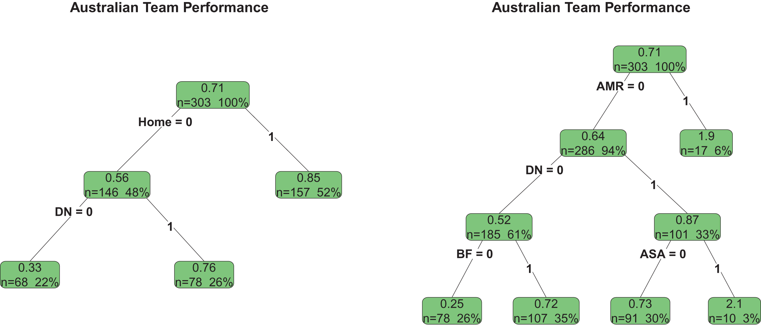
The regression trees indicate that how well the Australian team performed in almost all the conditions. One of their lowest margin of victories (D = 0.33) occurred when they played day-night games in the away venues. The Australian performance against the American teams is superior compared to the other teams, but the Asian opponents had the highest margin of loss to Australia when they played day only games in Australia. Batting first provided better margin of victory for the Australians when the game is day-night and played with opponents other than American teams. The coin-toss had no significant effect on their margin of victories.
5Discussion
In this study, we discussed the popular logistic regression model to identify the significance of ODI cricket predictors. Subsequently, we investigated the effects of those predictors considering day and day-night games separately. We provided a CART based alternative modeling strategy to model outcomes of ODI cricket matches that allows identifying important predictors in a practically interpretable way. Further, we extended that model by incorporating a modified version of margin of victory as the response instead of the classic dichotomous win/loss classification. This model allows us to extract important information about the game outcomes such as for the Australian team when the dichotomous variable was less informative. Also, the inclusion of continent factor in both logistic regression and CART models allows us to estimate the home-field advantages based on the opponent geographical location and helps getting a deeper understanding of the role of these predictors in the final outcome of the game.
Home-field advantage was found to be significant for many teams including India, South Africa, Sri Lanka, New Zealand, and Pakistan. Among all the teams, the South African team has the highest winning chance (72%) in home games. Australian team shows a higher margin of victory for home games compared to away games. We do have strong evidence to conclude that the West Indies team has no significant home-field advantage. One can consider West Indies as a neutral venue for world class tournaments such as the ICC Cricket World Cup.
Acknowledgments
The authors thank the anonymous referees and the editor for their useful comments and suggestions on an earlier version of this manuscript which resulted in this improved version.
References
1 | Allsopp P. , (2005) . Measuring team performance and modelling the home advantage effect in cricket, Unpublished PhD thesis, p. 149. |
2 | Bandulasiri A. , (2008) . Predicting the winner in one day international cricket, Journal of Mathematical Sciences & Mathematics Education 3: , 6–17. |
3 | Belson W.A. , (1959) . Matching and prediction on the principle of biological classification, Applied Statistics, 65–75. |
4 | Breiman L. , Friedman J. , Stone C.J. and Olshen R.A. , (1984) . Classification and regression trees, CRC press. |
5 | Clarke S.R. and Norman J.M. , (1995) . Home ground advantage of individual clubs in english soccer, The Statistician, pp. 509–521. |
6 | CricInfo, (2015) . Espncricinfo (formerly cricinfo) is a sports news website exclusively for the game of cricket. www.espncricinfo.com |
7 | De Silva B.M. and Swartz T.B. , (1998) . Winning the coin toss and the home team advantage in one-day international cricket matches, Department of Statistics and Operations Research, Royal Melbourne Institute of Technology. |
8 | Elderton W. and Wood G.H. , (1945) . Cricket scores and some skew correlation distributions:(an arithmetical study, Journal of the Royal Statistical Society, 1–11. |
9 | Fernando M. , Manage A. and Scariano S. , (2013) . Is the home-field advantage in limited overs one-day international cricket only for day matches? South African Statistical Journal 47: , 1–13. |
10 | Fielding A. and O’Muircheartaigh C. , (1977) . Binary segmentation in survey analysis with particular reference to aid, The Statistician, 17–28. |
11 | Harville D.A. and Smith M.H. , (1994) . The home-court advantage: How large is it, and does it vary from team to team? The American Statistician 48: , 22–28. |
12 | Hoult N. , (2016) . English cricket braced for revolution as toss is scrapped in county championshi. http://www.telegraph.co.uk/cricket/2016/04/09/english-cricket-braced-for-revolution-as-toss-is-scrapped-in-cou/ |
13 | Karlis D. and Ntzoufras I. , (1998) . Statistical modelling for soccer games: the greek league, Department of Statistics (Athens University of Economics and Business, Greece). |
14 | Levernier W. and Barilla A.G. , ((2007) ): “An analysis of the home-field advantage in major league baseball using logit models: Evidence from the 2004 and 2005 seasons,”, Journal of Quantitative Analysis in Sports, 3. |
15 | Mather V. , (2015) . Coin toss retains its place in history, if notin cricket. http://www.nytimes.com/2015/12/01/sports/international/coin-toss-is-secure-in-sports-lore-if-not-in-cricket.html?_r=. |
16 | Messenger R. and Mandell L. , (1972) . A modal search technique for predictive nominal scale multivariate analysis, Journal of the American Statistical Association 67: , 768–772. |
17 | Morgan J.N. and Messenger R.C. , 1973. Thaid: A sequential analysis program for the analysis of nominal scale dependent variables. |
18 | Morgan J.N. and Sonquist J.A. , (1963) . Problems in the analysis of survey data, and a proposal, Journal of the American Statistical Association 58: , 415–434. |
19 | Pollard R. and Gómez M.A. , (2014) . Comparison of home advantage in men’s and women’s football leagues in europe, European Journal of Sport Science 14: , S77–S83. |
20 | R Core Team, (2012) . R: A Language and Environment for Statistical Computing, R Foundation for Statistical Computing, Vienna, Austria, URL http://www.R-project.org/, ISBN 3-900051-07-0. |
21 | Ribeiro H.V. , Mukherjee S. and Zeng X.H.T. , (2016) . The advantage of playing home in nba: Microscopic, team-specific and evolving features, PloS One 11: , e0152440. |
22 | Silva R.M. , Manage A.B. and Swartz T.B. , (2015) . A study of the powerplay in one-day cricket, European Journal of Operational Research 244: , 931–938. |
23 | Therneau T. , Atkinson B. , Ripley B. and Ripley M.B. , (2015) . “Package rpart,”. |
24 | Vaz L. , Carreras D. and Kraak W. , (2012) . Analysis of the effect of alternating home and away field advantage during the six nations rugby championship, International Journal of Performance Analysis in Sport 12: , 593–607. |


