
A flight-based metric for evaluating NFL punters
Abstract
Common evaluation metrics for NFL punters are outdated, failing to account for field position and touchbacks. Using detailed information on each punt of the 2013 season, a nonlinear model is developed, using these factors alongside hang time, coverage quality, and environmental conditions. This leads to punter evaluation metrics using expected points added (EPA), both in total and per punt. The persistence of punting skill is explored, and the relationships between performance and salary are discussed.
1Introduction
1.1Player evaluation in American football
Direct metrics for player evaluation are more difficult to construct in football than in some other sports, due to the interconnectedness of players’ responsibilities. In baseball, a double to left-centerfield can be credited solely to the batter, with blame falling solely on the pitcher. A three-point basket likewise involves only the shooter, the defender, and perhaps a passer or screener. In contrast, an eight-yard rushing play in football might directly involve over half of the players on the field, raising a challenging issue of how to distribute credit appropriately. In soccer and ice hockey, metrics are still more difficult to formulate, due to these sports’ continuous nature and the relative infrequency of scoring plays (Gerrard, 2007). However, some actions in American football have a substantial degree of independence, notably passing and kicking, allowing for more straight-forward assessment of the contributions of quarterbacks, kickers, and punters.
Traditional quarterback metrics such as the decades-old NFL Passer Rating (see NFL, 2016) rely solely on readily countable items – completions, attempts, touchdowns, interceptions, and yards gained. Contemporary metrics include the sum of expected points added (EPA) or win probability added (WPA) on passing plays, the computation of which require knowledge of the game situation before each play, including down, distance, line of scrimmage, and (for WPA) score; see Burke (2014a) and Burke (2014b) for background on these. The popular Total Quarterback Rating (QBR) used by ESPN (see Oliver, 2011) requires subjective analysis of items beyond the play-by-play account.
Field goal kickers are frequently evaluated in the mainstream media by the number of kicks made and/or the percentage successful, both of which ignore the lengths of kick attempts. Models that include distance have been around for decades, such as Berry & Berry (1985) and Morrison & Kalwani (1993), and an early study including weather and game situation (Bilder & Loughin, 1998) was published shortly after play-by-play game accounts became widely available. More recent models, notably Clark et al. (2013) and Pasteur & Cunningham-Rhoads (2014), use multiple seasons of data to estimate a generic kicker’s success probability for each kick attempt, incorporating the distance, surface, environmental conditions, and game situation, then compare individual kickers’ aggregate performances to the model. This approach naturally leads to EPA values for each kicker, on either in total or per kick, the former allowing for easy comparison with the impact of players at other positions.
1.2Existing punter performance metrics
While a field goal attempt has a binary outcome, a range of results is possible for a punt, increasing the potential scope of metrics. The simplest is gross distance, the number of yards downfield beyond the line of scrimmage the ball travels before rolling to a stop, leaving the field of play, or being picked up by a member of either team. Note that this excludes the distance from the punter to the line of scrimmage, so the ball travels approximately 15 yards farther downfield than the gross punting value indicates. Net distance is conceptually similar to gross distance, but subtracts out any return yardage by a receiving player who fields the ball. A touchback, in which the ball lands in or bounces into the end zone and is subsequently placed at the receiving team’s 20-yard-line, is typically undesirable for a punter, and the percentage of punts resulting in touchbacks is another possible metric. In most cases, a punt that results in the receiving team starting from inside their own 20 is viewed as successful for the punting team, and the number of inside-20 punts by a player is routinely tabulated. Finally, while not included in the official play-by-play statistics, the hang time that a punt stays in the air, is often referenced in television broadcasts. A longer-than-average hang time gives the punter’s teammates more time to get downfield before the ball lands, possibly reducing return opportunities, thus increasing net punting distance. In contrast, a low “line drive” punt with a shorter hang time may allow a returner to catch the ball and accelerate to full speed before defenders get in position to tackle him, increasing the chance for a long return.
Unfortunately, the aforementioned metrics are hampered by confounding variables. If the line of scrimmage is near midfield, then often the punter will reduce the amount of power behind a kick, in order to avoid a touchback, leading to a reduced gross (and likely also net) distance, as discussed in Burke (2010). If a punt originates from deep in the kicking team’s own end of the field, there are no such concerns about a touchback, so the punter is free to kick the ball as far as possible. Punters on weak teams more often find themselves with plenty of room to kick the ball deep, leading to higher gross punting averages and fewer touchbacks. Lisk (2008) found that punters on teams with below-average offenses are overrepresented on Pro Bowl (all-star) teams, perhaps for this reason. On the other hand, punters on good teams can expect to have higher inside-20 percentages, because of having more frequent short-field punt opportunities.
An unrelated issue is that good punt coverage inhibits long returns, leading to an increase in net yardage, and may also reduce touchbacks, even though neither of these effects are caused by the punter. Additionally, NFL statistical guidelines credit a punter with net yardage all the way to the goal line on a touchback, rather than reducing it by 20 yards. To illustrate this, consider two punts, both with a midfield line of scrimmage. The first punt is caught on the fly at the 10-yard line and returned to the 15; the punter has gained 35 yards of field position for his team, and is credited with 40 gross yards and 35 net yards. A second punt lands in the end zone and is not returned; the line of scrimmage will be the 20, so the punter has advanced the ball only 30 yards, but is credited with 50 yards gross and 50 yards net distance. The first is clearly a better result, and this is reflected in the touchback and inside-20 statistics, but net distance (which is more commonly referenced) gives less credit to the better outcome. Finally, a punt which is blocked and remains behind the line of scrimmage is not considered a punt at all for statistical purposes, but one that is partially blocked and flies or rolls beyond the line of scrimmage is counted (typically with very poor gross and net distances.) Blocked and partially blocked punts can occur through the fault of the punter, snapper, and/or blockers, and more information would be required to properly appropriate blame for these mishaps.
Using data from the 2000– 2009 seasons, Burke (2010) generated a model that accounted for field position, leading to metrics of expected points added per punt and total win probability added. Other models that include field position (Tymins, 2014; Beuoy, 2012) used multiple seasons of data to document the improvement of punters in recent years, to look more carefully at touchbacks, and to give some insight into the economic value of punters.
2The influence of field position
2.1Five seasons of punts
We began our investigation by considering the 12,245 regular-season punts from the 2010– 2014 seasons, using data from the online Game Play Finder tool at Pro Football Reference (http://www.pro-football-reference.com/play-index/play_finder.cgi). Figure 1 shows the average gross, net, and effective net (adjusted for touchbacks) punt distances, by field position. The average gross distance is relatively constant for punts taken more than roughly 60 yards from the end zone, meaning that concerns over touchbacks start to become a significant issue when the line of scrimmage is beyond the punting team’s 40-yard line. As the available field becomes shorter, the gross distance drops nearly linearly, but with a slope less than one, so additional field position gained beyond the 40 is still somewhat advantageous to the punting team. The curve for effective net distance has a similar shape, but is a bit more rounded, as opposed to nearly piecewise linear. In contrast, net distance has an odd peak related to touchbacks, with the difference between the net and effective net curves directly reflecting touchback frequency.
Fig.1
Gross, net, and effective net punt averages by field position, 2010– 2014.
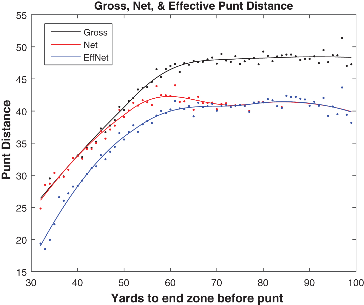
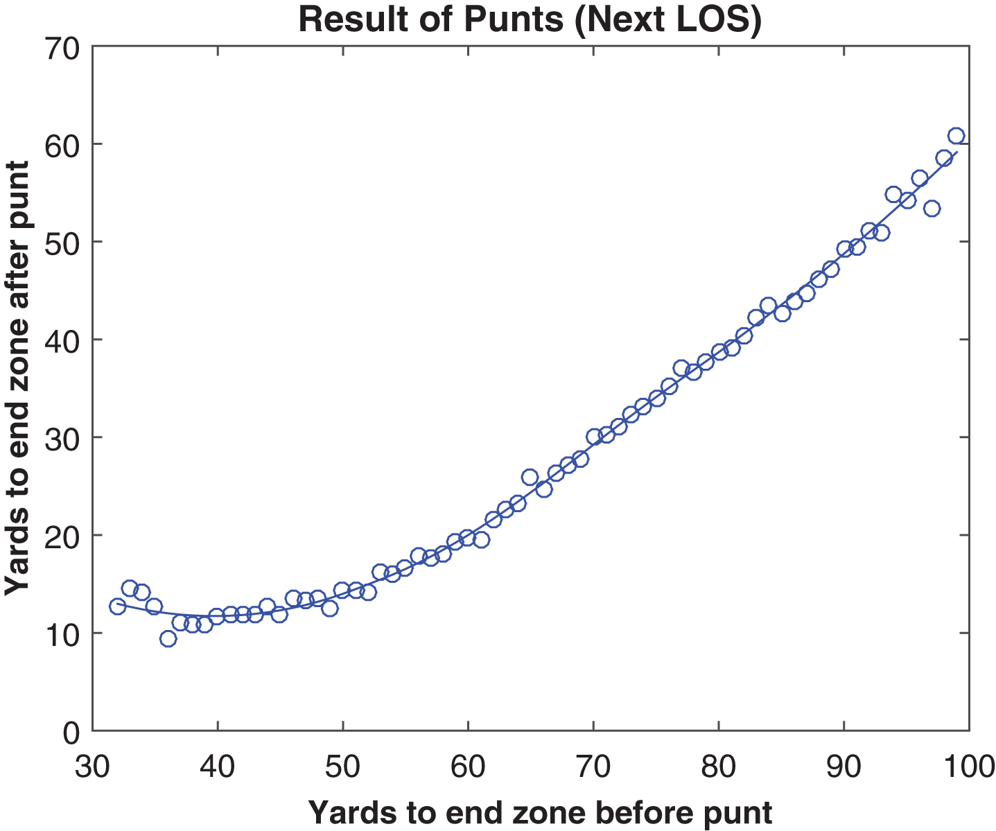
The difference between the gross and effective net curves (both LOESS-smoothed) in Fig. 1 can be interpreted as the change in field position between the ending point of a punt and the next line of scrimmage, a change which occurs through touchbacks and returns. Figures 2 and 3 show the probability of a touchback and the expected return distance, both by field position. Touchbacks are principally an issue on short-field punts, and returns are more a concern on long-field punts; when the line of scrimmage is between roughly the kicking team’s 35 and 45, touchbacks and returns are about equally important. Differences in expected return distance occur mostly due to the probability of a positive return; the average lengths of returns are relatively stable across field position. Reframing the information from Fig. 1, Fig. 4 shows the average outcomes of punts, as measured by the next line of scrimmage, after the punt. We can observe that in a punting situation, there is minimal benefit retained from any yardage gained beyond midfield before the punt, as the expected next line of scrimmage is about the same regardless of the point in the opponent’s territory from which the punt occurs.
Fig.2
Touchback probability by field position, 2010– 2014.
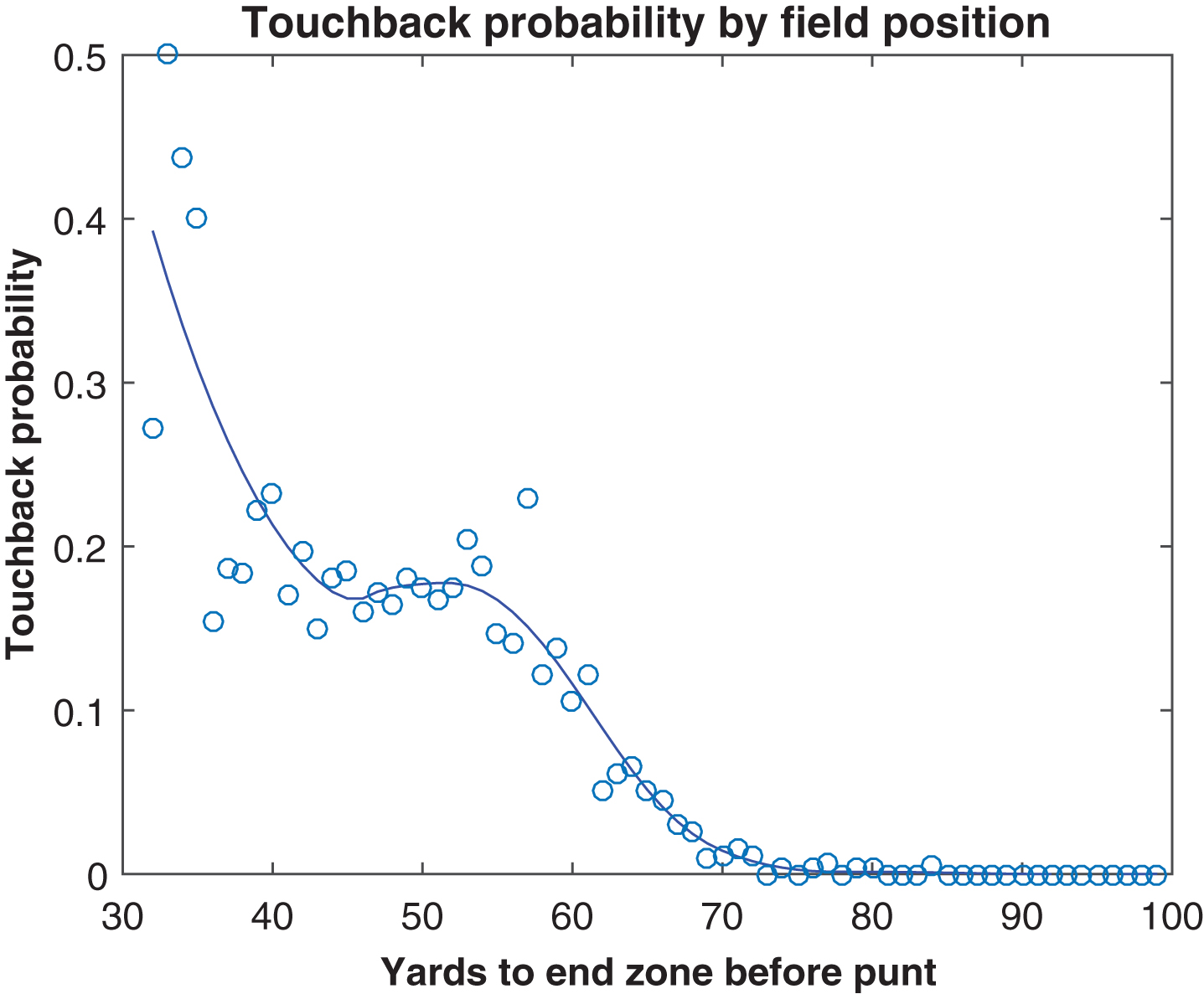
Fig.3
Expected return distance, by field position, 2010– 2014.
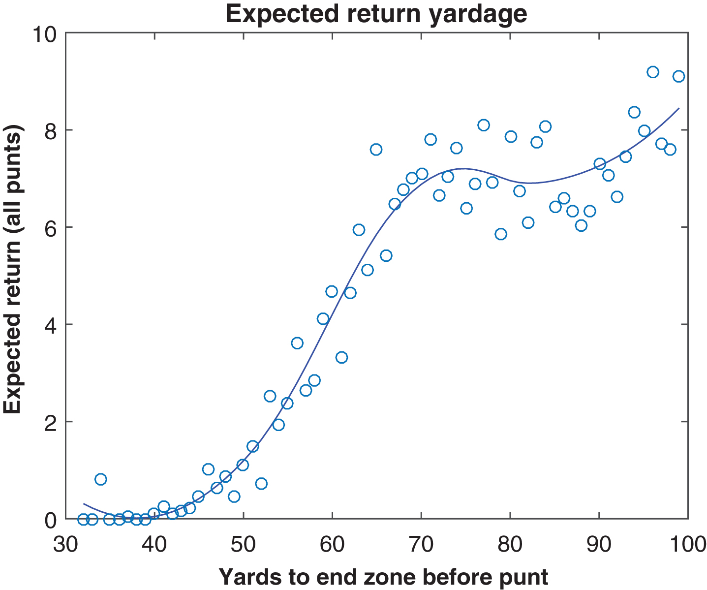
Fig.4
Next line of scrimmage by field position, 2010– 14.
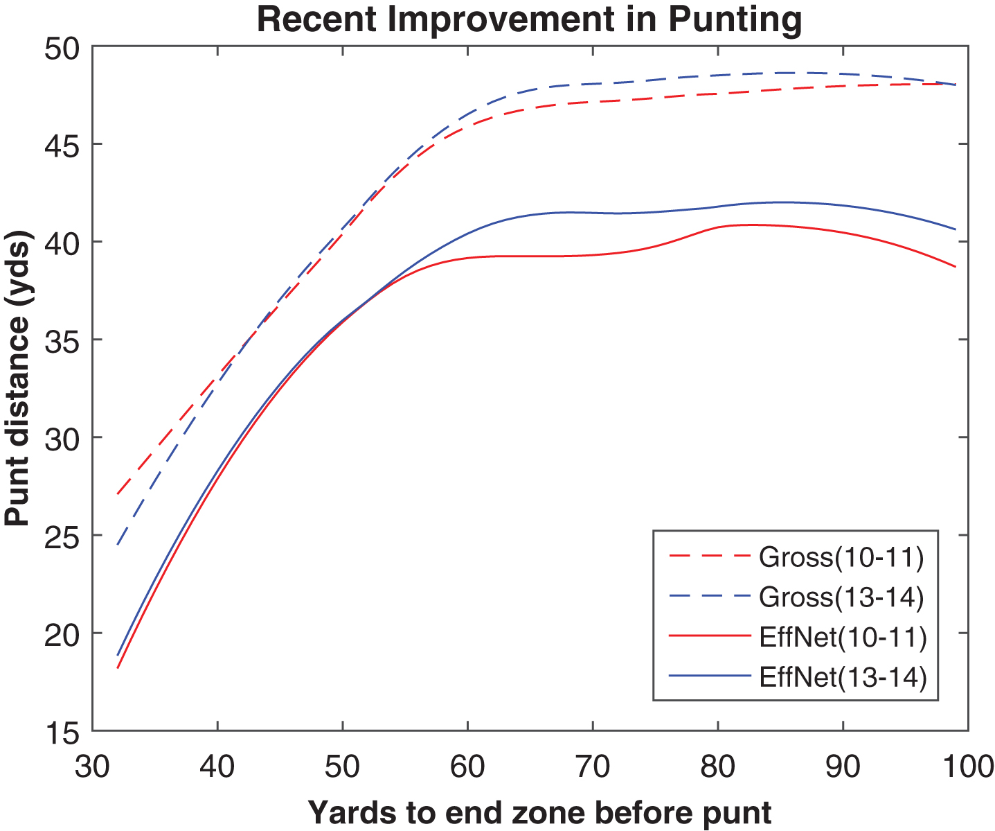
Confirming the findings of Beuoy (2012) with newer data, we see continued improvement of punters in recent years. Figure 5 compares the gross and effective net punting distances, across field position, in 2010-11 versus 2013-14, and we see improvement of about one yard on long-field punts. Interestingly, the differences are larger in effective net distance than gross distance. While this could relate to coverage quality, it could also occur due to an increased punt hang time at a given distance, allowing the coverage more time to get downfield, but we have no data from which to explore this hypothesis.
Fig.5
Gross and effective net punting by field position, 2010-11 and 2013-14.
2.2A new approach
The punter’s influence on a play is largely confined to the kick itself, as punters are rarely good tacklers. With this in mind, punters could be evaluated based on the landing point of the ball, after accounting for field position. Under such a paradigm, downfield flight distance is the key measure, and touchback probabilities, returns, roll distance, penalties, and turnovers must be modeled. This paradigm reduces the confounding effects of coverage and returner quality, and the randomness inherent in long returns. However, data on punt flight distance is not published by the NFL.
To collect such a data set, we subscribed to the NFL’s online video service, which allows access to archived play-by-play video of games from previous seasons. For each of the 2,526 punts during the 2013 regular season, with the exception of the 16 blocked punts, we collected data on the landing point and eventual end point of each punt (visually estimating to the nearest yard, both downfield and laterally). Also from video, we estimated hang time (by hand via stopwatch, taking the mean of three measurements). We also aggregated hourly weather data for each game, using the game-time weather for first quarter punts, and one hour later with each subsequent quarter. Noting the direction of each punt relative to the home team’s bench, and determining stadium orientation via Google Maps and the location of the home bench on seating diagrams, we were able to estimate the direction (on a 16-point compass rose) of a punt. This allowed for decomposing wind speed into a headwind/tailwind component (differentiating between the two) and a crosswind component, via trigonometry.
The play-by-play text from Pro Football Reference lists returns as they occurred on the field, before enforcement of any penalties. However, most penalties against the return team are enforced at the spot of the foul, often negating some or all return yardage on the play, so additional work was required to ascertain the adjusted return yardage. By looking at the line of scrimmage for the next play, we could determine where a penalty was enforced, and reduce the return yardage accordingly, when necessary, as would be done for official statistical records.
Among the 2510 punts in our data set, there were 257 with an enforced penalty. Over 70% of these penalties were against the return team, with an average of 9.3 penalty yards assessed; most were for holding or an illegal block, each of which is a 10-yard foul except when that would be more than half the distance to the goal line. Just over a third of return team penalties also included a reduction (or complete elimination) of return yardage, with an average of 18.1 yards lost, as the advantage gained often led to long returns. Penalties against the punting team averaged 11.5 yards, with a variety of foul types notably including offensive holding before the punt (10 yards), face mask (15), fair catch interference (15), and illegal formation (5). On a per-punt basis, we observed an average of 0.32 penalty yards against the punting team, 0.69 yards against the receiving team, and 0.49 yards of negated returns, for a net effect of 0.86 yards per punt against the return team. In the remainder of the manuscript, all 2013 return yardage numbers have been adjusted for the impact of penalties.
2.3Fly distance and landing point
Fig.6
Punt fly distance and other measures, 2013.
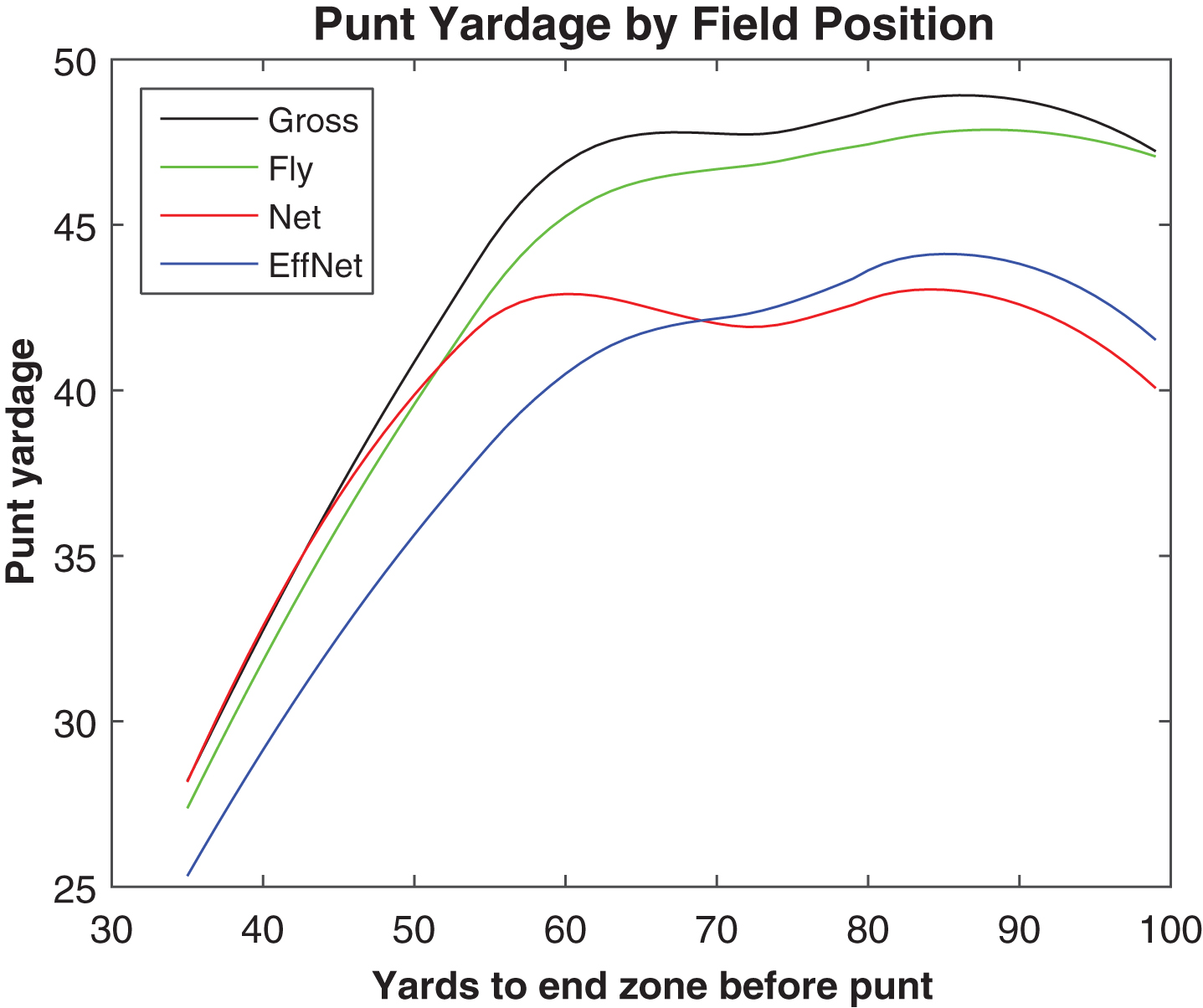
On punts that land in the end zone or out-of-bounds, flight distance and gross distance are the same, and this is true for those caught on the fly, as well. However, on punts that bounce within the field of play, they may differ. Punt fly distance is about a yard less than gross distance on average, as shown in Fig. 6, with the extra yard representing downfield roll. On long-field punts where a touchback is unlikely, the difference between net and effective net comes from the receiving team being penalized more frequently on such punts.
Figure 7 breaks down the field position change after landing into its components (roll, return, touchbacks, and penalties), by field position. Despite the higher rate of touchbacks in short-field situations, the average total “return” distance after a punt lands is far less in such cases than in long-field situations. It is notable that while punt return distance is roughly the same when the line of scrimmage is anywhere between the punt team’s 10 and 30 yard line (i.e. 70– 90 yards from the far end zone), returns are significantly greater when the punt team is backed up near its own goal line. While the sample size is too small to draw clear conclusions, this seems plausible, as the punter is closer to the line of scrimmage in such situations, perhaps forcing his team to focus on avoiding a blocked punt, delaying the chance to get downfield.
Fig.7
Composition of post-bounce yardage by field position, 2013.
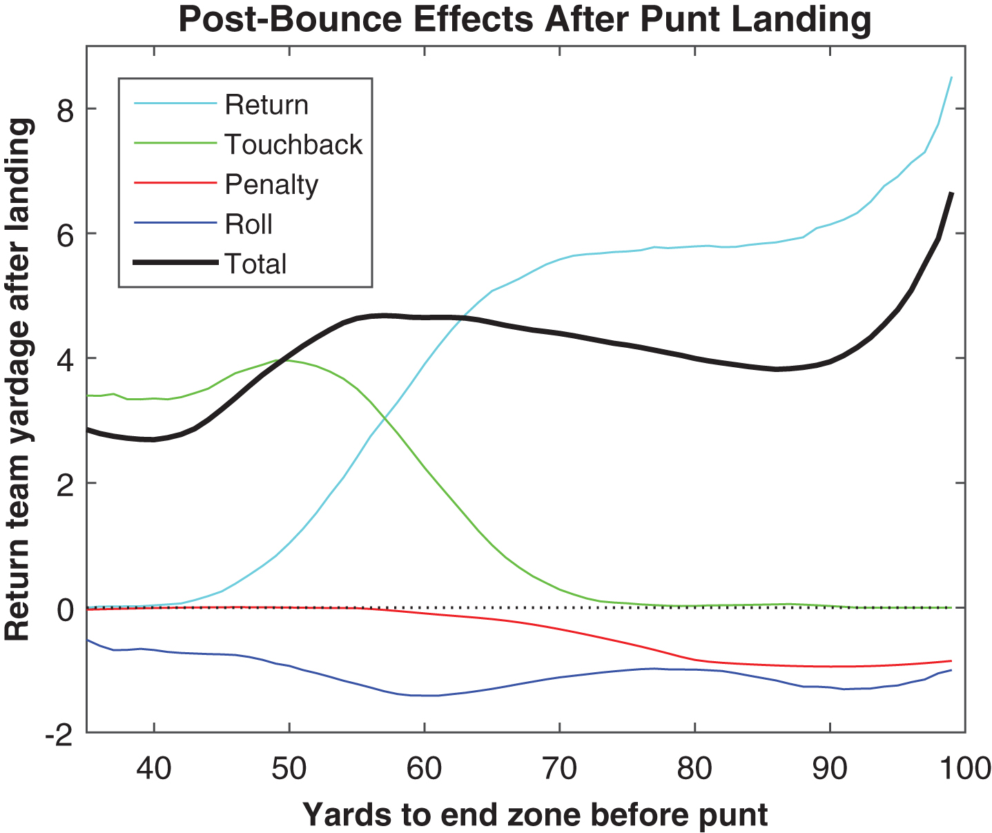
Fig.8
Punt bounce probability by landing point, 2013.
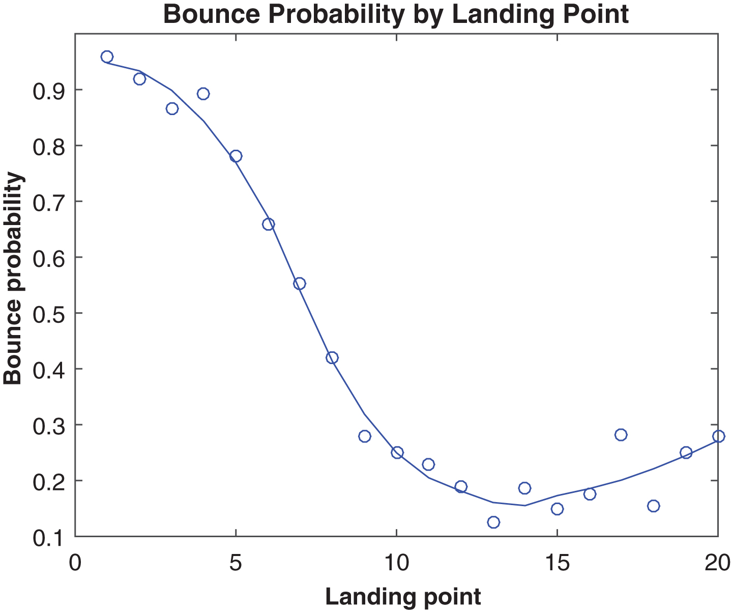
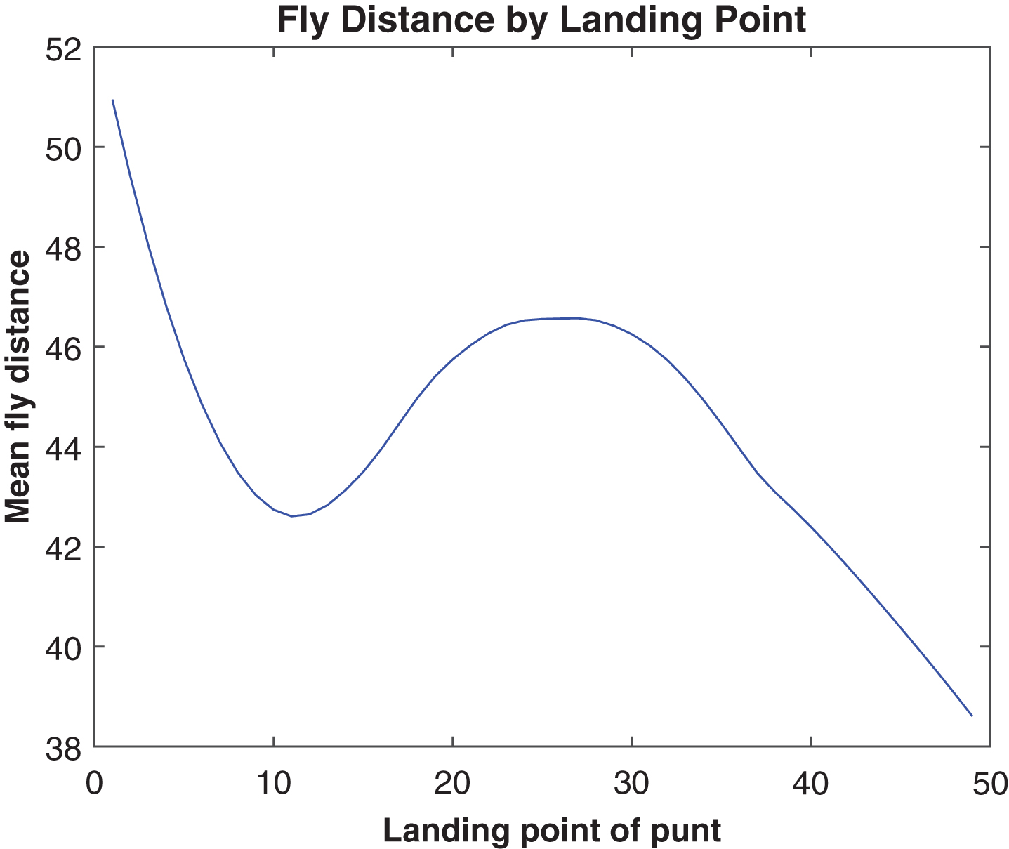
The location at which a punt lands has a strong influence on how the remainder of the play unfolds. Figure 8 shows that the probability of a punt being allowed to bounce (after landing in-bounds) drops precipitously between the 5 and 10 yard lines. This seems to be in line with a traditional short-field punt return strategy of the returner standing at his 10-yard line, and avoiding the ball if it flies over his head, anticipating a touchback. Indeed, Fig. 9 shows that a touchback is three times more likely on a punt landing at the 5-yard line than on one landing at the 10. In considering the next line of scrimmage, Fig. 10 shows that punts landing between the 5 and 10 have the best outcomes. Interestingly, punts landing very near the end zone tend to be long punts, and those landing between the 10 and 15 tend to be short, as shown in Fig. 11, possibly indicating that these were over- and under-kicked, respectively.
Fig.9
Touchback probability by landing point, 2013.
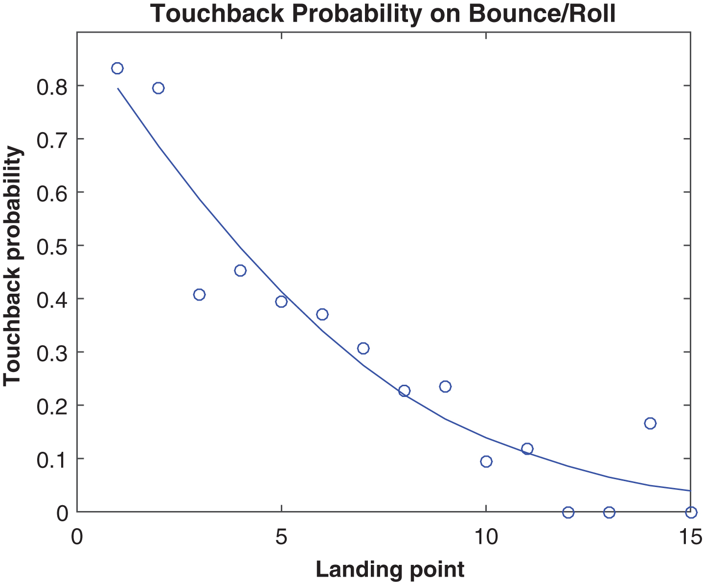
Fig.10
Next line of scrimmage and net “return” after landing, 2013.
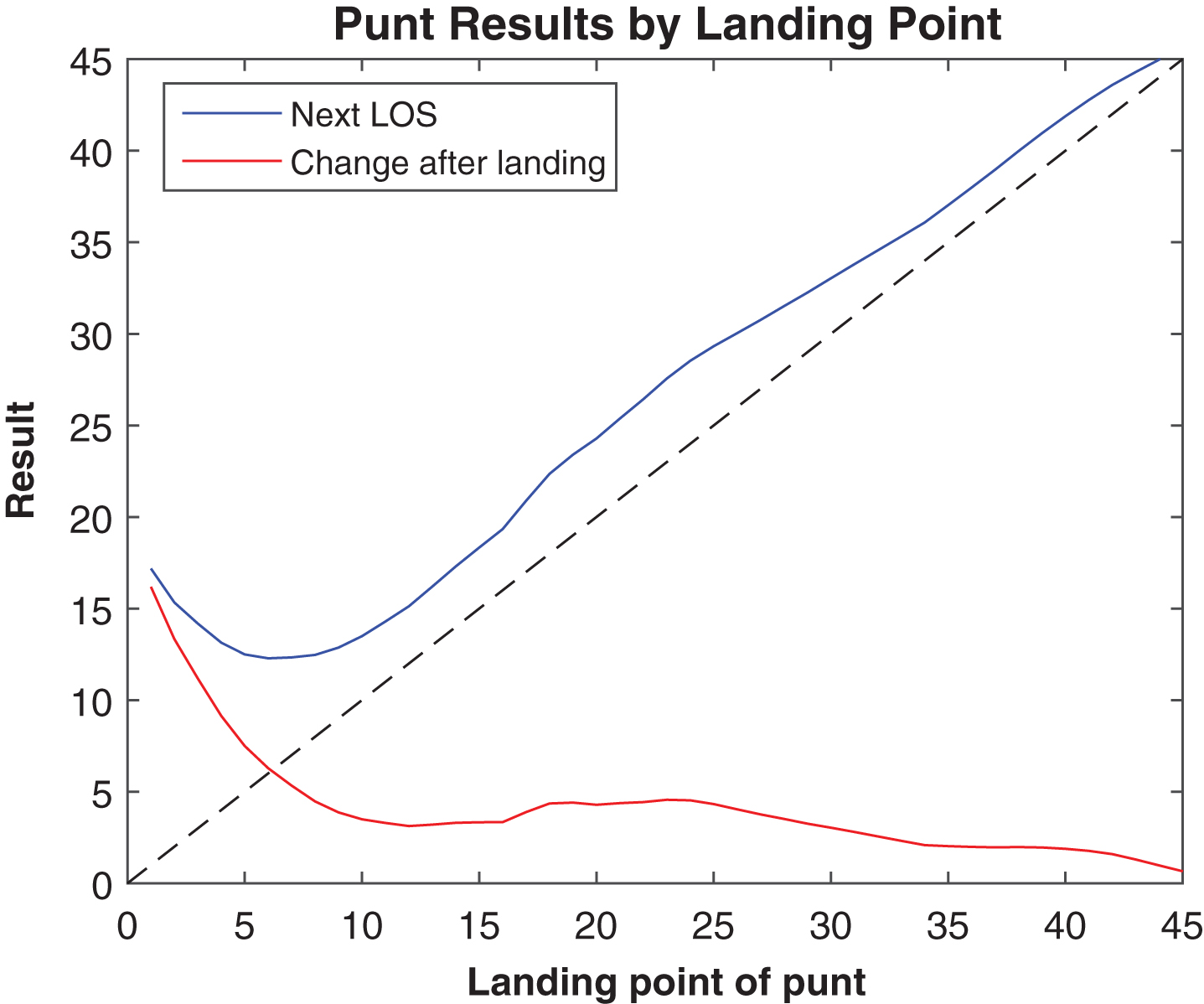
Fig.11
Average fly distance by landing point, 2013.
Based on the above, it seems possible to create a punter metric by subtracting the expected post-bounce adjustment based on the landing point (from Fig. 7) from the actual fly yardage, then compare this to the average effective net yardage (from Fig. 6). Aggregating these values for each punter leads to expected yards added (EYA), and EYA per punt.
Fig.12
Average post-bounce “returns” by landing point and fly distance, 2013.
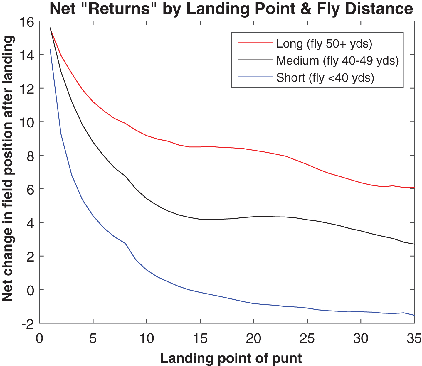
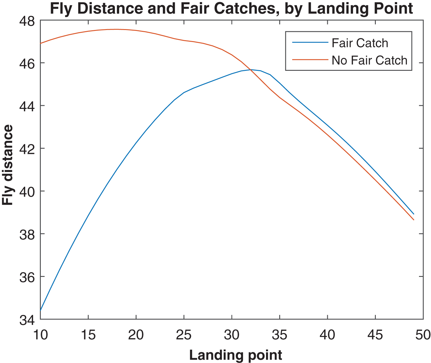
However, a key shortcoming of this model is that subsequent occurrences after a punt lands depend not only on where it landed, but also on how far it flew to get there. Figure 12 shows that, at any given landing point, longer punts have inferior post-bounce outcomes to shorter ones, presumably because of the additional distance the coverage must run to be in position to make a tackle. This is not to say that kicking the ball farther is undesirable, but only that some of the extra punt distance will be negated by longer returns. Part of this effect is explained by Fig. 13, in which we see that punts resulting in fair catches tend to have shorter flight distances, at least for punts landing inside the 30.
Fig.13
Average fly distance for punts resulting in a fair catch or not, by landing point, 2013.
Given that not every yard of field position is equally valuable, but rather those yards near the goal lines are worth more, as discussed in Romer (2006) and Burke (2008), the preferred unit of measure for punter value is expected points added (EPA). EPA can be computed in total or averaged per punt, starting from a table of EP values at each yard line; we generated such a table from the graph in Burke (2014a). EPA is a common unit that allows readily for comparisons among players at different positions, and it allows us to account for the value associated with turnovers. There were 81 fumbles by the receiving team in 2013, of which 63 occurred while attempting to catch the ball, with the remainder happening during returns. Receiving teams recovered their own fumbles two-thirds of the time, but 27 were recovered by the punting team.
3Multi-factor models
3.1Modeling post-bounce effects
Fig.14
Expected next line of scrimmage, by landing point and fly distance, 2013.
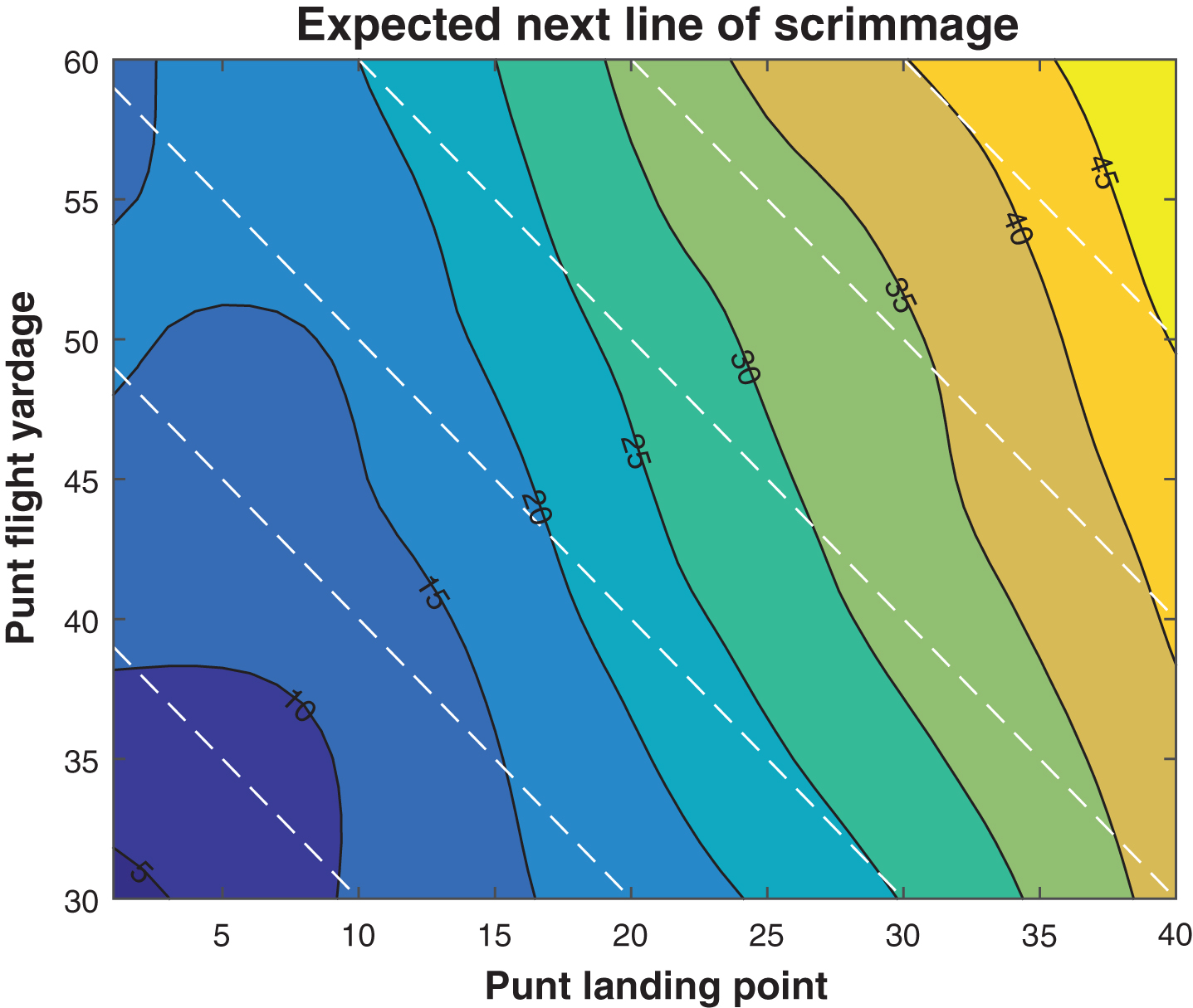
To generate a model for post-bounce net yardage with two independent variables, landing point and fly distance, we apply a modified ridge estimator (d’Errico, 2005) to smooth the empirical data. This allows for modeling the resulting next line of scrimmage, a contour plot of which is shown in Fig. 14. On this plot, all points on a given dashed white line represent the same pre-punt field position. As we move up and left along a dashed line, the length of the punt increases (so the landing point yard-line decreases.) If the colored contour lines were parallel to the dashed white lines, this would indicate a zero net benefit to longer punts, in that the additional flight distance would be completely offset by longer returns. On the other hand, if the contour lines were vertical, then the expected line of scrimmage would be based solely on the landing point, independent of the flight distance. However, except in the left portion of the graph (where touchback effects are dominant), we observe that the contour lines are oriented neither vertically nor parallel to the dashed lines, but somewhere in between. Based on the slopes, we see that each extra yard of flight distance increases the expected punt return by about a half-yard, with the remaining half-yard being a net gain in field position.
From the pre-punt field position and actual fly distance, we can use the above model to determine the expected next line of scrimmage for a punt, removing coverage quality as a confounding variable and reducing randomness. If we compare this modeled result to expected effective net yardage based solely on field position, then we have a metric for expected yards added on that punt, i.e. EYA = actual downfield flight – (modeled post-bounce “return” + expected effective net distance). We can obtain an EPA model similarly, replacing distances by their associated changes in expected points (dependent not only on how many yards of field position, but also where on the field those changes occur).
We then seek to improve this model by considering factors in the control of the punter, namely the lateral landing point (measured by edge distance, the number of yards from the landing point to the nearest sideline) and the hang time. We first consider correlations between these factors and the residuals of the above model, on punts landing in particular regions (by yard-line), then use a two-fold cross validation procedure (Picard & Cook, 1984) with 10,000 repetitions to see which factors are predictive in various situations. Long-field punts and short-field punts often involve different kinds of kicking techniques, so we consider these cases separately. In experimenting with various thresholds for defining long-field punts, we found that including those where a touchback would require a punt of 60+ yards (i.e. the line of scrimmage is at or inside the punting team’s 40-yard-line) gave the most meaningful results.
Hang time is a predictive factor only on long-field punts landing in-bounds between the 10-yard-line and 30-yard-line, and the fit adjustment to EPA is 0.180 · hangtime – 0.798, with the constant term ensuring a mean value of zero across all punts. Comparing the hang time coefficient to the 0.557 EP change associated with yard of field position away from the end zones, we find that an extra second of hang time is worth just over three yards. We tested models that used hang time relative to expectations for the fly distance and/or landing point, since both are in the EPA model, but the results were quite similar, so we opted for simplicity.
Traditional wisdom holds that landing the ball just inside the sideline can be valuable, by helping limit return yardage. On punts landing near the goal line, this is thought to help prevent touchbacks, as the ball may bounce out of bounds before crossing the goal line. We could not find sufficient evidence of predictive value to include this factor in our model. However, it warrants further exploration, as our sample sizes of such punts (especially those landing near the corner of the goal line and sideline) are relatively small and there is quite a bit of randomness involved in the outcomes.
3.2Additional factors
Other factors not in the punter’s control, such as environmental conditions and coverage quality, may also be significant. For short-field punts, none of the factors considered substantially reduced predictive error in our cross validation tests. However, for long-field punts, multiple factors were individually predictive, and the greatest error reduction occurred with the combination of temperature, a binary variable for precipitation, and coverage quality. We used DefPPG, the number of points per game allowed by the punting team’s defense, as a proxy for punt coverage quality. The coefficients indicated that one-yard-per-punt negative impacts are expected for a temperature drop of 33° F, or for a defense giving up an additional 7.7 points per game. The presence of precipitation reduces a punt by about 1.7 yards on average, according to the model. The strength of a crosswind has the strongest correlation among other factors, but adding it did not improve the predictive accuracy of the above model.
Altitude has been shown to have a significant effect in field goal kicking (Clark et al., 2013; Pasteur & Cunningham-Rhoads, 2014) and physical principles make this seem likely applicable to punting as well. However, altitude amounts to a binary variable, as the only NFL stadium at a significant altitude is the one in Denver. In addition, roughly half the punts in Denver are taken by one punter, while the other half involve the same potential returner. Analyzing 2013 long-field punt data on visiting punters in Denver versus at other road games, and Denver’s punter at home and away, we obtained estimates of the impact of altitude that ranged from 1.6 to 3.5 yards, but all suffered from small sample sizes. For this reason, we considered long-field punts in 2010-14 in Broncos games, and found a 2.1-yard effect on gross punting and a 3.1-yard effect on net punting. Because of the clear physical principles involved, we include this factor even though it was not predictive for our 2013 data. We approximate the Denver long effect at 2.5 yards on long-field punts, and convert this to 0.14 EP. Interestingly, we found no impact on hang time, as Denver’s punter had slightly more hang time at home on such punts in 2013, but visiting punters had marginally less in Denver.
Thus, our final metric for EPA, given by equation (1), considers field position, fly distance, and adjustments for precipitation, temperature, hang time, the punting team’s average points allowed, and whether the game was played at Denver’s altitude. The associated coefficients are summarized in Table 1.
Table 1
Summary of coefficients for adjustments in EPA model
| Factor | Coefficient |
| Temperature(°F)* | – 0.00173 |
| Precipitation* | 0.0924 |
| DefPPG* | 0.00720 |
| Denver* | – 0.140 |
| Constant1* | 0.0671 |
| Hang time (sec)# | 0.180 |
| Constant2# | – 0.798 |
*Applies only to punts from at/inside punting team’s 40-yard-line. #Applies only to punts landing between the receiving team’s 10- and 30-yard-lines, inclusive.
(1)
For any given punt, we compute an associated EPA, with a positive value indicating that the punter outperformed expectations. In aggregating the EPA values for a particular punter, both EPA per punt (EPA/P), and total EPA are key measures of a punter’s contribution to his team.
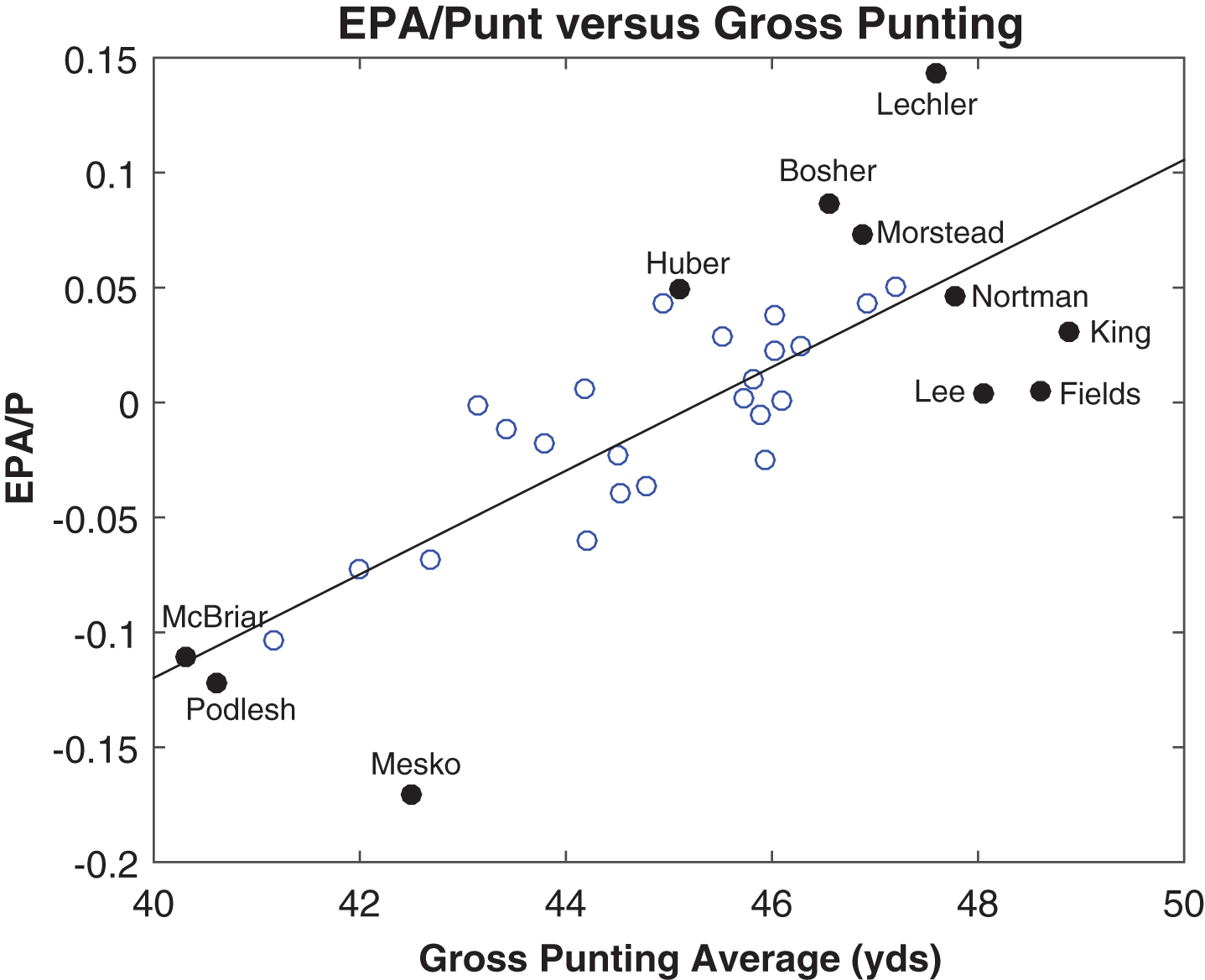
Fig.15
EPA per punt versus gross punting average, 2013.
3.3Addressing data availability
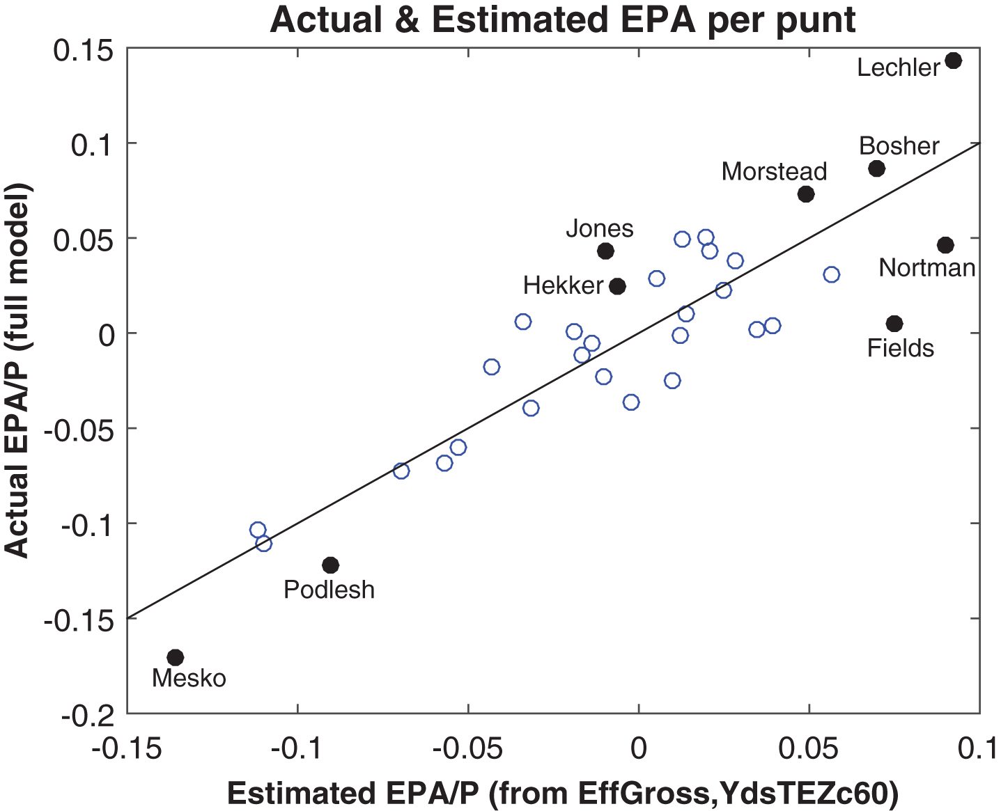
The multi-factor models developed in this paper are dependent on data that are not readily available, notably flight distance, hang time, and lateral landing point. As with other complex measures such as QBR or WAR, it can be useful to have methodology that allows for estimation based solely on more-accessible aggregate statistics. To this end, we note that in the 2013 season, EPA/P correlates well (+0.78) with gross punting average, as shown in Fig. 15. The correlation is higher (+0.82) for effective gross average, which adjusts for touchbacks. To get a meaningful alternative metric, a field-position measure is also needed, but merely taking the average pre-punt distance to the end zone (i.e. 100 – line of scrimmage, for punts taken from the punting team’s own territory) is inadequate. Typical gross punting distance is about the same across all long-field situations, as discussed in section 2.1. For this reason, we construct a field position measure by capping YdsTEZ at 60, then taking the average for each punter; as expected, this variable (YdsTEZc60) correlates negatively with EPA/P. Fitting to these two variables, we get the EPA estimate shown in Equation (2). Figure 16 compares the estimated and actual EPA/P values for each punter with 32+ punts (i.e. averaging two per game).
Fig.16
Actual EPA per punt versus an estimate using effective gross and field position, 2013.
(2)
4Applying the multi-factor EPA metric
4.12013 punting leaders
In applying our full model from section 3.2 to evaluate punter performance during the 2013 season, the full results are shown in Appendix A. The top punter, by a wide margin, was Shane Lechler of the Houston Texans, with +12.6 EPA and +0.143 EPA per punt (EPA/P). Among the 34 punters who averaged at least two punts per game, he ranked in the top five in gross (47.6 yds, 5th), effective gross (46.2 yds, 4th), fly (46.8 yds, 3rd), and hang time (4.60 sec, 2nd). It is notable that his team was 2– 14 and allowed 26.8 points per game defensively, perhaps contributing in the gap between his ranks in net (13th) and gross yardage. Lechler did not have the frequent long-field situations expected of a player on a weak team, but rather had the 9th shortest field position, reducing his opportunities to kick deep. He was also ranked #1 for the season by Pro Football Focus (PFF), whose proprietary ratings system (see Kluwe, 2014) involves play-by-play film evaluation. In EPA/P, Lechler was followed by Matthew Bowsher of the Atlanta Falcons (+5.86 EPA, +0.086 EPA/P) and Thomas Morstead of the New Orleans Saints (+4.48, +0.073), both of whom ranked in the league’s top ten in gross, net, effective gross, effective net, and hang time. Not surprisingly, each was also ranked in the PFF’s top five.
In contrast, consider two punters who were esteemed by traditional statistics but that we ranked significantly lower. Oakland Raiders rookie Marquette King and Miami Dolphins punter Brandon Fields were the top two in the league in both gross and net distance, and King was the leader in fly distance as well. However, both were near the bottom in touchback percentage and hang time, and benefitted from mild temperatures and routine long-field situations. As a result, they ranked 10th and 16th, respectively, in EPA/P, and neither was in PFF’s top ten. Despite his average performance by our metric, Fields was one of two punters named to the Pro Bowl, the league’s post-season “all-star” game, perhaps suggesting that those selections rely heavily on traditional average yardage statistics.
4.2Salaries and economic value
For our EPA/P metric to be a reasonable tool for analyzing a player’s value to his team, it must first measure a skill that is maintained over time. If punters’ EPA/P values fluctuate wildly over time, this would suggest that the metric is poorly designed and/or that punting outcomes are mostly random. If the latter were true, then it would be wasteful for a team to spend more to sign an “excellent” punter, as he would be unlikely to repeat his performance in subsequent seasons. If punting is mostly skill and EPA/P captures that skill, we would expect to see positive season-to-season correlations in EPA/P, because skill largely persists over time. That is, we would expect that players who have a high EPA/P in one season should tend to do so in the next season as well, and the same should be true of players who have a low EPA/P. For more on this topic, see Petti (2011) and Berri & Burke (2012).
With only a single season of EPA/P data, we are unable to make such an assessment, but we can compare the first half (weeks 1– 9) and second half (weeks 10– 17) of the 2013 season. When we do so, computing each punter’s EPA/P for each half of the season (dropping the three who did not have 16+ punts in each), then we obtain a first-half-to-second-half correlation of +0.67 in EPA/P. This is second only to hang time (+0.74) among our statistics, which is a good sign, although the sample sizes (number of punters and number of punts per half-season by each) are small. For comparison, the other correlations across half-seasons were fly +0.66, gross +0.57, net +0.46, effective gross +0.36, touchback percentage +0.19, and effective net +0.18.
In considering the economic value of a player at any condition, it is key to understand how his contribution compares to that of a replacement-level player, one who can be readily signed for near the league minimum salary. Because most teams carry only one punter on their roster and mid-season changes are uncommon, we lack sufficient data to set a baseline using the performance of backup players. The league’s worst punter in 2013, Zoltan Mesko of the Pittsburgh Steelers, had a -0.171 EPA/P over the first seven games before being released, but this is likely well below replacement level, which we will consider to be – 0.050 EPA/P, roughly the 20th percentile of starting punters. Over a typical season of 80 punts, this would lead to a value of -4 EPA for such a replacement level punter.
By this standard, league-leader Shane Lechler (+12.61 EPA) was 16.61 EPA better than a hypothetical replacement, while our second-best punter, Matthew Bosher, was 9.86 EPA better than a readily available substitute. If we assume that 35 EPA is equivalent to one win (Harvard, 2012), and that one marginal win in 2013 came at a price of $15 million in added salary (Stuart, 2013), then Lechler’s performance is worth almost half a win, and roughly $7 million in salary value, and Bosher’s value would be a bit over $4 million, provided that such performance is repeatable. These values are in addition to the salary for a replacement-level punter, which we estimate at $500,000, as the 2013 minimum salaries varied from $405,000 to $940,000, based on prior years of service (Nixon, 2013).
The highest-paid punter in 2013, Andy Lee of the San Francisco 49ers, had a salary (as measured by the amount counted toward the team salary cap) of just over $4 million, but ranked 17th by our metric, with +0.31 EPA. He was not alone, as the seven highest-paid punters, each with a salary of at least $2 million, had a negative EPA in aggregate; just two of the seven (Pat McAfee and Kevin Huber) had substantially above-average seasons.
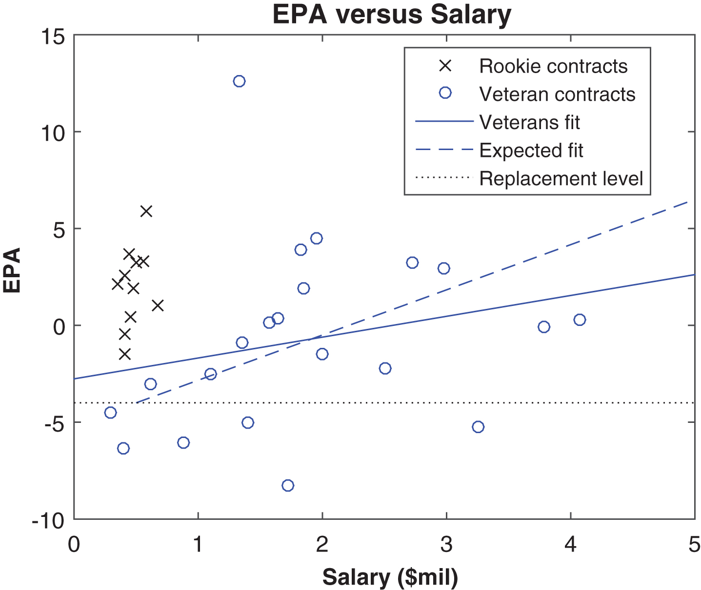
In analyzing the relationship between salary and performance, we first remove those players on rookie contracts, which have a salary and duration (3– 5 years) determined by the point at which the player was drafted. Among the 21 punters not on rookie contracts (whom we will call “veterans”) a linear regression showed that each additional million dollars of salary was associated with an increase of 1.08 EPA. This less than half of the slope that would be expected if one marginal win is associated with 35 additional EPA and $15 million of added salary; however, this slope depends on the replacement-level EPA that we establish. Figure 17 helps visualize the relationship between EPA and salary.
Veteran punters averaged – 0.75 EPA and a $1.86 million salary, while those on rookie contracts averaged +1.26 EPA and (neglecting two for whom we had no salary data) a $0.48 million salary. Punter is considered a position at which good players can have long careers (for example, Shane Lechler went on to play into his 40 s), and it seems unlikely that young players would consistently outperform higher-paid veterans, so the 2013 season may not be representative. Skills that do not figure into our rating system, such as avoiding blocked punts and fumbles, may be key in assessing value, although 2013 block rates were similar among the two groups. Teams who have to punt frequently, due to weak or conservative offenses, may also place higher value on a good punter, as the additional usage would likely increase the team’s return on investment.
Fig.17
EPA and salaries (“cap hit” value) in 2013, by contract status.
5Conclusion
Finding standard punter performance metrics to be inadequate, we have aggregated a data set fostering exploration of the effects of landing point, flight distance, and hang time on the field position value gained/lost subsequent to the football landing. Additionally, we have investigated the effects of environmental factors and coverage quality. A study of several consecutive seasons is needed would allow the opportunity to better quantify the impact (or lack thereof) of the various factors considered. Additionally, such a study would allow for computation of season-to-season correlations of evaluation metrics, an important step in establishing their credibility and evaluating the skill-versus-luck balance in punting statistics. A longer-term study would hold promise for bringing punter evaluation fully into the modern age of analytics, as was done for placekicker evaluation by Clark et al. (2013) and Pasteur & Cunningham-Rhoads (2014).
Acknowledgment
The authors wish to thank Brian Burke for his helpful suggestions that greatly improved the final paper.
Appendices
Appendix A
2013 Punter Metrics
| Punter (Team) | Salary* | EffGross | Fly | Hang | EPA | EPA/P |
| Shane Lechler (Texans) | 1.333 | 46.8 (3) | 46.2 (4) | 4.60 (2) | 12.61 (1) | 0.143 (1) |
| Matthew Bosher (Falcons) | 0.579 | 45.5 (11) | 46.0 (5) | 4.60 (4) | 5.86 (2) | 0.086 (2) |
| Thomas Morstead (Saints) | 1.950 | 46.2 (7) | 45.2 (9) | 4.51 (8) | 4.48 (3) | 0.073 (3) |
| Sam Martin (Lions) | 0.445 | 46.6 (4) | 44.4 (12) | 4.44 (14) | 3.65 (5) | 0.051 (4) |
| Kevin Huber (Bengals) | 2.720 | 44.6 (17) | 43.9 (16) | 4.44 (13) | 3.24 (8) | 0.049 (5) |
| Brad Nortman (Panthers) | 0.500 | 47.2 (2) | 46.3 (2) | 4.49 (11) | 3.26 (7) | 0.047 (6) |
| Steve Weatherford (Giants) | 1.825 | 46.0 (8) | 45.4 (7) | 4.22 (31) | 3.93 (4) | 0.043 (7) |
| Chris Jones (Cowboys) | 0.555 | 44.0 (20) | 43.4 (21) | 4.58 (6) | 3.29 (6) | 0.043 (8) |
| Pat McAfee (Colts) | 2.977 | 45.0 (13) | 44.7 (10) | 4.51 (9) | 2.92 (9) | 0.038 (9) |
| Marquette King (Raiders) | 0.405 | 47.4 (1) | 46.3 (3) | 4.30 (24) | 2.60 (10) | 0.031 (10) |
| Ryan Quigley (Jets) | 0.357 | 44.8 (15) | 44.7 (11) | 4.42 (15) | 2.10 (11) | 0.029 (11) |
| Johnny Hekker (Rams) | 0.483 | 45.7 (9) | 45.2 (8) | 4.65 (1) | 1.93 (13) | 0.025 (12) |
| Dustin Colquitt (Chiefs) | 1.850 | 44.9 (14) | 43.5 (19) | 4.35 (19) | 1.93 (12) | 0.022 (13) |
| Bryan Anger (Jaguars) | 0.676 | 44.2 (19) | 44.1 (14) | 4.52 (7) | 0.99 (14) | 0.010 (14) |
| Jeff Locke (Vikings) | 0.451 | 43.2 (23) | 43.4 (20) | 4.34 (20) | 0.41 (15) | 0.005 (15) |
| Brandon Fields (Dolphins) | 1.645 | 46.3 (6) | 47.0 (1) | 4.14 (32) | 0.39 (16) | 0.005 (16) |
| Andy Lee (49ers) | 4.075 | 46.3 (5) | 45.8 (6) | 4.47 (12) | 0.31 (17) | 0.004 (17) |
| Dave Zastudil (Cardinals) | 1.575 | 44.8 (15) | 44.2 (13) | 4.30 (23) | 0.16 (18) | 0.002 (18) |
| Shawn Powell (Bills) | 45.5 (10) | 43.2 (22) | 4.25 (29) | 0.02 (19) | 0.000 (19) | |
| Mike Scifres (Chargers) | 3.785 | 41.9 (28) | 42.8 (25) | 4.60 (5) | – 0.05 (20) | – 0.001 (20) |
| Ryan Allen (Patriots) | 0.406 | 44.5 (18) | 42.7 (26) | 4.32 (22) | – 0.44 (21) | – 0.006 (21) |
| Brett Kern (Titans) | 1.353 | 42.8 (25) | 42.6 (27) | 4.40 (18) | – 0.89 (22) | – 0.011 (22) |
| Spencer Lanning (Browns) | 0.405 | 42.5 (26) | 42.6 (28) | 4.27 (27) | – 1.48 (23) | – 0.018 (23) |
| Britton Colquitt (Broncos) | 2.000 | 43.5 (21) | 43.6 (17) | 4.60 (3) | – 1.49 (24) | – 0.023 (24) |
| Sam Koch (Ravens) | 2.500 | 45.0 (12) | 43.9 (15) | 4.29 (25) | – 2.22 (25) | – 0.025 (25) |
| Donnie Jones (Eagles) | 0.620 | 43.1 (24) | 43.6 (18) | 4.33 (21) | – 3.01 (27) | – 0.037 (26) |
| Tim Masthay (Packers) | 1.105 | 42.3 (27) | 43.0 (23) | 4.28 (26) | – 2.54 (26) | – 0.040 (27) |
| Michael Koenen (Buccaneers) | 3.250 | 43.4 (22) | 42.8 (24) | 4.40 (17) | – 5.26 (30) | – 0.060 (28) |
| Jon Ryan (Seahawks) | 1.405 | 41.7 (29) | 41.3 (30) | 4.50 (10) | – 5.05 (29) | – 0.068 (29) |
| Saverio Rocca (Redskins) | 0.878 | 40.4 (32) | 42.0 (29) | 4.22 (30) | – 6.06 (32) | – 0.072 (30) |
| Brian Moorman (Bills) | 0.392 | 40.6 (31) | 39.9 (33) | 4.41 (16) | – 6.32 (33) | – 0.104 (31) |
| Mat McBriar (Steelers) | 0.294 | 39.3 (33) | 38.9 (34) | 4.07 (34) | – 4.54 (28) | – 0.111 (32) |
| Adam Podlesh (Bears) | 1.725 | 38.8 (34) | 40.0 (32) | 4.08 (33) | – 8.29 (34) | – 0.122 (33) |
| Zoltan Mesko (Steelers) | 41.4 (30) | 41.3 (31) | 4.26 (28) | – 5.81 (31) | – 0.171 (34) |
Numbers in parentheses are rank among 34 players with 32+ punts on the season. *Salaries are in millions of US dollars, based on the amount counted toward the league salary cap.
References
1 | Berry D.A. & Berry T.D. , ((1985) ), The probability of a field goal: Rating kickers, The American Statistician 39: (2), 152–155. doi: 10.1080/00031305.1985.10479418 |
2 | Beuoy M. , ((2012) ), Are punters getting better? Available at: http://community.advancednflstats.com/2012/11/are-punters-getting-better.html (Accessed: 24 August 2016). |
3 | Bilder C.R. & Loughin T.M. , ((1998) ), “It’s good!” an analysis of the probability of success for Placekicks, CHANCE 11: (2), 20–30. doi: 10.1080/09332480.1998.10542087 |
4 | Burke B. , ((2008) ), Expected points. Available at: http://archive.advancedfootballanalytics.com/2008/08/expected-points.html (Accessed: 24 August 2016). |
5 | Burke B. , ((2010) ), Shane Lechler is overrated...or is he? Available at: http://archive.advancedfootballanalytics.com/2010/01/shane-lechler-is-overratedor-is-he.html (Accessed: 24 August 2016). |
6 | Burke B. , ((2014) a), Expected points and EPA explained. Retrieved August 24, 2016, from Advanced FootballAnalytics, http://www.advancedfootballanalytics.com/index.php/home/stats/stats-explained/expected-points-and-epa-explained |
7 | Burke B. , ((2014) b), Win probability and WPA explained Retrieved August 24, 2016, from Advanced FootballAnalytics, http://www.advancedfootballanalytics.com/index.php/home/stats/stats-explained/win-probability-and-wpa |
8 | Clark T.K., Johnson A.W. , & Stimpson A.J. , ((2013) ), Going for Three: Predicting the Likelihood of Field Goal Success with Logistic Regression, 2013 MIT Sloan Sports Analytics Conference. Available at: http://www.sloansportsconference.com/wp-content/uploads/2013/Going%for%Three%Predicting%the%Likelihood%of%Field%Goal%Success%with%Logistic%Regression.pdf (Accessed: 24 August 2016). |
9 | D’Errico J. , ((2005) ) Surface Fitting Using gridfit. Available at: https://www.mathworks.com/matlabcentral/fileexchange/-surface-fitting-using-gridfit (Accessed: 24 August 2016). |
10 | Gerrard B. , ((2007) ), Is the Moneyball approach transferable to complex invasion sports? International Journal of Sport Finance, 2: (4), 214–230. |
11 | Harvard Sports Analytics Collective, 2012, Calculating wins added in football: A First attempt. Availableat: http://harvardsportsanalysis.org/2012/01/calculating-wins-added-in-football-a-first-attempt/ (Accessed: 24 August 2016). |
12 | Kluwe C. , ((2014) ), Punt game: Sportsballing really hard with your foot. Available at: https://www.profootballfocus.com/punt-game-sportsballing-really-hard-with-your-foot/ (Accessed: 24 August 2016). |
13 | Lisk J. , ((2008) ), Pro Bowl Punters. http://www.pro-football-reference.com/blog/?p=563 Available at: (Accessed: 24 August 2016). |
14 | Morrison D.G. & Kalwani M.U. , ((1993) ), The best NFL field goal kickers: Are they lucky or good? CHANCE 6: (3), 30–37. doi: 10.1080/09332480.1993.10542375 |
15 | National Football League, 2016, NFL Quarterback Rating Formula. Retrieved August 24, 2016, http://www.nfl.com/help/quarterbackratingformula |
16 | Nixon J. , ((2013) ), NFL player salaries and benefits under the CBA. Available at: https://jeffnixonreport.wordpress.com/2013/04/23/nfl-player-salaries-and-benefits-under-the-cba/ (Accessed: 24 August 2016). |
17 | Oliver D. , ((2011) ), Guide to the total quarterback rating. Retrieved August 24, 2016, from ESPN, http://www.espn.com/nfl/story/_/id/6833215/explaining-statistics-total-quarterback-rating |
18 | Over the Cap, 2013, 2013 Punter Salaries. Retrieved August 7, 2017, https://overthecacom/position/punter/2013/ |
19 | Pasteur R.D. & Cunningham-Rhoads K. , ((2014) ), An expectation-based metric for NFL field goal kickers, Journal of Quantitative Analysis in Sports, 10: (1), 49–66. doi: 10.1515/jqas-2013-0039 |
20 | Picard R.R. & Cook D.R. , ((1984) ), Cross-validation of regression models, Journal of the American Statistical Association, 79: (387), 575–583. doi: 10.2307/2288403 |
21 | Romer D. , ((2006) ) Do firms maximize? Evidence from professional football, Journal of Political Economy, 114: (2), 340–365. doi: 10.1086/501171 |
22 | Stuart C. , ((2013) ), How to determine the appropriate salary cap values for veterans: Part I. Available at: http://www.footballperspective.com/how-to-determine-the-appropriate-salary-cap-values-for-veterans-part-i/ (Accessed: 24 August 2016). |
23 | Tymins A. , ((2014) ), Assessing the value of NFL punters. Available at: http://harvardsportsanalysis.org/2014/10/assessing-the-value-of-nfl-punters/ (Accessed: 24 August 2016). |


