Pitch actions that distinguish high scoring teams: Findings from five European football leagues in 2015-16

Sarkar, Sumit; Chakraborty, Soumyakanti

doi:10.3233/JSA-16161

Pitch actions that distinguish high scoring teams: Findings from five European football leagues in 2015-16

Article type: Research Article

Authors: Sarkar, Sumit^{; *} | Chakraborty, Soumyakanti

Affiliations: XLRI Jamshedpur, India

Correspondence: [*] Corresponding author: Sumit Sarkar, XLRI – Xavier School of Management, Jamshedpur 831001, India, Tel.: +91 657 6653172; Fax: +91 657 2227814; E-mail: [email protected].

Keywords: Team performance, determinants of goal, tactical variable, technical variable, log-linear regression, estimation

DOI: 10.3233/JSA-16161

Journal: Journal of Sports Analytics, vol. 4, no. 1, pp. 1-14, 2018

Published: 27 February 2018

Get PDF

Abstract

In order to find the determinants of non-penalty goals scored per match, in association football (soccer), this paper developed a regression model consisting of 8 explanatory variables, based on observations for 98 teams playing in the top tiers of club football in England, Spain, Germany, France and Italy. We started with a framework that considered twenty-one different pitch actions that included both technical and tactical variables. Using data for the 2015-16 football season we narrowed down to the 8 variable model. The paper used a log-linear regression model in order to remove heteroscedasticity. The model estimated the number of non-penalty goals per game with error of less than |0.33| for 93 teams out of 98. For 52 teams the margin of error was less than |0.1|. Shots from penalty box per game, share of shots from goal box in total shots and long pass accuracy were found to have statistically significant positive impact on non-penalty goals scored per game. Share of long passes in total passes and crosses per game have significant negative impact.

1Introduction

Over the last ten years performance analysis in association football¹ (soccer) has made some serious progress. A sizeable section of this body of research attempts to identify factors that influence team performances. Researchers have attempted to identify performance indicators that differentiate between successful and unsuccessful teams, both in tournament format competitions as well as in league competitions. Hughes and Bartlett (2002) defined performance indicators as a set of action variables that attempts to define at least some aspects of a performance. In case of tournaments, success has been generally defined by the stage of the competition reached by the team. For leagues, points scored and standing in the league table defined success. Success may depend on possession (Collet, 2013, James et al., 2004) high-intensity running and sprints undertaken (Di Salvo et al., 2009), passing (Saito et al., 2013, Scoulding et al., 2004), chance (Lagos, 2007), or even analysis of game related statistics (Lago-Penas et al., 2010). While success in a final game might depend on a few factors like shots on goal and effective goalkeeping (Szwarc, 2007), success in a league depends on multiple factors like goals to shots ratio, percentage of goals scored from outside the box, ratio of short to long passes, number of crosses, number of goals conceded and even number of yellow cards (Oberstone, 2009). There are studies that attempt to identify the determinants of the performance indicators. For example, Lago and Martin (2007) investigated the determinants of possession.

The most important determinant of success in football is scoring more goals than the number of goals conceded. While success depends on both offensive and defensive prowess of the team, a very low scoring team cannot win a season-long league. This in effect makes goal-scoring the most important activity on the pitch, in football leagues. Also, spectators spend their money and effort primarily to see goals. Scoring goals or creating goal-scoring opportunities depends on various technical and tactical parameters, as well as on the situation of the game. Research papers like Ensum et al. (2005), Hughes and Franks (2005), Konstadinidou and Tsigilis (2005), Janković et al. (2011)), Lago-Penas et al. (2010a) Tenga and Sigmundstad (2011), Wright et al. (2011) etc. identified various determinants including passing accuracy, shooting accuracy and success, possession, types of passes and passing sequences, attacking third entry, position of attempt and type of shoot, distance covered, formation etc. Another strand of literature focusses on identifying goal scoring patterns (Garganta et al., 1997, Yiannakos & Armatas, 2006, Armatas et al., 2007, Redwood-Brown, 2008, Armatas et al., 2009, Lago-Penas et al., 2010b, Tenga et al., 2010, Ridgewell, 2011, Mitrotasios & Armatas, 2014, Pratas et al., 2012) depending on time of goal scored, sequence of actions prior to goal, passing pattern before goal scoring, area of scoring attempt, type of attack and other situational variables.

2Method of analysis

Most of the studies mentioned in the previous section were done with data taken from international knock-out tournaments. One reason for choosing international knock-out tournaments like FIFA World Cup or UEFA European Championship is presence of larger number of teams vis-á-vis domestic leagues. A larger number of teams, and hence a larger number of observations, allows the researchers to consider a larger number of factors or explanatory variables that might have effect on goal scoring. It is not possible to study domestic leagues, where only 20 teams participate, considering a large number of explanatory variables. There will be very few degrees of freedom if the number of explanatory variables is increased with only 20 observations. In order to consider a large number of explanatory variables, in this paper we used 98 observations from English Premier League, La Liga, Bundesliga, Ligue One and Serie-A for the 2015-16 season. In order to find the determinants of average number of non-penalty². goals scored per game, we considered 8 technical or skill related variables, 11 tactical variables and 2 set-piece related variables as plausible determinants of non-penalty goals scored per game.

2.1Data source

We used data from whoscored.com, which is now an influential website for football (soccer) statistics. The data sources for whoscored.com³ are Opta Sports and eNetPlus, which are reliable and acceptable sources. The website provides rating for players as well as for teams and keeps the data available in public domain.

2.2Variables

Goal scoring ability of a football team may depend on five different kinds of pitch actions – (1) shots, (2) passes, (3) crosses, (4) set-pieces, (5) dribbles, (6) aerial balls and (7) possession. Some of these pitch actions can be broken into finer details. We considered pitch actions as illustrated in Fig. 1.

Fig.1

Pitch actions that create goal scoring opportunities.

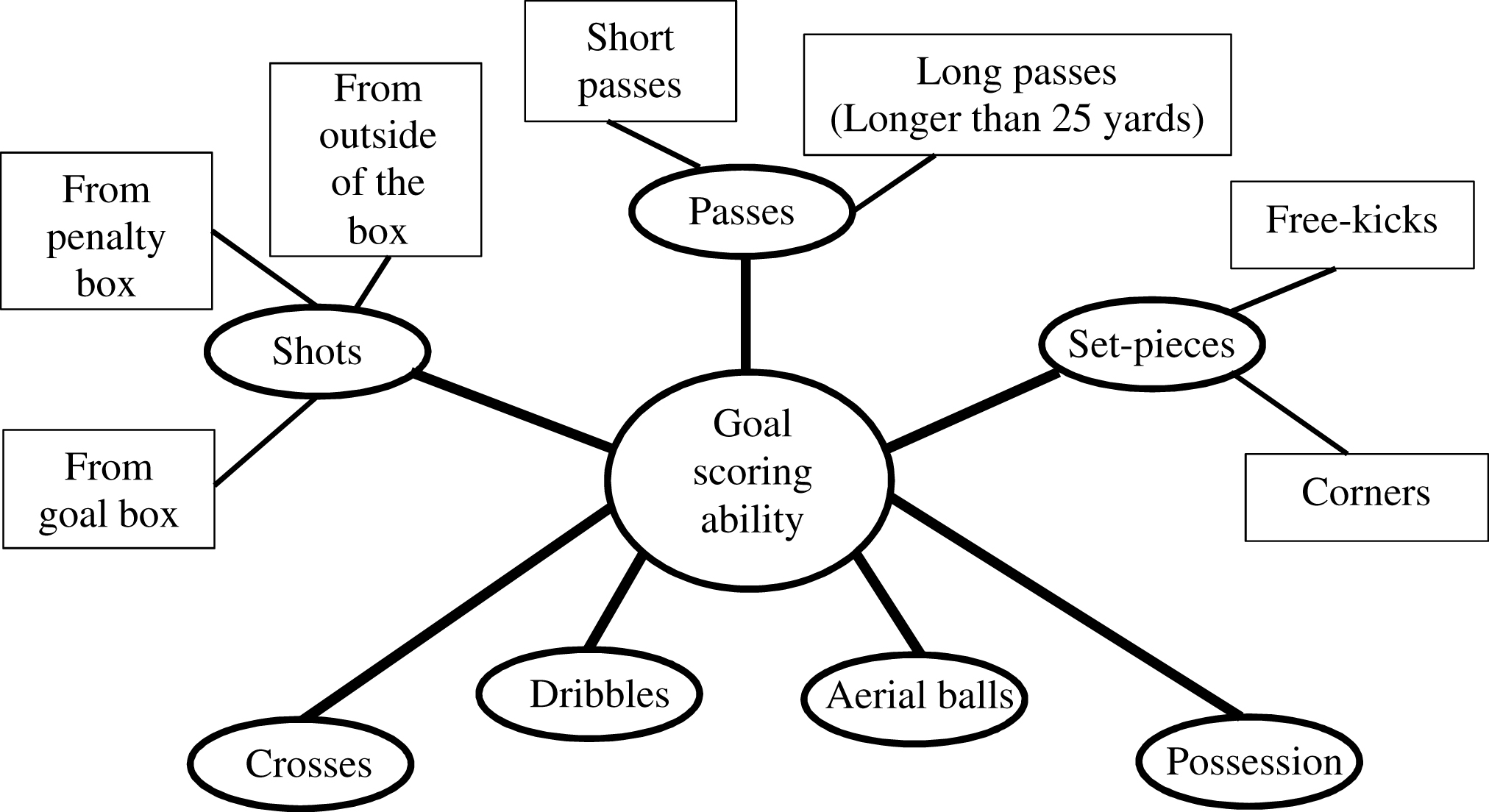
Goal box is the six yard box. Penalty box is the 18 yard box. “Shots” means shots taken at goal with intent of scoring. “Shots from penalty box” means the shots taken from inside the 18 yard box but outside the six yard box. Penalty kicks are also taken from the spot inside the 18 yard box, but outside the six yard box. However, penalty kicks are not included in “shots from penalty box”. The pitch actions are explained in Table 1.

Table 1

Explanation of pitch actions

Pitch-action	Explanation
“Shots from penalty box”	Shots taken at goal with intent of scoring from inside the 18 yard box but outside the six yard box, excluding penalty kicks.
“Shots from goal box”	Shots taken at goal with intent of scoring from inside the six yard box.
“Passes”	Passing the ball to a team-mate.
“Crosses”	Passes from a wide position to a central attacking area.
“Dribbles”.	Taking on an opponent and successfully making it past them whilst retaining the ball
“Set-pieces”	Pitch actions that resume the game from a dead-ball situation.
“Free-kick”	The kick that resumes the game after a foul. The team that was fouled against gets the free-kick.
“Corner”	The kick from the corner that resumes the game if the ball crosses the goal line (outside the goal posts) with a touch from the defending team. The attacking team gets the corner kick.
“Aerial ball”	A situation when the ball is air borne.
“Possession”	A team retains “possession” if the ball is under the control of the team, excluding dead-ball situations. “Possession” data is available as a percentage of time during which a team retains possession, out of total time that the ball is in active play during the game.

Out of these pitch actions we created 21 variables, which can be classified into three categories – (A) technical or skill related, (B) tactical and (C) set-pieces earned, as summarized in Table 2. The technical variables are measures of accuracy and of success of different pitch actions, and depend on the skill level of the players and coordination among team-mates. However, whether to play long passes or short passes, whether to attempt a shot on goal from outside the box or from within the box, whether to attempt dribbles or rely on passing, whether to play from the wide positions and to attempt crosses, and whether to have possession or to let the opponent have possession are tactical decisions made by the manager and the coaching staff. We have classified such variables as tactical variables. Earning free-kicks and corners depends on the how much a team can press on the opponent as well as on the referee. That’s why we kept those variables in aseparate category. We have calculated the values of each of these explanatory variables for each of the 98 teams in the five leagues using the data collected from whoscored.com. The data was collected on 18th May of 2016, after all the games in all the five leagues werecompleted.

Table 2

Definitions of explanatory variables

Technical (skill related) variables	Tactical variables	Set-pieces earned
1. Shooting accuracy (SHACC) =(Totalshots-Shotswide)Totalshots×100	1. Shots from out of box per game (SHOB) =TotalshotsfromoutofboxNumberofgames	1. Corners per game (COPG) =TotalcornersearnedNumberofgames
2. Short pass accuracy (SPACC) =AccurateshortpassesTotalshortpasses×100	2. Shots from penalty box per game (SHPB) =TotalshotsfrompenaltyboxNumberofgames	2. Free-kicks per game (FKPG) =TotalfreekicksearnedNumberofgames
3. Long pass accuracy (LPACC) =AccuratelongpassesTotallongpasses×100	3. Shots from goal box per game (SHGB) =TotalshotsfromgoalboxNumberofgames
4. Cross accuracy (CRACC) =AccuratecrossesTotalcrosses×100	4. Share of shots from penalty box (SHSPB) =shotsfrompenaltyboxTotalshots×100
5. Corner accuracy (COACC) =AccuratecornersTotalcorners×100	5. Share of shots from goal box (SHSGB) =shotsfromgoalboxTotalshots×100
6. Free-kick accuracy (FKACC) =Accuratefree-kicksTotalfree-kicks×100	6. Short passes per game (SPPG) =TotalshotspassesNumberofgames
7. Dribbling success (DRSUC) =SuccessfuldribblesDribblesattempted×100	7. Long passes per game (LPPG) =TotallongpassesNumberofgames
8. Aerial success (ARSUC) =AerialswonTotalaerialballs×100	8. Share of long passes (SHLP) =TotallongpassesTotalpasses×100
	9. Crosses per game (CRPG) =TotalcrossesNumberofgames
	10. Dribbles attempted per game (DRPG) =TotaldribblesattemptedNumberofgames
	11. Possession (POSSH) =PossessiontimeTimetheballisinactiveplay×100

All passes were classified as either short passes (less than 25 yards long) or long passes (more than 25 yards long). Therefore, percentage share of short passes is only (100 – percentage share of long passes). Hence, instead of considering percentage share of long passes as well as that of short passes, we considered only the percentage share of long passes. Similarly, all shots were classified as either from outside of the box, or from inside the penalty box (but outside the goal box), or from inside the goal box. Since we considered percentage share of shots from penalty box as well as that from goal box, there is no reason to take the percentage share of shots from out of box separately.

2.3Building the multiple regression model

Since we are interested in finding the determinants of non-penalty goals scored per game (NPGPG) ⁴, it becomes our dependent variable. NPGPG is defined as

NPGPG=Totalnon-penaltygoalsscoredbyateamNumberofgamesplayedbytheteam

Among the five leagues from which we took data, all except Bundesliga had 20 teams and hence each team played 38 matches during the season. But Bundesliga had 18 teams and hence the Bundesliga teams played 34 matches each during the season. Because of this asymmetry in number of games played by teams, we took non-penalty goals scored per game as our dependent variable, instead of total non-penalty goals.

We understand that some of the 21 explanatory variables defined in Table 2 may be highly correlated resulting in presence of multicollinearity⁵. After checking pairwise correlation, we removed at least one of the variables among those that had pairwise correlation coefficients higher than |0.8|. In order to retain the maximum number of variables we used a simple rule. If a variable is pairwise correlated with more than one variable, but the variables with which it is correlated are correlated only with this variable, then we removed this variable only. Five variables that we eliminated are SHGB, SPACC, SPPG, FKACC and POSSH. The correlation matrix is given in the Appendix (Table A1).

Using Eviews 6, we ran the following linear regression model.

(1)

NPGPGi=α+β1SHACCi+β2SHOBi+β3SHPBi+β4SHSGBi+β5SHSPBi+β6LPACCi+β7LPPGi+β8SHLPi+β9CRACCi+β10COACCi+β11CRPGi+β12COPGi+β13FKPGi+β14DRSUCi+β15DRPGi+β16ARSUCi+ui

where i is the name of the team, i = [1, 98], βk is the coefficient of the kth variable, α is the constant term and u_i is the residual term for the ith observation.

The regression result is given in Table A2 (see appendix). Though the adjusted R² is high (0.7998) and the probability value of the F-statistic is 0, indicating that the model is overall statistically significant, we can see from Table A2 (in the Appendix) that the t-statistic is significant (higher than 1.98)⁶ for only 5 variables. This might be due to further presence of multicollinearity, or due to presence of heteroscedasticity⁷, or because the residuals are not normally distributed. Looking at the scatter diagrams for NPGPG against some of the explanatory variables we suspected presence of heteroscedasticity. Since our sample is sufficiently large, we ran a White test for the model (1). The result of the test is given in Table 3. Since the probability values for both F-statistic as well as that of the χ² are less than 0.05, we couldn’t rule out presence of heteroscedasticity at 5% level.

In presence of heteroscedasticity the estimators fail to be BLUE (Best Linear Unbiased Estimator), and the model (1) is not acceptable. As an additional diagnostic test we ran the Jarque-Bera test on model (1) to see if the residuals are nearly normally distributed. The result is shown in Fig. 2. The Jarque-Bera (JB)⁸ statistic is high and the probability is low, we reject the hypothesis that the residuals are normally distributed.

Fig.2

Histogram of residuals for model (1).

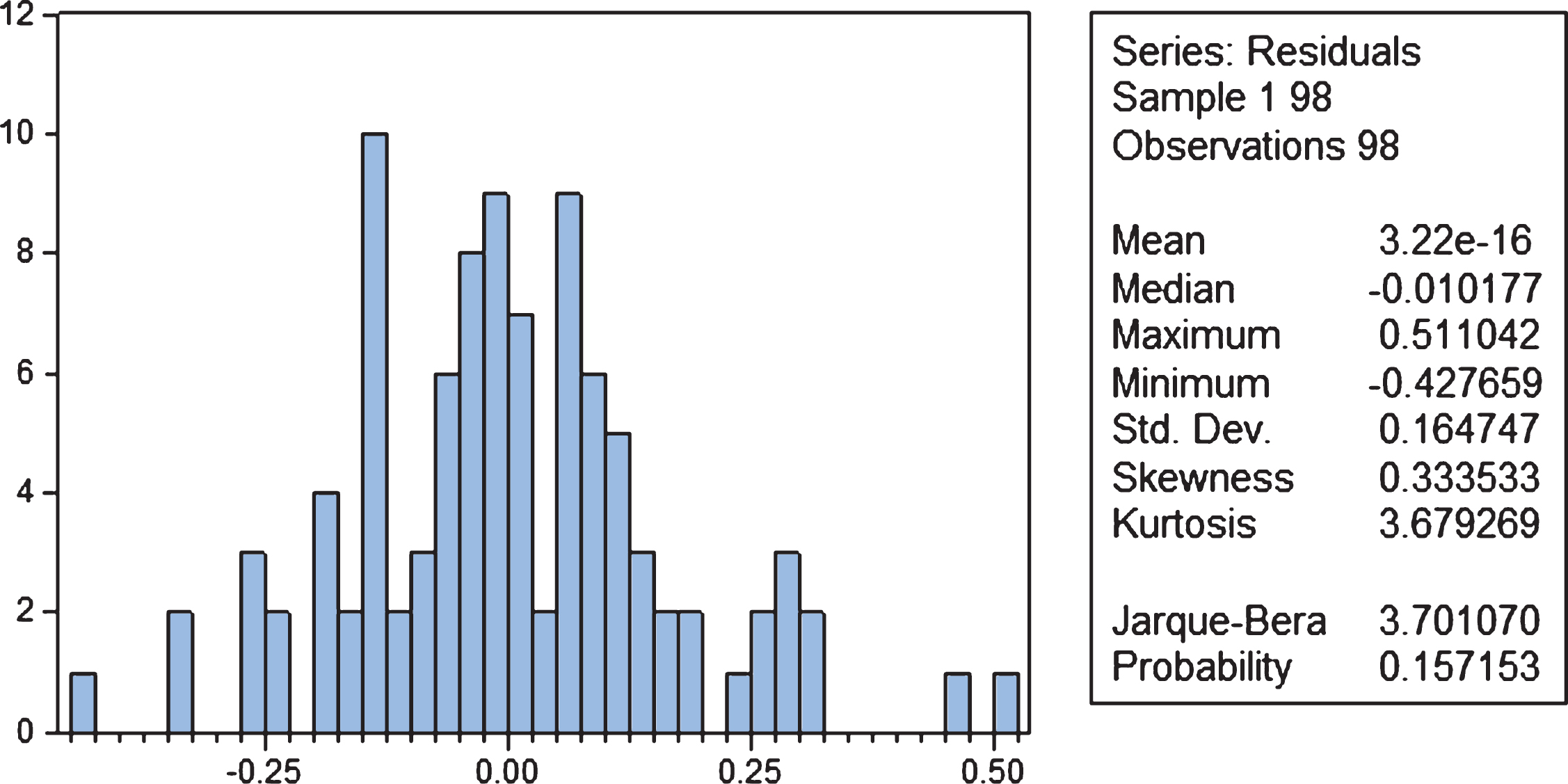
Table 3

White Heteroscedasticity Test for Model (1)

F-statistic	2.783193	Prob. F(16,81)	0.0013
Obs*R-squared	34.76467	Prob. Chi-Square(16)	0.0043

Since there exists heteroscedasticity and the residuals are not normally distributed, we need to change the model (1). A log transformation is likely to reduce heteroscedasticity because it compresses the scales in which the variables are measured. Taking a log transformation of the model (1) we constructed the following model and ran the regression.

(2)

ln(NPGPGi)=α′+β1′.ln(SHACCi)+β2′.ln(SHOBi)+β3′.ln(SHPBi)+β4′.ln(SHSGBi)+β5′.ln(SHSPBi)+β6′.ln(LPACCi)+β7′.ln(LPPGi)+β8′.ln(SHLPi)+β9′.ln(CRACCi)+β10′.ln(COACCi)+β11′.ln(CRPGi)+β12′.ln(COPGi)+β13′.ln(FKPGi)+β14′.ln(DRSUCi)+β15′.ln(DRPGi)+β16′.ln(ARSUCi)+ui

where i is the name of the team, i = [1, 98], β^*_k is the coefficient of the kth variable, α^* is the constant term and u_i is the residual term for the ith observation.

The result of regression run on model (2) is given in Table A3 in the Appendix. The high adjusted R² (0.7598) and 0 probability value of the F-statistic indicates that the model is overall statistically significant. Though the adjusted R² is slightly less than that of model (1), we chose model (2) over model (1) on basis of AIC (Akaike Information Criteria)⁹ and SIC (Schwarz Information Criteria)¹⁰ .

The purpose of developing model (2), rejecting model (1), was the presence of heteroscedasticity in model (1). As a diagnostic test we ran the White test on model (2). The result of the test is given in Table 4.

Table 4

White Heteroscedasticity Test for Model (2)

F	statistic	1.387674	Prob. F(16,81)	0.1689
Obs*R	squared	21.08347	Prob. Chi Square(16)	0.1753

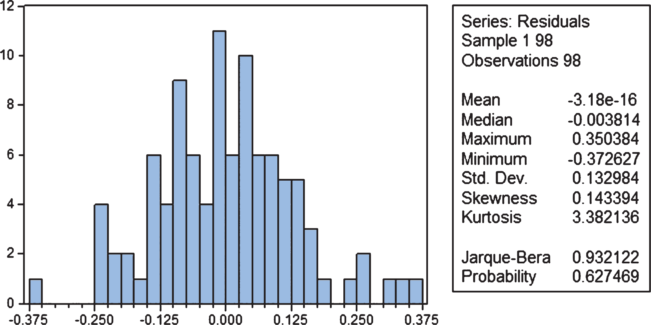
Since the probability values for both F-statistic as well as that of the χ² are more than 0.05, we can rule out presence of heteroscedasticity at 5% level. We also ran the Jarque-Bera test on model (2) to see if the residuals are nearly normally distributed. The result is shown in Fig. 3. Since the JB statistic is low (less than 1) and the probability is high (0.6275), we conclude that the residuals are normally distributed. The Durbin-Watson d-statistic is 1.8825, suggesting that there is no autocorrelation¹¹. This means, model (2) satisfies all conditions for the estimators to be BLUE. Despite that, the t-statistic are not significant for most of the variables (Refer to Table A3 in the Appendix). That must be due to presence further of multicollinearity. In such a scenario the practice is to first remove the explanatory variables with t-statistic < |1|. From Table A3 (given in the Appendix) it can be seen that the t-statistic is in the interval (–1, 1) for ln(SHACC), ln(SHOB), ln(SHSPB), ln(LPPG), ln(DRSUC), ln(DRPG) and ln(ARSUC). Removing these seven explanatory variables we reconstructed the regression model as:

(3)

ln(NPGPGi)=α″+ β″1.ln(SHPBi)+ β″2.ln(SHSGBi)+ β″3.ln(LPACCi)+ β″4.ln(SHLPi)+ β″5.ln(CRACCi)+β″6.ln(COACCi)+ β″7.ln(CRPGi)+ β″8.ln(COPGi)+ β″9.ln(FKPGi)+ui

where i is the name of the team, i = [1, 98], β^*_k is the coefficient of the kth variable, α^* is the constant term and u_i is the residual term for the ith observation.

Fig.3

Histogram of residuals for model (2).

The result of the regression run on model (3) is given in Table A4 (see Appendix). The adjusted-R² (0.7662) is higher than that of model (2). More importantly, the AIC (–0.9475) and SIC (–0.6837) values are less than those for model (2). This indicates that the variables removed were irrelevant and hence model (3) is a better model than model (2). To be sure we ran the White test (to check heteroscedasticity) and the Jarque-Bera test (to check normality of the residuals) on model (3). The results of both tests were negative, i.e., we could reject heteroscedasticity and accept the hypothesis that the residuals are normally distributed. The Durbin-Watson d-statistic is 1.9986, which indicates that there is no autocorrelation either. The t-statistic is significant¹² for ln(SHPB), ln(SHSGB), ln(LPACC), ln(SHLP) and ln(CRPG). For the other variables, except ln(COPG), the t-statistic are larger than |1|.

Since the t-statistic for ln(COPG) is –0.6166, we removed the variable in our next level of iteration and reconstructed the regression model asfollows:

(4)

ln(NPGPGi)=α*+β1*.ln(SHPBi)+ β2*.ln(SHSGBi)+β3*.ln(LPACCi)+ β4*.ln(SHLPi)+β5*.ln(CRACCi)+ β6*.ln(COACCi)+β7*.ln(CRPGi)+ β8*.ln(FKPGi)+ui

where i is the name of the team, i = [1, 98], β^*_k is the coefficient of the kth variable, α^* is the constant term and u_i is the residual term for the ith observation.

The result of regression run on model (4), as given in Table A5 of the appendix, suggests that model (4) is the most suitable regression model for estimating the determinants of non-penalty goals per game. There is no explanatory variable with t-statistic in the interval (–1, 1). The adjusted-R² (0.7678), AIC (–0.9636) and SIC (–0.7261) are all better than those of model (3). To be sure we ran White test to rule out heteroscedasticity and Jerque-Bera test to ensure that the residuals are normally distributed. The tests affirmed homoscedasticity (i.e., rules out heteroscedasticity) and normality of residuals. The Durbin-Watson d-statistic is 2.0082, indicating that there is no autocorrelation.

3Estimation results

The estimated coefficients along with standard error, t-statistic and probability values for the explanatory variables of model (4) are given in Table 5.

Table 5

Estimated coefficients for model (4)

Variable	Coefficient	Std. Error	t-Statistic	Probability
Intercept	–1.671867	0.905649	–1.846044	0.0682
ln(SHPB)	0.882545	0.114766	7.689918	0
ln(SHSGB)	0.228343	0.050063	4.561079	0
ln(LPACC)	0.461721	0.176174	2.620819	0.0103
ln(SHLP)	–0.208549	0.093095	–2.240185	0.0276
ln(CRACC)	–0.283465	0.151239	–1.874283	0.0642
ln(COACC)	0.154993	0.100587	1.540875	0.1269
ln(CRPG)	–0.273781	0.078123	–3.504483	0.0007
ln(FKPG)	–0.124845	0.092989	–1.34258	0.1828

Since the degrees of freedom of the model is 89, the t-statistic are significant when greater than |1.98|. As can be seen from Table 4, the t-statistic are significant for ln(SHPB), ln(SHSGB), ln(LPACC), ln(SHLP) and ln(CRPG). Using the coefficients from Table 4 we can write our estimation equation as:

(4E)

ln(NPGPGi)=-1.671867+0.882545ln(SHPBi)+0.228343ln(SHSGBi)+0.461721ln(LPACCi)-0.208549ln(SHLPi)-0.283465ln(CRACCi)+0.154993ln(COACCi)-0.273781ln(CRPGi)-0.124845ln(FKPGi)4E

or,

(4E′)

NPGPGie-1.671867[SHPBi0.882545.SHSGBi0.228343.LPACCi0.461721.COACCi0.154993SHLPi0.208549.CRACCi0.283465.CRPGi0.273781.FKPGi0.124845]

where, i is the name of the team, i = [1, 98].

Using equation (4E’) and the real values of the explanatory variables we estimated the non-penalty goals scored per game for each of the 98 teams and compared against the actual values of the variables. The comparison of actual NPGPG and estimated NPGPG for the top 14 teams (in terms of actual NPGPG) is given in Table 6.

Table 6

Estimated NPGPG for 14 top scoring (per game) teams

Team	NPGPG	Estimated (NPGPG)
Real Madrid	2.684211	1.9472931
Barcelona	2.578947	2.570044
Paris Saint Germain	2.5	2.3528469
Borussia Dortmund	2.235294	2.2050714
Roma	2.078947	1.4751239
Bayern Munich	2.058824	2.3938306
Napoli	1.868421	1.9220011
Borussia M.Gladbach	1.794118	1.512193
Manchester City	1.736842	1.7279739
Juventus	1.684211	1.4954365
Tottenham	1.657895	1.5388236
Lyon	1.657895	1.6948561
Atletico Madrid	1.605263	1.3158287
Arsenal	1.605263	2.0587247

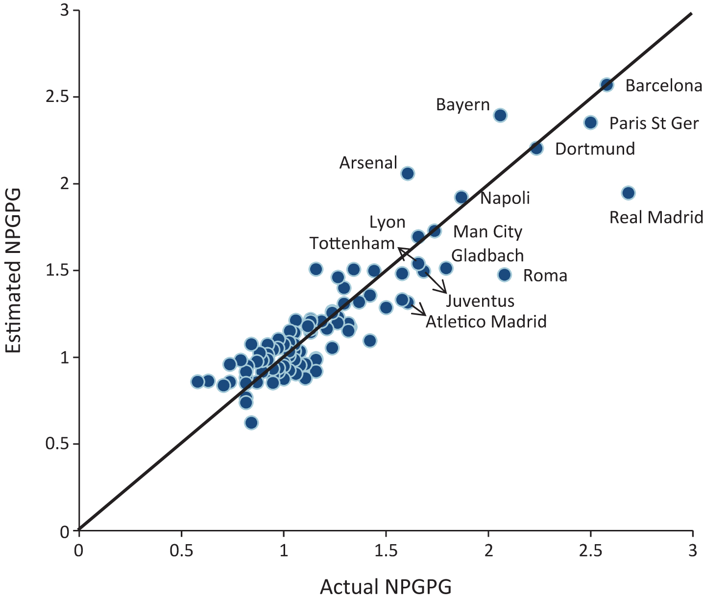
The scatter plot of estimated NPGPG against actual NPGPG for all the 98 teams is shown in Fig. 4. We have marked the scatter plots of the top 14 teams in the scatter diagram. Our estimates almost perfectly matched with actual values for Barcelona, Dortmund, Napoli, Manchester City and Lyon among the top 14 teams, and for many other teams.

Among the top 14, we underestimated Paris St. Germain, Juventus and Tottemham by a margin of less than 0.2. Atletico Madrid and Borussia M.Gladbach were underestimated by margins less than 0.3. Bayern and Arsenal were overestimated, while Real Madrid and Roma were underestimated by margins more than 0.33. Margin for Bayern was just –0.335. Among all 98 teams we underestimated only 2 teams (Real Madrid and Roma) and overestimated only 3 teams (Arsenal, Sevilla and Bayern) with a margin more than 0.33. For 93 teams ourmargin of error was less than |0.33| and for 52 teams our margin of error was less than |0.1|. Refer to Table A6 in the Appendix.

Fig.4

Scatter diagram of estimated NPGPG against actual NPGPG.

4Discussion and conclusion

In this paper we tried to identify the pitch actions (both technical and tactical) that significantly affect goal scoring. Regression models developed on observations from five leagues in Europe during the season 2015-16 shows that the number of shots from penalty box, per game, is the most important determinant of non-penalty goals per game. This result is supported by our log-linear regression model developed on basis of observations for all 98 teams as well as by the model developed on basis of the observations for the 35 teams that scored above average number of non-penalty goals per game. From the regression model (4) we conclude that increasing the share of shots from goal box increases the number of goals. That means it is a better strategy to attempt goals from close range than from a distance.

We believe that the coaches and managers may find the following result useful. Share of long passes in total passes and number of crosses played per game adversely affects goal scoring, but accuracy of long passes positively impact it. Technical perfection in long passes and passes in general is required, but strategically it is better to increase the number of shot passes played per long pass. This is what Johan Cruyff and his spiritual disciples in football strategy like Arsene Wenger or Pep Guardiola, have been saying for ages and we have seen great teams like Ajax (1971-74), Netherlands national team (1972-78), Barcelona (1992-94 and 2008 to present), Bayern Munich (2012 to present) and Arsenal (1997–2007) that successfully employed the strategy. In the season 2015-16 we have seen teams like Barcelona, Bayern, Dortmund, Manchester City, Arsenal, Paris Saint Germain etc. apply that strategy.

Number of crosses, per game, increases if a team tends to attack from the wide. While it is a might be a good strategy to employ full backs to go on occasional overlaps, playing from the wide reduces the goal scoring opportunity. When a team attacks from the wide, the centre backs of the opposition gets more time and can anticipate the crosses. This result is juxtaposed to Mara et al. (2012), which showed that in 2010-11 season of W-league¹³ 24% goals were scored from crosses. That might be a serious difference between women’s game and the men’s game.

Appendices

Appendix

Table A1

Correlation matrix* of explanatory variables (observations from all 98 teams)

	SHACC	SHOB	SHGB	SHPB	SHSGB	SHSPB	SPACC	LPACC	SPPG	LPPG	SHLP	CRACC	COACC	FKACC	CRPG	COPG	FKPG	DRSUC	DRPG	ARSUC	POSSH
SHACC	1
SHOB	0.16	1
SHGB	0.21	0	1
SHPB	0.5	0.32	0.55	1
SHSGB	0	–0.4	0.87	0.14	1
SHSPB	0.33	–0.6	0.31	0.57	0.27	1
SPACC	0.45	0.36	0.12	0.43	–0.2	0.06	1
LPACC	0.34	0.36	0.29	0.56	0	0.13	0.72	1
SPPG	0.51	0.38	0.33	0.65	0	0.21	0.83	0.76	1
LPPG	–0.3	–0.2	–0.4	–0.4	–0.2	–0.2	–0.6	–0.4	–0.6	1
SHLP	–0.5	–0.3	–0.3	–0.6	0.06	–0.2	–0.9	–0.7	–0.9	0.79	1
CRACC	0.01	–0.1	0.12	0.38	0.02	0.45	–0.1	0.14	0.02	0.1	0.03	1
COACC	0.28	0.24	0.14	0.42	–0.1	0.15	0.51	0.51	0.52	–0.2	–0.5	0.15	1
FKACC	0.44	0.38	0.16	0.48	–0.1	0.11	0.83	0.76	0.81	–0.6	–0.8	0.02	0.54	1
CRPG	–0.1	0.15	0.24	0.05	0.21	–0.1	0.16	0.13	–0.1	–0.1	–0	–0.2	0.06	0	1
COPG	0.47	0.44	0.53	0.67	0.21	0.17	0.47	0.45	0.5	–0.4	–0.5	–0	0.39	0.47	0.51	1
FKPG	–0.1	0.07	–0.1	–0.1	–0.1	–0.1	–0.1	–0	0.02	0	–0	0.1	0.02	0.19	–0.4	–0.2	1
DRSUC	0.15	0.28	0.15	0.17	0.02	–0.1	0.56	0.36	0.41	–0.4	–0.5	–0.1	0.29	0.38	0.22	0.24	–0.2	1
DRPG	0.45	0.14	0.24	0.47	0.01	0.27	0.47	0.39	0.51	–0.4	–0.5	0.15	0.34	0.41	–0.1	0.36	0	0.09	1
ARSUC	0.06	0.24	0.33	0.44	0.14	0.13	0.25	0.54	0.38	–0.3	–0.3	0.23	0.24	0.29	0.16	0.3	0	0.17	0.1	1
POSSH	0.52	0.42	0.35	0.66	0	0.19	0.83	0.76	0.96	–0.6	–0.9	0.02	0.56	0.8	0.02	0.57	0.04	0.38	0.52	0.38	1

*Correlation coefficients greater than |0.8| are shown in bold.

Table A2

Regression results for Model (1)

Dependent Variable: NPGPG
Method: Least Squares
Date: 05/26/16 Time: 10 : 45
Sample: 1 98
Included observations: 98
Variable	Coefficient	Std. Error	t-Statistic	Probability
Intercept	1.286114	1.413842	0.909659	0.3657
SHACC	–0.000966	0.007971	–0.121247	0.9038
SHOB	–0.034301	0.102735	–0.333882	0.7393
SHPB	0.285317	0.080596	3.540082	0.0007
SHSGB	0.044929	0.01868	2.405202	0.0184
SHSPB	–0.020309	0.02299	–0.883408	0.3796
LPACC	0.012102	0.005605	2.159029	0.0338
LPPG	0.001139	0.005431	0.209676	0.8344
SHLP	–0.020834	0.013663	–1.524873	0.1312
CRACC	–0.019634	0.009122	–2.152418	0.0343
COACC	0.005908	0.003207	1.842044	0.0691
CRPG	–0.014817	0.007463	–1.985356	0.0505
COPG	–0.082692	0.049987	–1.654268	0.1019
FKPG	–0.014526	0.009567	–1.518345	0.1328
DRSUC	–0.003186	0.00407	–0.782797	0.436
DRPG	–0.003249	0.007817	–0.415644	0.6788
ARSUC	0.001775	0.007373	0.240756	0.8104
R-squared	0.832827	Mean dependent var		1.191319
Adjusted R-squared	0.799805	S.D. dependent var		0.402935
S.E. of regression	0.180286	Akaike criterion (AIC)		–0.432128
Sum squared resid	2.632736	Schwarz criterion (SIC)		0.016285
Log likelihood	38.17428	Hannan-Quinn criter.		–0.250754
F-statistic	25.22054	Durbin-Watson stat		1.940754
Prob(F-statistic)	0
Heteroskedasticity Test: White
F-statistic	2.783193	Prob. F(16,81)		0.0013
Obs*R-squared	34.76467	Prob. Chi-Square(16)		0.0043
Scaled explained SS	31.81576	Prob. Chi-Square(16)		0.0106

Table A3

Regression results for Model (2)

Dependent Variable: LOG(NPGPG)
Method: Least Squares
Date: 05/26/16 Time: 10 : 50
Sample: 1 98
Included observations: 98
Variable	Coefficient	Std. Error	t-Statistic	Probability
Intercept	–2.857617	5.476562	–0.52179	0.6032
LOG(SHACC)	–0.038274	0.36859	–0.103839	0.9176
LOG(SHOB)	0.360672	0.572547	0.629943	0.5305
LOG(SHPB)	0.735303	0.582358	1.262631	0.2103
LOG(SHSGB)	0.32612	0.106491	3.062409	0.003
LOG(SHSPB)	0.381971	1.289613	0.29619	0.7678
LOG(LPACC)	0.361251	0.22081	1.636027	0.1057
LOG(LPPG)	0.212954	0.331558	0.642281	0.5225
LOG(SHLP)	–0.36281	0.186212	–1.948366	0.0548
LOG(CRACC)	–0.246438	0.167849	–1.468217	0.1459
LOG(COACC)	0.175058	0.109317	1.601379	0.1132
LOG(CRPG)	–0.222839	0.11214	–1.987152	0.0503
LOG(COPG)	–0.199822	0.194415	–1.02781	0.3071
LOG(FKPG)	–0.144164	0.101425	–1.421389	0.159
LOG(DRSUC)	–0.098346	0.176044	–0.558643	0.5779
LOG(DRPG)	–0.046558	0.103884	–0.448176	0.6552
LOG(ARSUC)	–0.045957	0.296661	–0.154913	0.8773
R-squared	0.799388	Mean dependent var		0.128164
Adjusted R-squared	0.75976	S.D. dependent var		0.296906
S.E. of regression	0.145526	Akaike criterion (AIC)		–0.860498
Sum squared resid	1.715413	Schwarz criterion (SIC)		–0.412085
Log likelihood	59.16438	Hannan-Quinn criter.		–0.679124
F-statistic	20.17272	Durbin-Watson stat		1.882553
Prob(F-statistic)	0
Heteroskedasticity Test: White
F-statistic	1.387674	Prob. F(16,81)		0.1689
Obs*R-squared	21.08347	Prob. Chi-Square(16)		0.1753
Scaled explained SS	17.15522	Prob. Chi-Square(16)		0.3756

Table A4

Regression results for Model (3)

Dependent Variable: LOG(NPGPG)
Method: Least Squares
Date: 05/26/16 Time: 12 : 15
Sample: 1 98
Included observations: 98
Variable	Coefficient	Std. Error	t-Statistic	Probability.
Intercept	–1.634355	0.910852	–1.794314	0.0762
LOG(SHPB)	0.939788	0.147923	6.353218	0
LOG(SHSGB)	0.231661	0.050526	4.58499	0
LOG(LPACC)	0.457764	0.176908	2.587592	0.0113
LOG(SHLP)	–0.215629	0.094123	–2.290922	0.0244
LOG(CRACC)	–0.311455	0.158411	–1.96612	0.0524
LOG(COACC)	0.16542	0.102346	1.616282	0.1096
LOG(CRPG)	–0.239408	0.096194	–2.488807	0.0147
LOG(COPG)	–0.105076	0.170402	–0.616638	0.5391
LOG(FKPG)	–0.123662	0.093334	–1.324943	0.1886
R-squared	0.787861	Mean dependent var		0.128164
Adjusted R-squared	0.766165	S.D. dependent var		0.296906
S.E. of regression	0.143573	Akaike criterion (AIC)		–0.94749
Sum squared resid	1.813972	Schwarz criterion (SIC)		–0.683718
Log likelihood	56.427	Hannan-Quinn criter.		–0.840799
F-statistic	36.31368	Durbin-Watson stat		1.998646
Prob(F-statistic)	0
Heteroskedasticity Test: White
F-statistic	1.116301	Prob. F(9,88)		0.3599
Obs*R-squared	10.04192	Prob. Chi-Square(9)		0.3471
Scaled explained SS	9.030743	Prob. Chi-Square(9)		0.4344

Table A5

Regression results for Model (4)

Dependent Variable: LOG(NPGPG)
Method: Least Squares
Date: 05/26/16 Time: 12 : 27
Sample: 1 98
Included observations: 98
Variable	Coefficient	Std. Error	t-Statistic	Probability
Intercept	–1.671867	0.905649	–1.846044	0.0682
LOG(SHPB)	0.882545	0.114766	7.689918	0
LOG(SHSGB)	0.228343	0.050063	4.561079	0
LOG(LPACC)	0.461721	0.176174	2.620819	0.0103
LOG(SHLP)	–0.208549	0.093095	–2.240185	0.0276
LOG(CRACC)	–0.283465	0.151239	–1.874283	0.0642
LOG(COACC)	0.154993	0.100587	1.540875	0.1269
LOG(CRPG)	–0.273781	0.078123	–3.504483	0.0007
LOG(FKPG)	–0.124845	0.092989	–1.34258	0.1828
R-squared	0.786945	Mean dependent var		0.128164
Adjusted R-squared	0.767794	S.D. dependent var		0.296906
S.E. of regression	0.143073	Akaike criterion (AIC)		–0.963586
Sum squared resid	1.82181	Schwarz criterion (SIC)		–0.726191
Log likelihood	56.21573	Hannan-Quinn criter.		–0.867565
F-statistic	41.0915	Durbin-Watson stat		2.008247
Prob(F-statistic)	0
Heteroskedasticity Test: White
F-statistic	1.183367	Prob. F(8,89)		0.3181
Obs*R-squared	9.422046	Prob. Chi-Square(8)		0.308
Scaled explained SS	8.780958	Prob. Chi-Square(8)		0.3611

Table A6

Difference between actual and estimated NPGPG (all 98 teams)

Sl	Team	Actual NPGPG	Estimated (NPGPG)	Difference
1	Real Madrid	2.68	1.95	0.74
2	Barcelona	2.58	2.57	0.01
3	Paris Saint Germain	2.5	2.35	0.15
4	Borussia Dortmund	2.24	2.21	0.03
5	Roma	2.08	1.48	0.6
6	Bayern Munich	2.06	2.39	–0.34
7	Napoli	1.87	1.92	–0.05
8	Borussia M.Gladbach	1.79	1.51	0.28
9	Manchester City	1.74	1.73	0.01
10	Juventus	1.68	1.5	0.19
11	Tottenham	1.66	1.54	0.12
12	Lyon	1.66	1.69	–0.04
13	Atletico Madrid	1.61	1.32	0.29
14	Arsenal	1.61	2.06	–0.45
15	West Ham	1.58	1.33	0.25
16	Liverpool	1.58	1.48	0.1
17	Leicester	1.5	1.29	0.21
18	Bayer Leverkusen	1.44	1.5	–0.06
19	Athletic Club	1.42	1.09	0.33
20	Southampton	1.42	1.36	0.06
21	Everton	1.37	1.32	0.05
22	Chelsea	1.34	1.51	–0.16
23	Mainz 05	1.32	1.17	0.15
24	Rayo Vallecano	1.32	1.15	0.16
25	Nice	1.32	1.17	0.14
26	Fiorentina	1.32	1.19	0.12
27	VfB Stuttgart	1.29	1.31	–0.01
28	Schalke 04	1.29	1.4	–0.1
29	Werder Bremen	1.26	1.23	0.03
30	Wolfsburg	1.26	1.46	–0.2
31	Monaco	1.26	1.2	0.07
32	Bordeaux	1.24	1.05	0.18
33	Celta Vigo	1.24	1.26	–0.02
34	Inter	1.24	1.26	–0.03
35	Marseille	1.21	1.16	0.05
36	Rennes	1.18	1.21	–0.02
37	Guingamp	1.16	0.92	0.24
38	Sassuolo	1.16	0.98	0.17
39	Montpellier	1.16	0.99	0.17
40	Sevilla	1.16	1.51	–0.35
41	Real Sociedad	1.13	1.14	–0.01
42	Manchester United	1.13	1.16	–0.03
43	Lazio	1.13	1.21	–0.07
44	AC Milan	1.13	1.22	–0.09
45	Hertha Berlin	1.12	1.18	–0.06
46	Sampdoria	1.11	0.88	0.23
47	Eibar	1.11	0.96	0.15
48	Sunderland	1.08	0.95	0.13
49	Reims	1.08	1.03	0.05
50	Darmstadt	1.06	0.9	0.15
51	Hoffenheim	1.06	1.21	–0.15
52	Deportivo La Coruna	1.05	0.99	0.07
53	Genoa	1.05	1.03	0.02
54	Newcastle United	1.05	1.04	0.02
55	Bournemouth	1.05	1.07	–0.02
56	Torino	1.05	1.14	–0.09
57	FC Cologne	1.03	1.15	–0.12
58	Toulouse	1.03	0.92	0.1
59	Villarreal	1.03	1.01	0.02
60	Lorient	1.03	1.03	–0.01
61	Valencia	1.03	1.09	–0.06
62	Granada	1	0.87	0.13
63	Sporting Gijon	1	0.95	0.05
64	Empoli	1	0.97	0.03
65	Hamburger SV	1	1.07	–0.07
66	Las Palmas	1	1.07	–0.07
67	Chievo	0.97	0.91	0.06
68	Norwich	0.97	0.94	0.04
69	Espanyol	0.97	1.1	–0.13
70	Augsburg	0.97	1.05	–0.08
71	Angers	0.95	0.85	0.1
72	Saint-Etienne	0.95	0.9	0.05
73	Palermo	0.95	0.93	0.01
74	Swansea	0.95	1.04	–0.1
75	Getafe	0.92	0.99	–0.06
76	Malaga	0.92	0.99	–0.07
77	Stoke	0.92	1.02	–0.09
78	Lille	0.92	1.07	–0.15
79	Atalanta	0.89	0.92	–0.02
80	Levante	0.89	0.98	–0.09
81	Crystal Palace	0.89	0.98	–0.09
82	Eintracht Frankfurt	0.88	1.02	–0.14
83	GFC Ajaccio	0.87	0.86	0.01
84	Caen	0.87	0.97	–0.11
85	SC Bastia	0.84	0.62	0.22
86	Udinese	0.84	1.07	–0.23
87	Hannover 96	0.82	0.95	–0.13
88	Frosinone	0.82	0.74	0.08
89	Bologna	0.82	0.77	0.05
90	West Bromwich Albion	0.82	0.85	–0.03
91	Watford	0.82	0.88	–0.07
92	Real Betis	0.82	0.92	–0.1
93	Nantes	0.79	0.98	–0.19
94	Carpi	0.74	0.86	–0.12
95	Verona	0.74	0.96	–0.22
96	Ingolstadt	0.71	0.84	–0.13
97	Troyes	0.63	0.86	–0.23
98	Aston Villa	0.58	0.86	–0.28

Notes

1 Henceforth football means association football (soccer) in this paper.

2 Goals excluding those scored from the penalty kicks

3 https://www.whoscored.com/Statistics

4 In the rest of this paper we will refer to the variables using the abbreviations given in Table 2 and here.

5 Some of the regressors (explanatory variables) are collinear.

6 For 81 degrees of freedom, significant t at 5% level of significance is 1.98.

7 The variances of the residuals are not equal.

8 JB=S26+(K-3)224, where S is skewness and K is kurtosis. The JB statistic follows a χ² distribution with 2 degrees of freedom. If the residuals are normally distributed, JB = 0 and the probability value very high.

9 =2kn+ln(∑uˆi2n), where k is the number of regressors, n is the number of observations and uˆi is the estimated residual for the i^th observation. When multiple models are compared, the model with the lowest AIC is preferred.

10 SIC=knln(n)+ln(∑uˆi2n), n, k and uˆi are as defined in footnote 10. Model with lower SIC value is preferred.

11 Autocorrelation means the residuals for different teams are correlated. Logically there is no reason for existence of autocorrelation in the present data. Autocorrelation can be ruled out if d_L <d < (4-d_L). For 98 observations and 16 variables, d_L = 1.203.

12 At 88 degrees of freedom the t-statistic is significant if it is greater than |1.98|.

13 National women’s soccer league in Australia.

References

1	Almeida C.H. , Ferreira A.P. and Volossovitch A. ((2013) ). Offensive sequences in youth soccer: Effects of experience and small-sided games, Journal of Human Kinetics, 36: , 97–106.
2	Armatas V. , Yiannakos A. , Papadopoulou S. and Skoufas D. ((2009) ). Evaluation of goals scored in top ranking soccer matches: Greek “Superleague” 2006-07, Serbian Journal of Sports Sciences, 3: (1), 39–43.
3	Armatas V. , Yiannakos A. and Sileloglou P. ((2007) ). Relationship between time and goal scoring in soccer games: Analysis of three World Cups, International Journal of Performance Analysis in Sport, 7: (2), 48–58.
4	Castellano J. , Casamichana D. and Lago C. ((2012) ). The Use of Match Statistics that Discriminate Between Successful and Unsuccessful Soccer Teams, Journal of Human Kinetics, 31: , 139–147.
5	Collet C. ((2013) ). The possession game? A comparative analysis of ball retention and team success in European and international football, 2007-2010, Journal of Sports Sciences, 31: (2), 123–136.
6	Di Salvo V. , Gregson W. , Atkinson G. , Tordoff P. and Drust B. ((2009) ). Analysis of high intensity activity in Premier League soccer, International Journal of Sports Medicine, 30: (03), 205–212.
7	Ensum J. , Pollard R. and Taylor S. ((2005) ). Applications of logistic regression to shots at goal at association football, In Science and football V: The proceedings of the Fifth World Congress on Science and Football (pp. 214). London: E & FN.
8	Garganta J. , Maia J. and Basto F. ((1997) ). Analysis of goal-scoring patterns in European top level soccer teams, In Science and football III: The proceedings of the Third World Congress on Science and Football (pp. 246–250). London: E & FN.
9	Hughes M. and Franks I. ((2005) ). Analysis of passing sequences, shots and goals in soccer, Journal of Sports Sciences, 23: (5), 509–514.
10	Hughes M.D. and Bartlett R.M. ((2002) ). The use of performance indicators in performance analysis, Journal of Sports Sciences, 20: (10), 739–754.
11	James N. , Jones P.D. and Mellalieu S.D. ((2004) ). Possession as a performance indicator in soccer as a function of successful and unsuccessful teams, Journal of Sport Sciences, 22: (6), 507–508.
12	Janković A. , Leontijević B. , Pašić M. and Jelušić V. ((2011) ). Influence of certain tactical attacking patterns on the result achieved by the teams participants of the 2010 FIFA World Cup in South Africa,(Physical Culture, Fizička Kultura, 65: (1), 34–45.
13	Konstadinidou X. and Tsigilis N. ((2005) ). Offensive playing profiles of football teams from the 1999 Women’s World Cup Finals, International Journal of Performance Analysis in Sport, 5: (1), 61–71.
14	Lago C. and Martin R. ((2007) ). Determinants of possession of the ball in soccer, Journal of Sports Sciences, 25: (9), 969–974.
15	Lago-Ballesteros J. and Lago-Penas C. ((2010) ). Performance in team sports: Identifying the keys to success in soccer, Journal of Human Kinetics, 25: , 85–91.
16	Lago-Peñas C. , Lago-Ballesteros J. , Dellal A. and Gómez M. ((2010) a). Game-related statistics that discriminated winning, drawing and losing teams from the Spanish soccer league, Journal of Sports Science and Medicine, 9: (2), 288–293.
17	Lago-Penas C. and Dellal A. ((2010) b). Ball possession strategies in elite soccer according to the evolution of the match-score: The influence of situational variables, Journal of Human Kinetics, 25: , 93–100.
18	Lagos C. ((2007) ). Are winners different from losers? Performance and chance in the FIFA World Cup Germany 2006, International Journal of Performance Analysis in Sport, 7: (2), 36–47.
19	Mara J.K. , Wheeler K.W. and Lyons K. ((2012) ). Attacking strategies that lead to goal scoring opportunities in high level women’s football, International Journal of Sports Science & Coaching, 7: (3), 565–577.
20	Mitrotasios M. and Armatas V. ((2014) ). Analysis of goal scoring patterns in the 2012 European football championship, The Sport Journal, http://thesportjournal.org/article/analysis-of-goal-scoring-patterns-in-the-2012-european-football-championship/
21	Oberstone J. ((2009) ). Differentiating the top English Premier League Football Clubs from the rest of the pack: Identifying the keys to success, Journal of Quantitative Analysis in Sports, 5: (3), 10.
22	Pratas J. , Volossovitch A. and Ferreira A.P. ((2012) ). The effect of situational variables on teams’ performance in offensive sequences ending in a shot on goal: A case Study, The Open Sports Sciences Journal, 5: (5), 193–199.
23	Redwood-Brown A. ((2008) ). Passing patterns before and after goal scoring in FA Premier League Soccer, International Journal of Performance Analysis in Sport, 8: (3), 172–182.
24	Ridgewell A. ((2011) ). Passing patterns before and after scoring in the 2010 FIFA World Cup, International Journal of Performance Analysis in Sport, 11: (3), 562–574.
25	Saito K. , Yoshimura M. and Ogiwara T. ((2013) ). Pass appearance time and pass attempts by teams qualifying for the second stage of FIFA World Cup 2010 in South Africa, Football Science, 10: , 65–69.
26	Scoulding A. , James N. and Taylor A. ((2004) ). Passing in the soccer world cup 2002, International Journal of Performance Analysis in Sport, 4: (2), 36–41.
27	Szarc A. ((2007) ). Efficacy of successful and unsuccessful soccer teams taking part in finals of Champions League, Research Yearbook, 13: (2), 221–225.
28	Tenga A. , Holme I. , Ronglan L.T. and Bahr R. ((2010) ). Effect of playing tactics on goal scoring in Norwegian professional soccer, Journal of Sports Sciences, 28: (3), 237–244.
29	Tenga A. and Sigmundstad E. ((2011) ). Characteristics of goal-scoring possessions in open play: Comparing the top, in-between and bottom teams form professional soccer leagues, International Journal of Performance Analysis in Sport, 11: (3), 545–552.
30	Wright C. , Atkins S. , Polman R. , Jones B. and Sargeson L. ((2011) ). Factors associated with goals and goal scoring opportunities in professional soccer, International Journal of Performance Analysis in Sport, 11: (3), 438–449.
31	Yiannakos A. and Armatas V. ((2006) ). Evaluation of the goal scoring patterns in European Championship in Portugal 2004, International Journal of Performance Analysis in Sport, 6: (1), 178–188.