
Shrinkage estimation of NFL field goal success probabilities
Abstract
National Football League (NFL) kickers have displayed improvement in both range and accuracy in recent years. NFL management in turn has displayed a rather low tolerance for missed field goals, particularly in game-deciding situations. However, these actions may be a consequence of a perceived appreciable variability in NFL kicker ability. In this paper, we consider shrinkage estimation of NFL kicker field goal success probabilities. The idea derives from the literature on estimating batting averages in baseball, though the classic James-Stein shrinkage approaches there do not apply to independent binary field goal attempt trials. We study a variety of weighting schemes for shrinking model-based kicker-specific field goal success probability estimates to a league-wide estimate, as a function of distance. As part of the development, we briefly detail collecting NFL play-by-play data with the R statistical software package, identify the complementary log-log link function as preferable to the more commonly applied logit link function in a generalized linear model for field goal success, and demonstrate the desired variance-reduction, both in and out of sample, enjoyed by our proposed shrinkage estimators. We illustrate our methods by ranking NFL kickers from 1998 to 2014, analyzing individual kicker success at mid-range and long-range field goal attempts, and studying kicker ability over the last decade. Stadium effects are added to the model and found to be highly significant and to have an impact on the kicker rankings.
1Introduction
Given the high frequency of personnel transactions involving field goal kickers in the National Football League (NFL), there appears to be a perception of considerable variability among their abilities to carry out their duties, at least among general managers. In particular, when kickers miss field goals or extra points that are perceived to cost their team a game, they are sometimes terminated shortly thereafter, presumably reasoning that a replacement would have a better chance of success from the same distance. Consider the 2010 New Orleans Saints. In Week 3, Garrett Hartley missed a 29 yard field goal attempt in an overtime loss. He was replaced by veteran John Carney, who in turn missed a 29 yard field goal attempt in another loss two weeks later. Hartley then regained his job the following week. The Saints are not the only team with a quick trigger on in-season kicker personnel decisions. Table 1 summarizes the number of kickers who have been released, for reasons not listed as injury, over the 2000-2014 timeframe. On average, there are more than 3 such kickers released per season. These counts were assembled by inspection of season summaries of kickers found on and subsequent post-hoc inspection of various websites that track transactions.
Table 1
Number of mid-season performance-based kicker changes over time
| Year | 2001-2003 | 2004-2006 | 2007-2009 | 2010-2012 | 2013-2015 |
| Number players released | 12 | 10 | 11 | 6 | 10 |
Quantitative analyses (Morrison and Kalwani, 1993) have found surprisingly limited evidence of differences among kickers. In an investigation of weather and distance effects on kicking, Bilder and Loughin (1998) chooses not to model individual kicker effects, describing kickers as “interchangeable parts.” In a study of whether “icing the kicker” affects kickers (it does!), Berry and Wood (2004) also assumes that dependence of log-odds of success on distance to be the same for all kickers. If there are differences among kickers in the way they are affected by field goal attempts of increasing distance, these effects may be subtle enough to go undetected without large samples. Due to these subtleties, estimation of success probabilities for particular kickers can be a difficult task.
We consider the problem of estimating probabilities of field goal success using play-by-play data available on the web. As with analogous investigations in the literature, we develop generalized linear models which assume kicks to be independent Bernoulli trials. However, we show that the complementary log-log (CLL) link provides a better fit than the logistic regression models typically applied in prior work. In models that include kicker effects, estimates of field goal success for inexperienced kickers may have high sampling variance due to small samples. We investigate a number of shrinkage techniques that borrow information from field goal attempts by other kickers in an effort to reduce the sampling variance in these kicker-specific estimates.
The textbook by Morris and Rolph (1981) uses the problem of estimating field goal success probabilities after regression on distance (grouped into intervals with 10 yard widths) as an introduction to logistic regression. Berry and Berry (1985) develops a generalized linear model for field goal and extra point success probabilities using a customized link function that is derived from consideration of three factors: distance, left-right error, and the chance of a non-goalpost related error (a fumble or blocked kick). Other work investigating additional factors beyond distance that may be associated with field goal success probabilities, such as weather and psychological pressure, includes Bilder and Loughin (1998); Pasteur and Cunningham-Rhoads (2014); Berry and Wood (2004); Clark et al. (2013). All of these contributions are in agreement that the single most important factor in predicting field goal success is the distance of the attempt. Morrison and Kalwani (1993) fails to reject the hypothesis of equal success probability among all kickers. Pasteur and Cunningham-Rhoads (2014) uses cross-validation to select variables and finds that adding distance to an intercept-only model decreases a predictive mean squared error criterion by 14%, but that adding an additional 7 variables (including temperature, wind, kicker fatigue, defense quality, and whether the kick was in Denver) brings about a further reduction that is less than 2%. Since many failed extra point attempts are a consequence of poor snaps or holds, we restrict our attention to field goal attempts and do not consider extra point success probabilities or data in our analyses.
Our aim in this paper is not to select variables for the best model, nor to account for the various subtle (in comparison to distance) effects of weather or psychological pressure, but rather to demonstrate the potential advantages of shrinking regression-based estimators towards a central value with the goal of variance-reduction. Indeed, this work is motivated by the success of James-Stein shrinkage techniques (Efron and Morris, 1975; Brown, 2008) for the problem of predicting batting averages in baseball.
In Section 2, we describe our data collection procedure and consider data-driven selection of the link function in a generalized linear model for field goal success. In Section 3, we consider a variety of shrinkage estimators for the kicker and distance-specific success probabilities as functions of model parameters. In Section 4, we illustrate several applications of our shrinkage estimators, including a ranking of kickers and a discussion of long field goal attempts and stadium effects. We present a summary and conclude in Section 5.
2Data and statistical models
2.1Data collection: web scraping with R
Like most other work in the area, we assume kicks to be independent and model the dependence of success probability on explanatory variables using generalized linear models. The explanatory information we consider includes only the distance of the attempt and who the kicker is. Using the readLines() command and regular expressions functionality in the R statistical software package (R Core Team, 2014),, the distance of a field goal attempt is gleaned from the website with url. This website has complete play-by-play information going back as far as 1998. More specifically, the string “yard field goal" is matched and the kicker and distance occurring in the string before the match are recorded along with the outcome that follows the match. Every field goal attempted, even those on which a penalty occurred, but for which a result was given in the play-by-play transcript, are included in the dataset. The task loops over seasons 1998-2014, weeks within season (including the NFL playoffs), games within week, and finally plays within game.
The dataset contains 17, 104 attempts from more than K = 111 kickers. Kickers who made or missed all of their career attempts are excluded from consideration to avoid separability issues with maximum likelihood estimation. (Jaret Holmes played for three teams from 1999-2001, making all five of his field goal attempts and all four of his extra point attempts successfully. Danny Boyd was even better, making 5/5 field goals and 7/7 extra points for Jacksonville in 2002.)
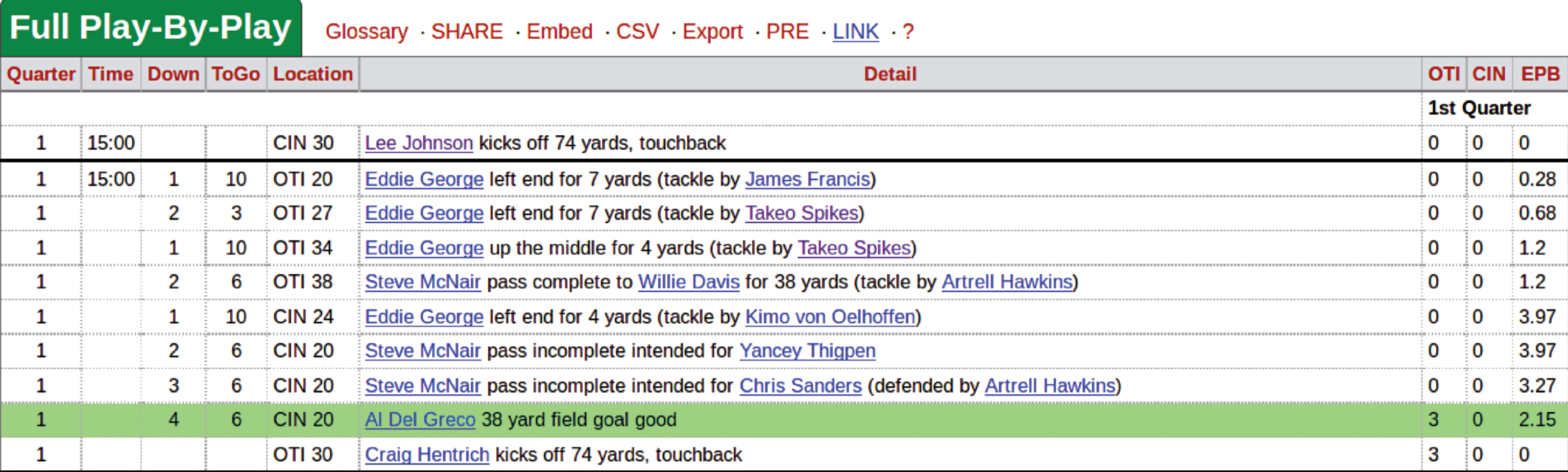
Outcomes were dichotomized as “good” or “not good”, the latter event includes blocks and fumbled holds. Our reasoning is that the blame for failed attempts usually rightly falls on the kicker, but sometimes the snap, the hold or the blocking are at fault. The records online do not easily allow for determination of blame. An example of an entry that was scraped from the url (http://www.pro-football-reference.com/boxscores/199809060cin.htm). (a game from week 1 of the 1998-1999 season) appears in Fig. 1.
Fig.1
Play-by-play item containing relevant information on a field goal attempt.
Occasionally, comparisons between total kick frequencies computed from play-by-play data with kicker career totals will reveal slight discrepancies, where certain plays are absent from the pro-football-reference play-by-play information. For example, in a 1998 Week 1 game of the New England Patriots at the Denver Broncos, Adam Vinatieri of the New England Patriots had a 37 yard field goal attempt during the second quarter. The pro-football-reference play-by-play account of the event is blank (see Fig. 2). We resorted to the site to attempt to rectify this particular record. Though we could not find links on the site to play-by-play information for games before 2001 (a situation in which automated screen-scraping is then difficult), we were able to find some urls, with links provided by a search engine.
Fig.2
Play-by-play item for a blocked kick by Adam Vinatieri in a 1998 Week 1 game that appeared as a blank on pro-football-reference.com
2.2Choice of a link function
For notation, we let k = 1, …, K index the kickers (K = 111 in our application) and let j = 1, …, N (N = 17104) index all of the field goal attempts. For each attempt, we let binary outcome Oj = 1 if the kick is good, and Oj = 0 otherwise. The probability of success of attempt j is denoted πj. The general form for the log-likelihood function of all of the probability parameters {πj} for independent, dichotomous data with outcomes oj is given by
Generalized linear models adopt a link function g, through which the probabilities πj are transformed to an expression that is linear in regression coefficients introduced to model the effects of available explanatory variables (and reduce the dimension of the parameter space). We define dj as the distance of the jth attempt and define indicator variables for kicker k as Xjk = I (jthattemptisbykicker k), for k = 1, …, K, with regression coefficients β1, …, βK. The probability parameters are now, after transformation by the link function g, linear in the regression coefficients,
We refer to βk as a kicker-specific slope and can test the significance of estimated regression coefficients by comparison with a generalized linear model with only one slope, β, to accommodate all kickers,
In applications in which statistical regression models are developed for binary response variables, logistic regression seems to be the most popular choice (Pasteur and Cunningham-Rhoads, 2014; Morris and Rolph, 1981; Bilder and Loughin, 1998; Berry and Wood, 2004), perhaps because of its interpretability, particularly through odds ratios. However, several other link functions are easily explored using statistical software for generalized linear models. We introduce a superscript notation for probability functions associated with kickers that will simplify the shrinkage estimation exposition in Section 3. Let πk (d) denote the success probability function for kicker k at any distance d. We consider three choices for the link function: logistic, probit, and CLL. Let Φ and Φ-1 denote the cumulative distribution function and quantile function, respectively, of a random variable with standard normal distribution. Then the links and inverse links (probability functions) for these three candidates are given below:
The log-likelihood function of a specified link function uses the reparameterizations above. As an example the log-likelihood for the logistic link is given by
Table 2 summarizes the maximized log-likelihood function when using the logit, probit, and CLL link functions for estimating field goal success probability in our data set. Tests comparing the nested models within a column of the table are all highly significant on 110 degrees of freedom (comparing models with K = 111 different slopes to a model with a single slope), indicating significant differences among the estimated slopes. With such a large sample, there does appear to be enough data to detect potentially subtle differences among kickers.
Table 2
Comparison of link functions: – 2 × maximized log-likelihood using full or restricted data set
| Link function | ||||
| Comp. | ||||
| Data | Model | Logit | Probit | log-log |
| All | Common slope | 14382 | 14365 | 14367 |
| Kicker-specific slopes | 14081 | 14062 | 14060 | |
| χ2 (df = 110) statistic | 301 | 303 | 307 | |
| Restricted to | Common slope | 11827 | 11820 | 11815 |
| 25 ≤ d ≤ 50 | Kicker-specific slopes | 11547 | 11535 | 11524 |
| χ2 (df = 110) statistic | 302 | 307 | 312 | |
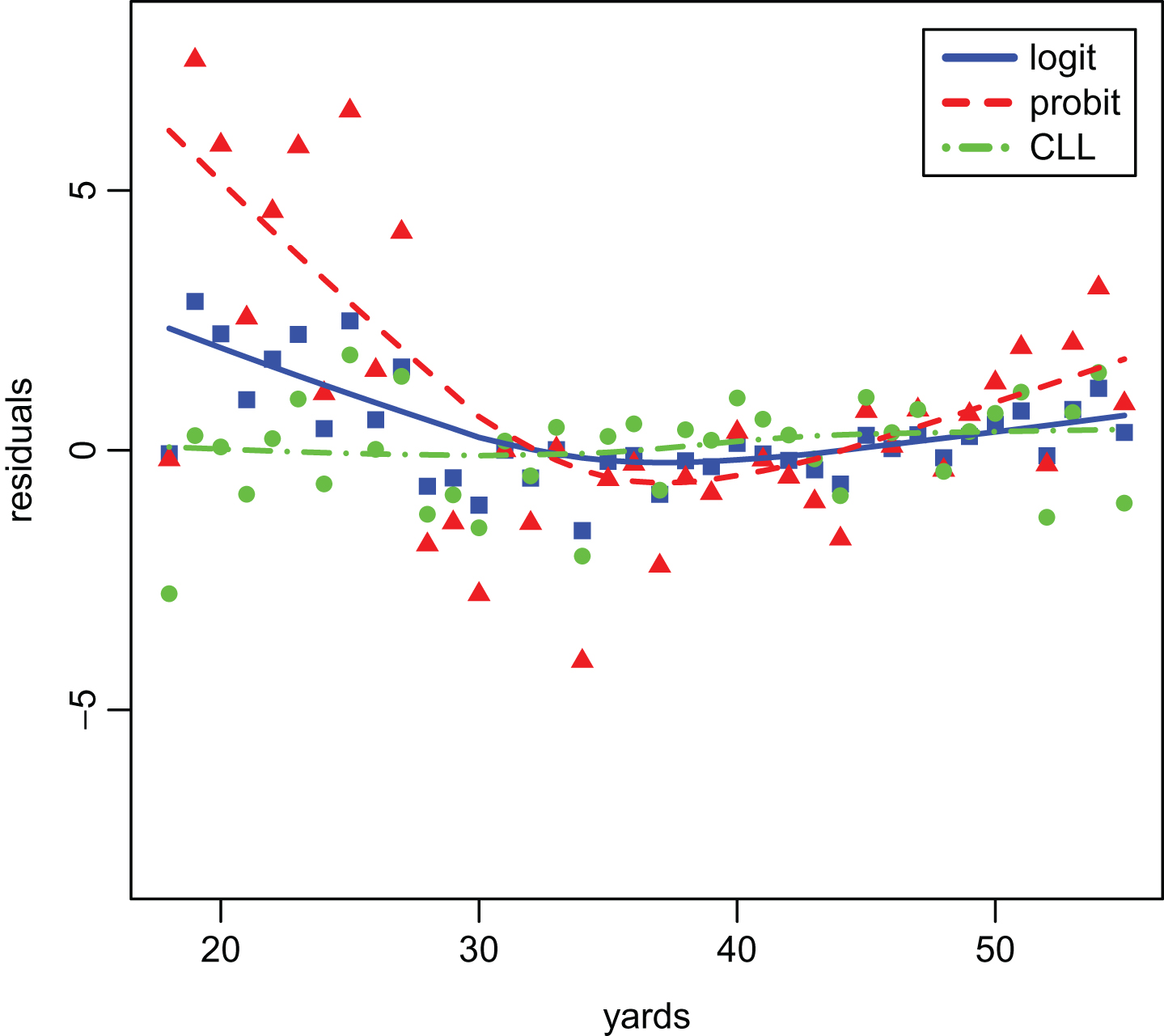
Figure 3 presents the inverse link functions applied to the empirical success frequencies against distance. The lines overlaid on the plots are from maximum likelihood estimation of the single-slope model. Residuals computed as standardized differences between transformed success frequencies and the estimated link functions are plotted against distances in Fig. 4, providing an enhanced visualization of the fits. Link-specific lowess smoothers overlaying these plots suggest that the residuals from the CLL fit exhibit the least dependence on distance.
Fig.3
The fits provided by three inverse link functions. Plot (a) presents the three fits to the empirical frequency data: logit link fit solid/blue, probit link dashed/red, complementary log-log link dot-dashed/green. Plots (b), (c) and (d) present the fits after link transformation. All four plots have distance in yards as the horizontal axis.
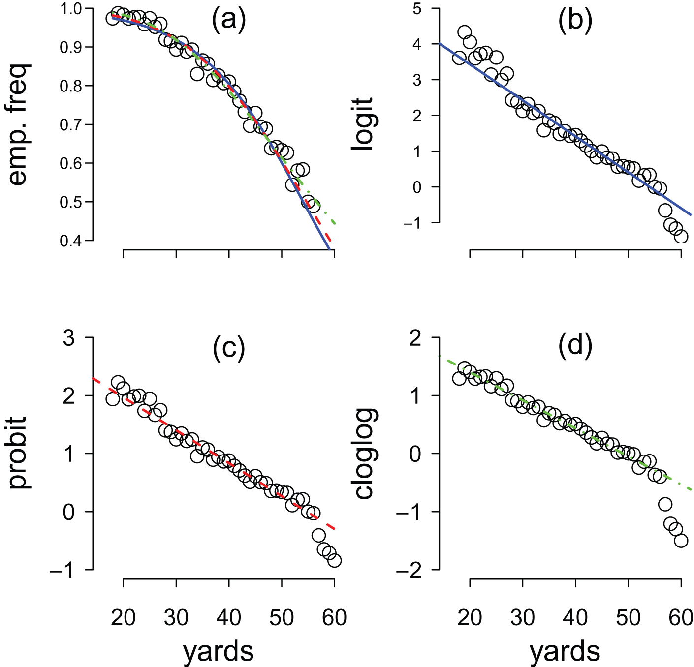
Fig.4
Residuals from three link functions in generalized linear models (logit as blue squares, probit as red triangles and complementary log-log as green circles). Residuals are differences from link-transformed empirical success frequencies and estimated link functions and have been normalized to have unit variance. Plotted against distances with at least 100 attempts, with Lowess smoothers overlaid using solid lines.
In an analytical comparison of link functions, McCullagh et al. (1989) observes that for trials with intermediate success probability, 0.1 ≤ π ≤ .9 (the vast majority of field goal attempts), probit and logistic functions are nearly linearly related, so that discrimination between the fits of models using these two links is difficult. Additionally, for trials with success probability approaching one (which occur as field goal attempt distances decrease towards 17 yards), the CLL approaches one more slowly than either of the other two link functions. The CLL link can also differ (Dobson and Barnett, 2011) from logit and probit links for small values of π, which are often of greatest interest when assessing kickers. Close inspection of Fig. 3 and Fig. 4 seem to reflect these observations, with better agreement with empirical frequencies on short kicks than that provided by either logit or probit. Fitting these models using kicks at the extremes may be problematic in that misses at short distances are likely due to mishandled snaps and attempts at long distances may lead to selection bias since these attempts are probably only afforded to very good kickers. In light of these issues, log-likelihood ratios are also reported after restricting attention to kicks with distances between 25 and 50 yards. With this restriction, the CLL link achieves the maximum likelihood among the link functions for models with either a single slope or with kicker-specific slopes.
The statistic proposed by Hosmer and Lemeshow (2004) (HL) offers another way to assess goodness-of-fit in regression models for binary data with continuous explanatory variables. The HL statistic is a Pearson-style measure of goodness-of-fit whose sampling distribution under a correctly specified model can be approximated by a chi-square distribution. The HL procedure partitions all kicks into 10 groups of roughly equal size. (We accomplished this using the algorithm laid out in the documentation for PROC LOGISTIC within the SAS statistical software package (SAS Institute, 2011). The procedure then computes, for each group, observed (Oi) and expected (Ei) counts of successful kicks by averaging estimated probabilities within group, in order to compute the χ2 statistic, X:
The summary statistics necessary for computation of the HL statistic are given in Table 3 for the logit and CLL links. The logistic regression model does not provide a good fit for the 10th group, where the estimated success probability is highest. The average estimated probability among these 1708 kicks is
Table 3
Summary statistics for Hosmer-Lemeshow assessment of the complementary log-log and logit link functions
| Complementary log-log link | Logit link | |||||||
| FG Made | FG Made | |||||||
| Group i | kicks, ni | oi | ei | χ2 | kicks, ni | oi | ei | χ2 |
| 1 | 1710 | 883 | 898.02 | 0.53 | 1711 | 871 | 842.32 | 1.92 |
| 2 | 1699 | 1112 | 1097.46 | 0.54 | 1712 | 1132 | 1104.61 | 1.91 |
| 3 | 1709 | 1217 | 1213.65 | 0.03 | 1715 | 1218 | 1241.27 | 1.58 |
| 4 | 1712 | 1315 | 1310.01 | 0.08 | 1705 | 1334 | 1336.55 | 0.02 |
| 5 | 1706 | 1387 | 1392.39 | 0.11 | 1710 | 1385 | 1425.98 | 7.09 |
| 6 | 1711 | 1473 | 1478.97 | 0.18 | 1712 | 1470 | 1500.63 | 5.06 |
| 7 | 1720 | 1565 | 1558.60 | 0.28 | 1709 | 1555 | 1555.20 | 0.00 |
| 8 | 1709 | 1604 | 1606.43 | 0.06 | 1709 | 1600 | 1598.85 | 0.01 |
| 9 | 1713 | 1655 | 1653.44 | 0.04 | 1713 | 1655 | 1635.25 | 5.26 |
| 10 | 1715 | 1685 | 1685.86 | 0.06 | 1708 | 1676 | 1655.34 | 8.37 |
| sum | 17104 | 13896 | 13894.83 | 1.89 | 17104 | 13896 | 13896.00 | 31.23 |
Table 4 gives HL chi-square statistics andp-values on 8 degrees of freedom for each of the three link functions with either a single slope, or with kicker-specific slopes. The models with the CLL link function are the only ones that do not exhibit significant lack-of-fit. With such a large sample size (N = 17, 104 attempts), even subtle lack-of-fit is likely to be detected, as in the logistic (p = .0291,. 0657) and probit (p < .0001, p = .0001) models. Despite this significance, neither of the two provides a bad fit.
Table 4
Hosmer-Lemeshow statistics and p-values for two models, each using the three different link functions
| Link function | ||||
| Data | Model | Logit | Probit | Comp log-log |
| All | Common slope | 34.1(<0.0001) | 17.1 (0.0291) | 8.9 (0.3489) |
| Kicker-specific slopes | 31.2 (0.0001) | 14.7 (0.0657) | 1.9 (0.9843) | |
| Restricted to | Common slope | 16.8(0.0329) | 11.6(0.1720) | 7.9(0.4463) |
| 25 ≤ d ≤ 50 | Kicker-specific slopes | 32.3(0.0001) | 24.1(0.0022) | 14.8(0.0630) |
| Restricted to | Common slope | 19.4(0.0130) | 12.4(0.1326) | 7.8(0.4508) |
| 25 ≤ d ≤ 55 | Kicker-specific slopes | 24.2(0.0021) | 16.3(0.0380) | 10.4(0.2383) |
Lastly, a link function could be chosen on the basis of how well probabilities estimated using the link can predict successful and unsuccessful field goal attempts. A decision rule which predicts a successful field goal when the estimated success probability exceeds some threshold (
Table 5
Area under the curve (AUC) for the three link functions
| Link function | |||
| Model | Logit | Probit | Comp log-log |
| Common slope | 0.7490 | – | – |
| Kicker-specific slopes | 0.7640 | 0.7641 | .7646 |
Since the CLL link enjoys the smallest HL and largest AUC under cross-validation (as described in Section 3.1), computations under the other two link functions are excluded from presentation in the remainder of the paper.
3Shrinkage estimation
Model-based estimates of kicker-specific success probabilities have large variance except in cases where the number of observed attempts for a given kicker is very large. As an example, consider interval estimation of the probability of success when kicking a 45 yard field goal using the CLL link function. For Adam Vinatieri, who has 572 career attempts, the 95% interval estimate is (0.69, 0.78). However, the 95% interval estimate of 45 yard field goal success probability for Garrett Hartley, who has 115 career attempts, is (0.59, 0.80), more than twice as wide as the interval estimate for Vinatieri. Estimators with reduced variance may be constructed by taking a weighted average of the kicker-specific maximum-likelihood estimator (MLE) and one developed for the average of all kickers. That is, the variance of an estimator may be reduced by shrinking it towards another estimator which has much lower variance.
Efron and Morris (1975) and Brown (2008) employed this method, viewed from an empirical Bayes perspective, to predict end-of-season batting averages in Major League Baseball. In particular, the papers propose shrinking hitter-specific estimates based on a small number of at-bats towards the early season batting average among all hitters. The methods are based on the theory James and Stein (1961) develops for estimation of the mean of a multivariate normal distribution. That theory does not apply directly to estimation of success probabilities for independent binary trials, as in field goal attempts, but the idea of variance-reduction is worth exploring.
Without any shrinkage, the kicker-specific MLE of the success probability at a given distance d is given by
The estimator with complete shrinkage is simply the empirical frequency of all kicks taken by all kickers at that distance,
These empirical frequencies are plotted in the top left graphic in Fig. 3.
3.1Proposed shrinkage estimators
For shrinkage estimators of the success probability at a given distance, π (d), we consider estimators that are weighted averages of the MLE and empirical frequency estimators defined above,
The first shrinkage estimator we propose is simply the midpoint between the two components. We refer to this shrinkage estimate, obtained by setting ω = 1/2, as the midpoint estimator (denoted by superscript M):
One approach towards constructing a shrinkage estimator that weights model-based kicker-specific estimates more heavily is simply to weight components in inverse proportion to their standard errors. This will upweight the MLE,
Note that because sample sizes differ, this weighting scheme can lead to different weights at different distances.
Another approach is to choose a weighting function for the MLE that is increasing in nk towards a maximum weight of one. Any cumulative distribution function (CDF) has this property. We choose the exponential distribution function, which for a suitably chosen rate parameter a, increases rapidly for small n with diminishing returns on large nk:
This choice leads to the exponentially weighted shrinkage estimator,
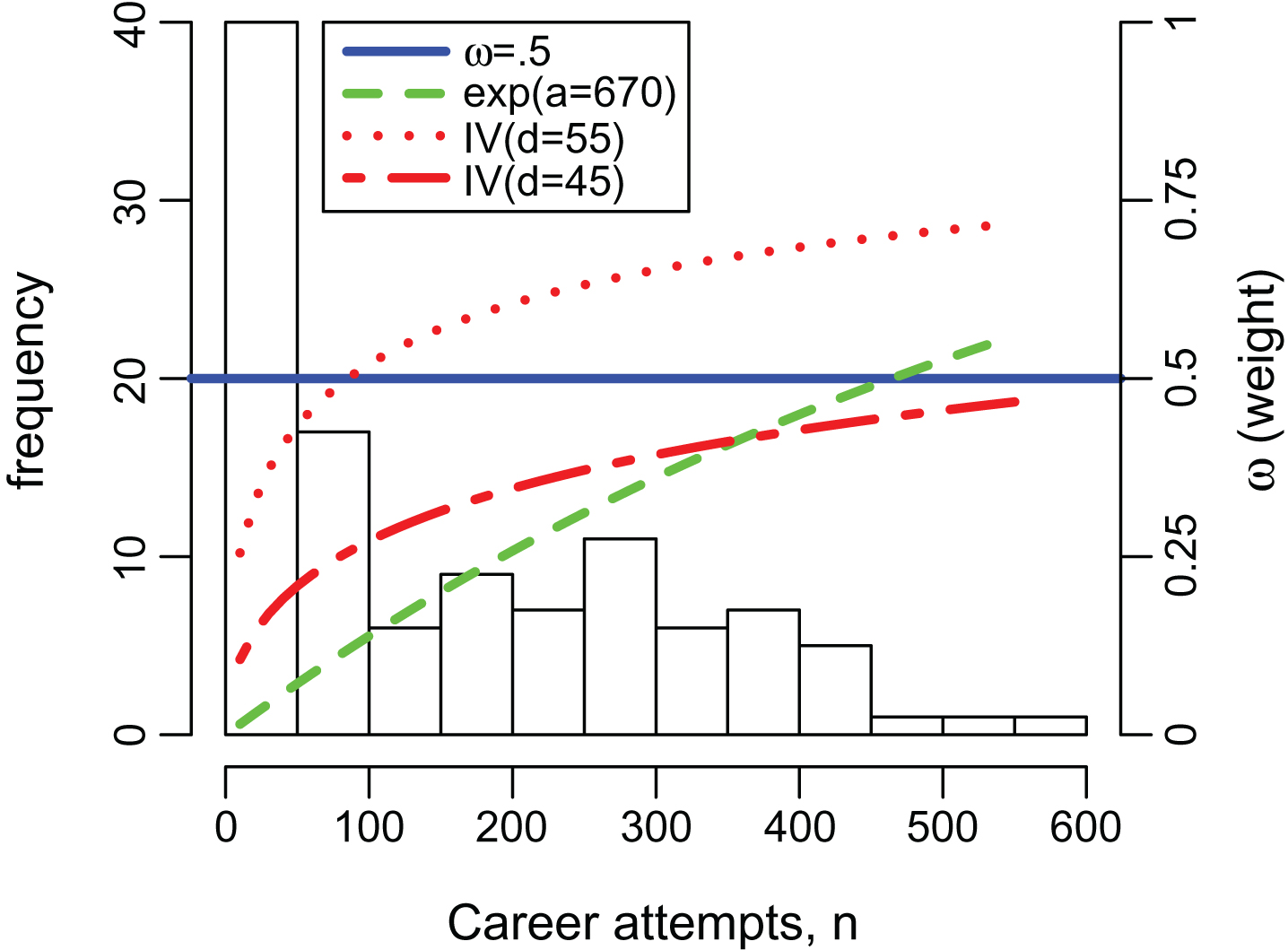
The quantity a in the exponential weights estimator can be viewed as a tuning parameter, whose value is “fit” using the entire dataset and whose performance is evaluated by cross-validation (see Section 3.2). For the a parameter, mean values 100 < a < 700 were considered, reasoning that the kick counts fell in the interval 4 < nk < 572. A search of values of a, to the nearest multiple of 10, achieves a Hosmer-Lemeshow (HL) statistic of HL = 9.32 at an optimized value of a = 670. Using the exponential CDF with mean a = 670 for a weight function, the corresponding weights on the model-based estimates for kickers with sample sizes of nk = 10, 50, 100, 200, 400 would be 0.02, 0.07, 0.14, 0.26, 0.45, respectively.
Figure 5 presents a plot of the weight function, ω for these different shrinkage estimators. The two separate curves provided for the IV weighted estimator corresponds to kicks at d = 45 and d = 55 yards. The empirical frequencies at these two distances were
Fig.5
Weight functions for shrinkage estimation, “exp” plots the weights based on the exponential distribution and IV plots the weights proportional to the inverse of the variances of the components.
The estimators of success probability can be naturally shrunk towards central values by means of a Bayesian generalized linear model with CLL link utilizing empirical Bayes estimation (see e.g.,Carlin and Louis (1997)). In such a model, as fit using the bayesglm function of the arm package in R (Gelman et al., 2014), the regression coefficients are assumed to be independent, normally distributed random variables with mean and variance characterized by hyper-parameters that are specified from data, in our case:
The hyperparameters for the intercept are the default choices for the bayesglm function and those for the kicker-specific slope were chosen from the sample mean and variance of maximum likelihood estimates from the frequentist generalized linear model fit.
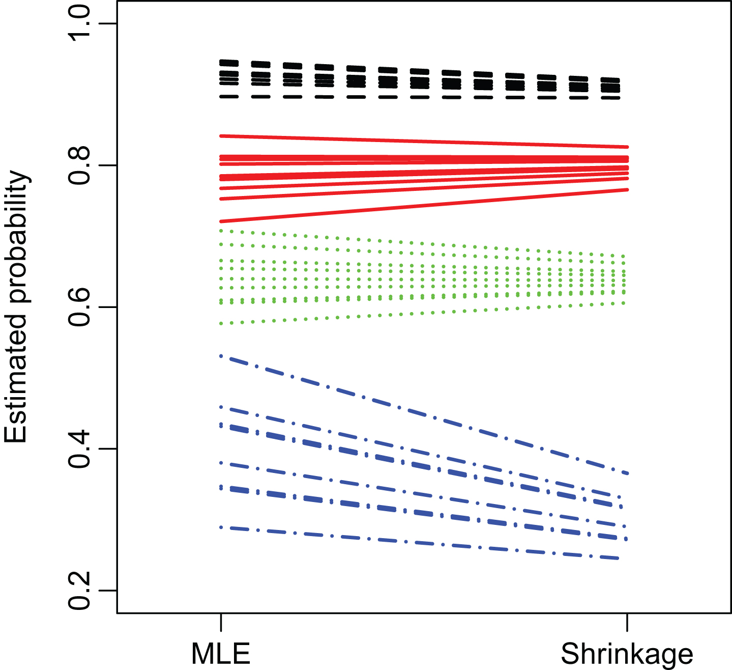
Fig. 7 illustrates the reduction in variance due to shrinkage. For attempt distances, d = 30, 40, 50, 60 yards, random samples of 10 kicks were selected. The estimated success probability estimates are plotted using different colors, with estimation technique on the horizontal axis. Not only is the reduction in variation apparent, but the model-based estimates at 60 yards are shifted downward. The explanation for this shift is lack-of-fit of the model for very long attempts. Shrinkage towards the empirical frequency tends to alleviate bias caused by this poor fit.
Fig.7
Model-based maximum-likelihood and shrinkage (midpoint) estimates of success probability, colored according to attempt distance (30, 40, 50, and 60 yards plotted with black, red,green and blue lines, respectively).
3.2Assessment using cross-validation
While HL is useful for quantifying how well several fitted models align with observed data, it may not tell the entire story as to how well the fitted model would generalize to observations made in the future, or out-of-sample data. Cross-validation (CV) can be used to quantify the degree to which a model fitted to observed data generalizes to data not used to fit the model or to compare the capacity of several models to generalize. Pasteur and Cunningham-Rhoads (2014) uses five-fold CV to select weather, pressure, and fatigue variables for a multiple logistic regression model. In five-fold CV, the dataset is partitioned into five subsets of equal size. The first subset is held out of the process where the model is fit, and then the fitted model is used to estimate the probabilities of the events that were held out. HL is then computed only for the held-out subset. This step is repeated four more times, holding out each subset exactly once. As can be seen from inspection of the first two numerical columns of Table 6, neither the model-based estimate (CLL) nor the empirical frequency (EF) generalize well under 5-fold CV, in the sense that there is disagreement between the number of observed and expected successful kicks when attempts are put into the 10 groups for the HL statistic. Recall that the midpoint estimated probability for any kick is simply the midpoint between CLL and EF. While this shrinkage estimate has a greater HL than its CLL and EF components when the entire dataset is used both to fit the model and to compute the goodness-of-fit statistic, it shows better agreement between observed and expected successful kicks under CV. The CV procedure was repeated four times, using four random partitions of the dataset into five subsets. Each time, the midpoint estimate enjoys a better fit for the held-out data than either of its two components, as quantified by the HL statistic. The shrinkage estimators based on the exponential weights, with a = 660, 670 or 680 also performed better than either component by itself. In computation of these estimates, the step of tuning the a “parameter” was not repeated during cross-validation. Rather, estimates based on values of a = 660, 670, 680 (which did the best on the entire dataset) were computed for every observation, and only those results are reported here. If this weighting scheme is tolerable, then it appears to perform comparably to the simple midpoint shrinkage estimator. Among the six estimators reported in Table 6, there is no dominant choice when considering performance under cross-validation. One clear observation, however, is that the midpoint and exponential shrinkage estimators are generalizing to out-of-sample data better than either the CLL or EF components by themselves.
Table 6
Hosmer-Lemeshow statistics under 5-fold cross-validation for the estimators
| Shrinkage | 5-fold Cross Validation | |||||
| Estimator | All Data | 1x | 2x | 3x | 4x | CV avg |
| CLL | 1.89 | 15.60 | 20.13 | 22.59 | 22.13 | 20.12 |
| EF | 0.00 | 8.96 | 25.25 | 19.45 | 13.14 | 16.70 |
| midpoint | 11.87 | 8.70 | 9.57 | 5.29 | 4.68 | 7.06 |
| exp(a=660) | 9.83 | 6.97 | 10.03 | 4.19 | 9.07 | 7.56 |
| exp(a=670) | 9.32 | 7.05 | 10.52 | 4.23 | 9.21 | 7.75 |
| exp(a=680) | 9.93 | 7.16 | 10.20 | 4.81 | 7.73 | 7.47 |
| IV | 12.69 | 16.30 | 33.70 | 19.12 | 18.50 | 21.90 |
| Bayesian CLL | 19.08 | 29.03 | 10.72 | 11.94 | 17.72 | 17.35 |
4Applications
4.1Ranking kickers
In addition to estimating the success probability for a given kicker from a given distance, the estimation methodology can be used to rank NFL kickers. Historically, comparisons among kickers in sports media have been made using the overall number (as on espn.go.com) or proportion of successful attempts (as on sports.yahoo.com or si.com) without regard to distance, as it not obvious how to incorporate distance and degree of difficulty based on summary statistics. Alternatively, Berry and Berry (1985) suggests averaging model-based kicker-specific estimates over the league-wide distribution of attempt distances. A histogram for these attempts is given in Fig. 8. The average distance over all 17, 104 attempts was 36.6 yards. Tables 7, 8, and 9 present a ranking of kickers under this summary statistic, using several different methods of estimation, along with the standard “overall” metric.
Fig.8
Frequency histogram of attempt distances.
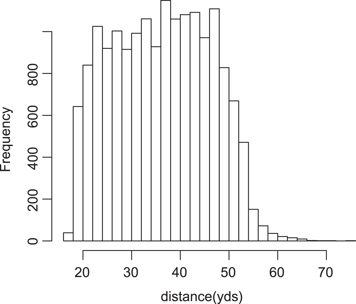
Table 7
Kicker ranking by shrinkage estimate over distribution of all kicks. The columns include the average attempt distance, actual success frequencies for kicks of less than 40 yards, 40-49 yards, and at least 50 yards, overall proportion of successful field goal attempts, ranking by overall success proportion, kicker-specific MLE (
| Kicker | avg attempt | <40 | 40 - 49 | ≥50 | pct | rank |
|
|
| Justin Tucker | 38.11 | 64/65 | 26/30 | 15/21 | 0.91 | 1 | 0.92 | 0.87 |
| Dan Bailey | 38.71 | 63/66 | 35/39 | 17/25 | 0.88 | 3 | 0.90 | 0.86 |
| Chandler Catanzaro | 38.21 | 17/19 | 10/11 | 2/3 | 0.88 | 5 | 0.89 | 0.85 |
| Kai Forbath | 36.90 | 35/38 | 22/25 | 2/4 | 0.88 | 4 | 0.88 | 0.85 |
| Blair Walsh | 39.01 | 53/57 | 19/24 | 17/24 | 0.85 | 17 | 0.88 | 0.84 |
| Connor Barth | 38.52 | 65/69 | 42/51 | 13/20 | 0.86 | 11 | 0.87 | 0.84 |
| Cody Parkey | 35.42 | 24/26 | 4/6 | 4/4 | 0.89 | 2 | 0.87 | 0.84 |
| Patrick Murray | 41.08 | 9/11 | 6/7 | 5/6 | 0.83 | 27.5 | 0.87 | 0.84 |
| Dan Carpenter | 38.03 | 111/115 | 65/82 | 20/34 | 0.85 | 16 | 0.87 | 0.84 |
| Steven Hauschka | 36.45 | 95/100 | 40/49 | 9/17 | 0.87 | 8 | 0.86 | 0.84 |
| Greg Zuerlein | 39.96 | 43/48 | 17/19 | 13/22 | 0.82 | 39 | 0.86 | 0.84 |
| Robbie Gould | 36.55 | 164/173 | 74/100 | 17/23 | 0.86 | 9 | 0.86 | 0.84 |
| Rob Bironas | 37.62 | 147/158 | 71/92 | 24/35 | 0.85 | 15 | 0.86 | 0.84 |
| Jason Hanson | 38.31 | 210/223 | 108/141 | 43/68 | 0.84 | 23 | 0.86 | 0.83 |
| John Kasay | 37.32 | 198/203 | 88/114 | 32/63 | 0.84 | 22 | 0.85 | 0.83 |
| Stephen Gostkowski | 35.08 | 185/201 | 65/85 | 14/18 | 0.87 | 7 | 0.85 | 0.83 |
| Josh Brown | 37.72 | 185/196 | 81/111 | 35/54 | 0.83 | 25 | 0.85 | 0.83 |
| Matt Bryant | 35.91 | 200/214 | 73/95 | 20/34 | 0.85 | 12 | 0.85 | 0.83 |
| Mike Vanderjagt | 35.85 | 157/167 | 71/95 | 15/23 | 0.85 | 13 | 0.84 | 0.83 |
| Matt Stover | 34.96 | 236/247 | 97/131 | 9/20 | 0.86 | 10 | 0.84 | 0.83 |
| Jeff Hall | 39.60 | 2/2 | 1/2 | 1/1 | 0.80 | 54.5 | 0.84 | 0.82 |
| Shayne Graham | 35.29 | 197/211 | 69/89 | 15/30 | 0.85 | 14 | 0.83 | 0.82 |
| Sebastian Janikowski | 38.99 | 222/239 | 111/148 | 48/88 | 0.80 | 53 | 0.83 | 0.82 |
| Phil Dawson | 35.65 | 256/280 | 85/115 | 35/51 | 0.84 | 19 | 0.83 | 0.82 |
| Adam Vinatieri | 35.80 | 322/354 | 135/173 | 26/45 | 0.84 | 18 | 0.83 | 0.82 |
| Jeff Wilkins | 37.35 | 166/177 | 67/100 | 28/41 | 0.82 | 38 | 0.83 | 0.82 |
| Joe Nedney | 36.77 | 154/163 | 62/88 | 17/31 | 0.83 | 35 | 0.83 | 0.82 |
| Ryan Longwell | 36.68 | 228/248 | 97/133 | 24/40 | 0.83 | 32 | 0.83 | 0.82 |
| Josh Scobee | 38.15 | 142/153 | 74/106 | 26/42 | 0.80 | 50 | 0.83 | 0.82 |
| Gary Anderson | 35.70 | 105/114 | 56/74 | 3/7 | 0.84 | 20 | 0.82 | 0.82 |
| Ryan Succop | 37.03 | 88/96 | 43/58 | 12/20 | 0.82 | 36 | 0.82 | 0.82 |
| Shaun Suisham | 35.98 | 142/157 | 76/94 | 6/18 | 0.83 | 30 | 0.82 | 0.82 |
| Randy Bullock | 38.66 | 34/37 | 19/25 | 5/11 | 0.79 | 57 | 0.82 | 0.82 |
| Nate Kaeding | 35.46 | 129/135 | 51/73 | 10/19 | 0.84 | 21 | 0.82 | 0.82 |
| Garrett Hartley | 35.12 | 62/73 | 28/34 | 6/8 | 0.83 | 24 | 0.81 | 0.81 |
| Jay Feely | 36.40 | 232/259 | 95/130 | 19/34 | 0.82 | 41 | 0.81 | 0.81 |
| Nick Folk | 37.33 | 128/142 | 57/78 | 19/34 | 0.80 | 52 | 0.81 | 0.81 |
Table 8
Ranking by shrinkage estimate over distribution of all kicks, continued
| Kicker | avg attempt | <40 | 40 - 49 | ≥50 | pct | rank |
|
|
| Mason Crosby | 37.47 | 155/168 | 56/76 | 23/50 | 0.80 | 56 | 0.81 | 0.81 |
| Jason Elam | 36.85 | 200/214 | 93/130 | 26/42 | 0.83 | 34 | 0.81 | 0.81 |
| Nick Novak | 36.81 | 81/92 | 31/41 | 12/20 | 0.81 | 47 | 0.81 | 0.81 |
| John Carney | 35.25 | 213/236 | 77/108 | 11/18 | 0.83 | 31 | 0.81 | 0.81 |
| Mike Nugent | 36.42 | 132/145 | 57/76 | 10/24 | 0.81 | 43 | 0.81 | 0.81 |
| Alex Henery | 36.07 | 52/57 | 22/29 | 3/8 | 0.82 | 40 | 0.81 | 0.81 |
| Matt Prater | 37.92 | 107/115 | 43/66 | 25/35 | 0.81 | 48 | 0.81 | 0.81 |
| Cairo Santos | 35.10 | 17/18 | 7/10 | 1/2 | 0.83 | 27.5 | 0.81 | 0.81 |
| David Akers | 36.34 | 292/318 | 110/159 | 27/52 | 0.81 | 45 | 0.81 | 0.81 |
| Doug Brien | 36.93 | 80/90 | 48/61 | 7/17 | 0.80 | 51 | 0.81 | 0.81 |
| Rian Lindell | 36.09 | 209/226 | 75/111 | 23/42 | 0.81 | 49 | 0.80 | 0.81 |
| Al Del Greco | 35.61 | 48/52 | 20/30 | 1/2 | 0.82 | 37 | 0.80 | 0.81 |
| Jeff Reed | 34.94 | 169/183 | 54/79 | 8/17 | 0.83 | 33 | 0.80 | 0.81 |
| Graham Gano | 37.27 | 77/89 | 40/54 | 12/20 | 0.79 | 59 | 0.80 | 0.81 |
| Caleb Sturgis | 37.72 | 36/39 | 14/20 | 6/13 | 0.78 | 61.5 | 0.80 | 0.81 |
| Neil Rackers | 37.10 | 183/203 | 68/95 | 26/53 | 0.79 | 60 | 0.80 | 0.80 |
| Jay Taylor | 34.67 | 3/4 | 1/1 | 1/1 | 0.83 | 27.5 | 0.80 | 0.80 |
| Olindo Mare | 35.54 | 238/267 | 89/117 | 19/41 | 0.81 | 42 | 0.80 | 0.80 |
| Morten Andersen | 35.73 | 136/150 | 53/77 | 8/16 | 0.81 | 46 | 0.79 | 0.80 |
| David Buehler | 38.15 | 13/16 | 8/11 | 4/6 | 0.76 | 72 | 0.79 | 0.80 |
| Mike Hollis | 35.89 | 85/98 | 36/51 | 7/11 | 0.80 | 54.5 | 0.79 | 0.80 |
| Clint Stitser | 30.75 | 6/7 | 1/1 | 0/0 | 0.88 | 6 | 0.78 | 0.80 |
| Paul Edinger | 38.40 | 74/92 | 49/68 | 16/24 | 0.76 | 73 | 0.78 | 0.80 |
| Martin Gramatica | 37.20 | 114/128 | 37/63 | 19/29 | 0.77 | 63 | 0.78 | 0.80 |
| Lawrence Tynes | 34.80 | 153/173 | 42/60 | 11/21 | 0.81 | 44 | 0.78 | 0.80 |
| Norm Johnson | 37.00 | 28/32 | 17/22 | 1/6 | 0.77 | 68 | 0.77 | 0.79 |
| Kris Brown | 37.02 | 167/194 | 76/111 | 18/35 | 0.77 | 67 | 0.77 | 0.79 |
| Todd Peterson | 35.56 | 113/131 | 43/59 | 8/17 | 0.79 | 58 | 0.77 | 0.79 |
| Pete Stoyanovich | 36.21 | 36/40 | 15/26 | 3/4 | 0.77 | 64.5 | 0.77 | 0.79 |
| Billy Cundiff | 36.39 | 136/156 | 52/73 | 9/29 | 0.76 | 69 | 0.76 | 0.79 |
| John Hall | 36.99 | 128/144 | 51/84 | 10/23 | 0.75 | 74 | 0.76 | 0.79 |
| Brett Conway | 36.30 | 49/59 | 20/27 | 5/11 | 0.76 | 70 | 0.76 | 0.78 |
| Bill Gramatica | 35.69 | 25/27 | 10/15 | 2/6 | 0.77 | 66 | 0.76 | 0.78 |
| Cary Blanchard | 37.44 | 29/34 | 13/21 | 3/6 | 0.74 | 78 | 0.75 | 0.78 |
| Steve Christie | 35.25 | 105/121 | 35/59 | 10/17 | 0.76 | 71 | 0.74 | 0.78 |
| Dave Rayner | 37.41 | 42/51 | 19/29 | 5/11 | 0.73 | 81 | 0.74 | 0.78 |
| Chris Jacke | 37.27 | 25/28 | 6/11 | 1/5 | 0.73 | 80 | 0.74 | 0.77 |
| John Potter | 34.75 | 2/2 | 1/1 | 0/1 | 0.75 | 75.5 | 0.73 | 0.77 |
| Todd France | 33.78 | 5/5 | 2/4 | 0/0 | 0.78 | 61.5 | 0.73 | 0.77 |
| Brad Daluiso | 33.76 | 40/46 | 13/23 | 1/1 | 0.77 | 64.5 | 0.72 | 0.77 |
| Craig Hentrich | 48.50 | 2/2 | 2/3 | 1/5 | 0.50 | 104.5 | 0.72 | 0.77 |
| Cedric Oglesby | 30.00 | 4/5 | 1/1 | 0/0 | 0.83 | 27.5 | 0.72 | 0.76 |
Table 9
Ranking by shrinkage estimate over distribution of all kicks, continued
| Kicker | avg attempt | <40 | 40 - 49 | ≥50 | pct | rank |
|
|
| Richie Cunningham | 35.03 | 35/43 | 12/18 | 1/4 | 0.74 | 77 | 0.71 | 0.76 |
| Jeff Chandler | 34.60 | 16/18 | 6/10 | 0/2 | 0.73 | 79 | 0.70 | 0.76 |
| Wade Richey | 35.36 | 58/69 | 19/35 | 3/7 | 0.72 | 82 | 0.70 | 0.75 |
| Tim Seder | 35.95 | 30/36 | 14/23 | 0/3 | 0.71 | 84 | 0.70 | 0.75 |
| Aaron Elling | 36.75 | 14/17 | 4/7 | 1/4 | 0.68 | 90 | 0.68 | 0.75 |
| Eddie Murray | 35.65 | 12/14 | 4/8 | 0/1 | 0.70 | 86 | 0.68 | 0.75 |
| Doug Pelfrey | 35.98 | 29/36 | 7/15 | 3/6 | 0.68 | 88 | 0.67 | 0.74 |
| Taylor Mehlhaff | 32.75 | 2/3 | 1/1 | 0/0 | 0.75 | 75.5 | 0.67 | 0.74 |
| Michael Husted | 35.93 | 32/44 | 14/21 | 1/4 | 0.68 | 89 | 0.66 | 0.74 |
| Brian Gowins | 35.83 | 3/3 | 1/2 | 0/1 | 0.67 | 93.5 | 0.66 | 0.73 |
| Jose Cortez | 34.07 | 41/50 | 11/24 | 1/1 | 0.71 | 85 | 0.65 | 0.73 |
| Steve Lindsey | 32.71 | 3/5 | 2/2 | 0/0 | 0.71 | 83 | 0.65 | 0.73 |
| Greg Davis | 36.68 | 11/15 | 6/11 | 1/2 | 0.64 | 97 | 0.64 | 0.73 |
| Jeff Jaeger | 34.85 | 19/23 | 2/9 | 2/2 | 0.68 | 91 | 0.64 | 0.73 |
| Jon Hilbert | 37.39 | 9/10 | 2/8 | 0/0 | 0.61 | 99 | 0.63 | 0.72 |
| Kris Heppner | 35.00 | 8/11 | 2/2 | 0/2 | 0.67 | 93.5 | 0.63 | 0.72 |
| Justin Medlock | 34.83 | 6/7 | 2/4 | 0/1 | 0.67 | 93.5 | 0.63 | 0.72 |
| Chris Boniol | 35.30 | 19/24 | 6/14 | 1/2 | 0.65 | 96 | 0.63 | 0.72 |
| Brandon McManus | 34.85 | 7/8 | 2/3 | 0/2 | 0.69 | 87 | 0.62 | 0.72 |
| Jake Arians | 37.90 | 8/10 | 4/11 | 0/0 | 0.57 | 102 | 0.61 | 0.71 |
| Seth Marler | 35.88 | 14/19 | 5/12 | 1/2 | 0.61 | 100 | 0.59 | 0.70 |
| James Tuthill | 35.06 | 7/10 | 2/5 | 1/1 | 0.63 | 98 | 0.59 | 0.70 |
| Ola Kimrin | 36.40 | 5/6 | 1/3 | 0/1 | 0.60 | 101 | 0.59 | 0.70 |
| Ricky Schmitt | 33.33 | 2/3 | 0/0 | 0/0 | 0.67 | 93.5 | 0.59 | 0.70 |
| Owen Pochman | 41.59 | 4/9 | 4/5 | 0/3 | 0.47 | 106 | 0.58 | 0.69 |
| Hayden Epstein | 35.33 | 5/6 | 0/2 | 0/1 | 0.56 | 103 | 0.52 | 0.67 |
| Nate Freese | 38.14 | 3/3 | 0/4 | 0/0 | 0.43 | 107 | 0.45 | 0.63 |
| Shane Andrus | 38.20 | 2/3 | 0/2 | 0/0 | 0.40 | 108 | 0.45 | 0.63 |
| Michael Koenen | 44.00 | 2/5 | 0/1 | 2/8 | 0.29 | 111 | 0.45 | 0.63 |
| Scott Blanton | 39.33 | 1/2 | 0/1 | 0/0 | 0.33 | 109.5 | 0.42 | 0.62 |
| Aaron Pettrey | 29.25 | 2/3 | 0/1 | 0/0 | 0.50 | 104.5 | 0.32 | 0.56 |
| Toby Gowin | 34.67 | 1/2 | 0/1 | 0/0 | 0.33 | 109.5 | 0.30 | 0.56 |
For veteran kickers with a large number of kicks that are similar in distribution to that of the whole league, the effect of shrinkage is minimal. Adam Vinatieri has succeeded on 84% of 572 attempted kicks at an average distance of 35.8. His model-based estimate averaged over the distribution of all NFL kicks in 1998-2014 is 0.83 and the shrinkage estimate is only slightly different at 0.82. Conversely kickers like Patrick Murray and Greg Zuerlein have achieved very successful records so far in their young careers, hitting 20/24 (83%) and 73/89 (82%), at longer-than-average average distances of 41.1 yards and 40.0 yards respectively. Their model-based estimates averaged over the league-wide distribution of distances is more favorable (87% and 86%; note the bump up in rank from that based on the empirical frequency) but the shrinkage estimate brings these closer to more average kickers (84% for both kickers).
These tables suggest a ranking that places many current kickers among the best over the last 16 year period. Justin Tucker has been successful on 105 out of 116 attempts, with average distance
4.2Stadium effects
A topic of interest for many fans, writers and announcers is the effects of certain stadiums on the chances of making a field goal. The open end of Heinz Field receives particular attention for increased difficulty due to wind (Batista, 2002). Modeling fixed factorial effects for stadiums enables investigation of this issue. Though a likelihood ratio test finds evidence of stadium effects (χ2 = 112, p < 0.0001, df = 50), their inclusion does not lead to an improved fit as assessed by Hosmer-Lemeshow, where there is a greater discrepancy between observed and expected counts than the model based on kickers and distances alone (HL = 8.3with stadium effects and HL = 1.9 without stadium effects, from Table 3). Nevertheless, including these effects does help to identify the more difficult and more favorable stadiums in which to kick, though again the estimation may suffer from selectionbias.
Success probabilities for each stadium can be estimated by back-transforming the marginal mean on the CLL scale. These marginal means average equally over all kickers and correspond to the average distance of
Table 11
Stadium effects and success frequencies. The columns include number of games, average
distance, attempts per game, empirical success rates as counts and as a percentage and model-based success probability estimate (
| Franchise | Stadium | games |
| att/g | made/att | pct |
| Std.err. |
| Colts | Lucas Oil Stadium | 62 | 37.4 | 3.9 | 217/244 | 0.89 | 0.88 | 0.03 |
| Lions | Pontiac Silverdome | 32 | 38.2 | 4.0 | 109/127 | 0.86 | 0.87 | 0.04 |
| Broncos | Sports Authority Field at Mile High | 119 | 37.9 | 3.7 | 375/442 | 0.85 | 0.84 | 0.02 |
| Vikings | Mall of America Field | 131 | 37.0 | 3.7 | 408/483 | 0.84 | 0.84 | 0.02 |
| Lions | Ford Field | 107 | 38.1 | 3.8 | 344/406 | 0.85 | 0.83 | 0.02 |
| Giants/Jets | MetLife Stadium | 82 | 36.4 | 3.8 | 270/313 | 0.86 | 0.83 | 0.03 |
| Ravens | M&T Bank Stadium | 141 | 36.2 | 4.1 | 494/572 | 0.86 | 0.83 | 0.02 |
| Cowboys | Texas Stadium | 90 | 37.0 | 3.8 | 267/342 | 0.78 | 0.82 | 0.03 |
| Eagles | Lincoln Financial Field | 103 | 36.0 | 3.7 | 324/383 | 0.85 | 0.81 | 0.03 |
| Rams | The Dome at America’s Center | 140 | 38.6 | 3.9 | 454/551 | 0.82 | 0.80 | 0.02 |
| Saints | Mercedes-Benz Superdome | 134 | 36.6 | 3.7 | 410/492 | 0.83 | 0.80 | 0.02 |
| Cowboys | AT&T Stadium | 51 | 37.6 | 3.8 | 167/196 | 0.85 | 0.79 | 0.04 |
| Texans | NRG Stadium | 107 | 37.8 | 3.8 | 327/403 | 0.81 | 0.79 | 0.03 |
| Falcons | Georgia Dome | 141 | 36.4 | 3.7 | 433/525 | 0.82 | 0.79 | 0.02 |
| Panthers | Bank of America Stadium | 140 | 36.8 | 3.7 | 425/519 | 0.82 | 0.78 | 0.02 |
| Eagles | Veterans Stadium | 44 | 36.5 | 3.8 | 131/167 | 0.78 | 0.78 | 0.04 |
| Seahawks | CenturyLink Field | 114 | 36.6 | 3.8 | 361/433 | 0.83 | 0.78 | 0.03 |
| Cardinals | Sun Devil Stadium | 64 | 38.0 | 3.6 | 173/231 | 0.75 | 0.78 | 0.03 |
| Chiefs | Arrowhead Stadium | 138 | 36.7 | 3.9 | 435/543 | 0.80 | 0.77 | 0.02 |
| Chargers | Qualcomm Stadium | 141 | 35.9 | 3.7 | 427/525 | 0.81 | 0.77 | 0.02 |
| Buccaneers | Raymond James Stadium | 140 | 37.3 | 3.7 | 417/515 | 0.81 | 0.77 | 0.02 |
| Dolphins | Hard Rock Stadium | 142 | 36.9 | 4.1 | 470/579 | 0.81 | 0.77 | 0.02 |
| Jaguars | EverBank Field | 114 | 37.3 | 3.6 | 323/410 | 0.79 | 0.77 | 0.03 |
| Colts | RCA Dome | 87 | 36.0 | 4.0 | 282/345 | 0.82 | 0.76 | 0.03 |
| 49ers | Candlestick Park | 132 | 35.8 | 3.8 | 403/500 | 0.81 | 0.76 | 0.02 |
| Bengals | Paul Brown Stadium | 123 | 36.0 | 3.8 | 375/462 | 0.81 | 0.74 | 0.03 |
| Patriots | Gillette Stadium | 120 | 35.3 | 3.7 | 364/441 | 0.83 | 0.74 | 0.03 |
| Giants/Jets | Giants Stadium | 199 | 34.9 | 3.7 | 594/740 | 0.80 | 0.74 | 0.02 |
| Raiders | Oakland-Alameda County Coliseum | 140 | 37.8 | 4.1 | 441/573 | 0.77 | 0.74 | 0.02 |
| Titans | Nissan Stadium | 132 | 36.8 | 3.8 | 400/498 | 0.80 | 0.74 | 0.03 |
| Bills | New Era Field | 129 | 35.3 | 3.9 | 403/504 | 0.80 | 0.74 | 0.03 |
| Packers | Lambeau Field | 146 | 36.4 | 3.8 | 431/548 | 0.79 | 0.73 | 0.03 |
| Cardinals | University of Phoenix Stadium | 77 | 36.8 | 4.0 | 248/311 | 0.80 | 0.73 | 0.03 |
| Patriots | Foxboro Stadium | 33 | 35.6 | 4.3 | 111/143 | 0.78 | 0.73 | 0.04 |
| Steelers | Heinz Field | 123 | 35.9 | 3.6 | 350/445 | 0.79 | 0.72 | 0.03 |
| Browns | FirstEnergy Stadium | 128 | 35.1 | 3.8 | 388/482 | 0.80 | 0.71 | 0.03 |
| Redskins | FedExField | 138 | 36.3 | 3.7 | 390/514 | 0.76 | 0.71 | 0.02 |
| Bears | Soldier Field | 134 | 35.9 | 3.7 | 382/495 | 0.77 | 0.69 | 0.03 |
The ranking in Table 11 seems to corroborate the anecdote that Heinz Field is a tough place to kick, as does the lower-than-average distance of field goal attempts. The new stadium in Denver, “Sports Authority Field at Mile High,” also has a reputation as a good place to kick and it does turn up high on this list. The estimates based on marginal means also tend to be lower than the empirical success rates. This observation may possibly be due to the fact that marginal means average equally over all kickers. Empirical success rates will tend to involve more attempts from high-frequency kickers, who tend to be better kickers.
4.3Big legs
The capacity to kick long-distance field goals is of particular interest to many football fans as well as NFL team management. One way to enrich the model to allow rankings among kickers to vary across distance is to expand the degree of the polynomial to quadratic. Using L and Q superscripts for the linear and quadratic kicker effects leads to the following representations of the generalized linearmodel:
For this investigation, attention is restricted to the K′ = 54 veteran kickers with at least 100 attempts in their careers, since small sample sizes present greater separability issues for fitting quadratic models. A comparison of the model with kicker-specific slopes nested within the quadratic model is not significant using this restricted dataset (χ2 = 63.3, df = 54, p = 0.181). This non-significance could possibly be explained by selection bias, as kickers with many attempts will all tend to be good enough to remain in the league. While not significant, there is a preponderance of kickers for whom the estimated quadratic coefficients have small p-values, suggesting that there are some kickers for whom quadratic coefficients are non-zero. In fact the average p-value for these 54 tests of the form
Table 10 enables simultaneous inspection of kickers who have estimated success probabilities that rank highly (top 20) in at least one of the three distances, 35, 45 or 55 yards. Entries in the table are sorted by the success probability estimate at 55 yards,
Fig.6
Three clusters of kickers using shrinkage estimates of success probabilities at three distances.
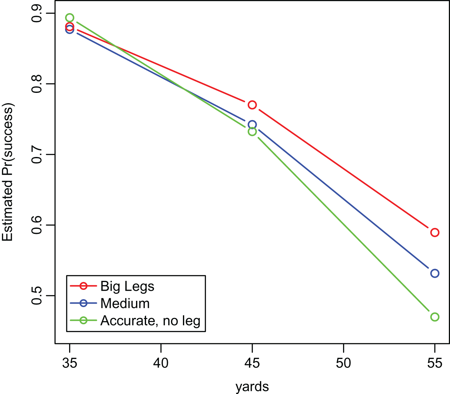
Table 10
Rankings of kickers among the top 20 at three different distances: 35, 45, and 55 yards. The columns include career span within the data set, ranks at each of the three distances, success probability shrinkage estimate at each of the three distances, and the empirical success probability at three distance ranges 30-39, 40-49, and 50-59 yards. Dashed lines separate clusters
| career | ranks |
| empirical success | |||||||
| Kicker | span | d = 35 | 45 | 55 | 35 | 45 | 55 | 30 - 39 | 40 - 49 | 50 - 59 |
| Garrett Hartley | 08-14 | 46 | 11 | 1 | 0.85 | 0.75 | 0.62 | 27/35 | 28/34 | 6/8 |
| Dan Bailey | 11-14 | 3 | 2 | 2 | 0.91 | 0.80 | 0.60 | 38/40 | 35/39 | 17/25 |
| Justin Tucker | 12-14 | 1 | 1 | 3 | 0.92 | 0.81 | 0.60 | 32/33 | 26/30 | 14/19 |
| Paul Edinger | 00-05 | 53 | 38 | 4 | 0.82 | 0.72 | 0.59 | 35/51 | 49/68 | 16/24 |
| Stephen Gostkowski | 06-14 | 22 | 8 | 5 | 0.88 | 0.76 | 0.59 | 94/105 | 65/85 | 14/18 |
| Blair Walsh | 12-14 | 9 | 3 | 6 | 0.89 | 0.78 | 0.58 | 30/33 | 19/24 | 17/23 |
| Connor Barth | 08-14 | 7 | 4 | 7 | 0.90 | 0.77 | 0.57 | 33/37 | 42/51 | 13/20 |
| Rob Bironas | 05-13 | 15 | 6 | 8 | 0.88 | 0.76 | 0.57 | 75/83 | 71/92 | 23/31 |
| Phil Dawson | 99-14 | 31 | 15 | 9 | 0.87 | 0.75 | 0.56 | 113/130 | 85/115 | 35/48 |
| Matt Bryant | 02-14 | 19 | 13 | 10 | 0.88 | 0.75 | 0.56 | 101/110 | 73/95 | 19/33 |
| Mike Hollis | 98-02 | 49 | 37 | 11 | 0.84 | 0.72 | 0.55 | 43/51 | 36/51 | 7/11 |
| Matt Prater | 07-14 | 33 | 19 | 12 | 0.87 | 0.74 | 0.55 | 52/57 | 43/66 | 24/34 |
| Steven Hauschka | 08-14 | 8 | 7 | 13 | 0.90 | 0.76 | 0.54 | 52/55 | 40/49 | 9/15 |
| Nick Folk | 07-14 | 41 | 29 | 14 | 0.86 | 0.73 | 0.54 | 66/74 | 57/78 | 19/32 |
| Jason Hanson | 98-12 | 10 | 9 | 15 | 0.89 | 0.76 | 0.54 | 107/118 | 108/141 | 43/67 |
| Graham Gano | 09-14 | 43 | 32 | 16 | 0.85 | 0.72 | 0.54 | 31/40 | 40/54 | 12/19 |
| Adam Vinatieri | 98-14 | 26 | 18 | 17 | 0.88 | 0.74 | 0.54 | 150/178 | 135/173 | 26/45 |
| Josh Brown | 03-14 | 13 | 14 | 18 | 0.89 | 0.75 | 0.54 | 91/100 | 81/111 | 35/54 |
| Shaun Suisham | 05-14 | 32 | 22 | 19 | 0.87 | 0.74 | 0.53 | 66/78 | 76/94 | 6/18 |
| Jay Feely | 01-14 | 40 | 30 | 20 | 0.86 | 0.73 | 0.53 | 121/141 | 95/130 | 18/32 |
| Dan Carpenter | 08-14 | 4 | 5 | 21 | 0.90 | 0.77 | 0.53 | 52/55 | 65/82 | 19/32 |
| Jeff Wilkins | 98-07 | 23 | 20 | 22 | 0.88 | 0.74 | 0.52 | 74/82 | 67/100 | 28/40 |
| Mike Vanderjagt | 98-06 | 12 | 16 | 24 | 0.89 | 0.75 | 0.52 | 69/76 | 71/95 | 15/22 |
| Sebastian Janikowski | 00-14 | 14 | 17 | 27 | 0.88 | 0.74 | 0.52 | 116/129 | 111/148 | 46/79 |
| Jason Elam | 98-09 | 18 | 21 | 30 | 0.88 | 0.74 | 0.51 | 94/106 | 93/130 | 25/39 |
| Robbie Gould | 05-14 | 5 | 10 | 33 | 0.90 | 0.75 | 0.51 | 81/90 | 74/100 | 17/22 |
| Ryan Longwell | 98-11 | 20 | 27 | 34 | 0.88 | 0.73 | 0.51 | 120/135 | 97/133 | 24/40 |
| Shayne Graham | 01-14 | 16 | 23 | 36 | 0.88 | 0.74 | 0.50 | 97/106 | 69/89 | 15/29 |
| Joe Nedney | 98-10 | 11 | 28 | 44 | 0.89 | 0.73 | 0.48 | 69/77 | 62/88 | 17/31 |
| Nate Kaeding | 04-12 | 17 | 31 | 45 | 0.88 | 0.72 | 0.48 | 50/54 | 51/73 | 10/19 |
| John Kasay | 98-11 | 2 | 12 | 47 | 0.91 | 0.75 | 0.48 | 82/87 | 88/114 | 32/60 |
| Stover | 98-09 | 6 | 33 | 52 | 0.90 | 0.72 | 0.44 | 101/111 | 97/131 | 9/20 |
Table 13 helps quantify the variance-reducing property of shrinkage estimation by comparison of the coefficient of variation among kickers with maximum likelihood (no shrinkage) estimates. The table gives results for both linear and quadratic fits, with diminished coefficient of variation for shrinkage estimates, particularly for shorter attempts.
Table 13
Summary statistics among estimated success probabilities for 54 veteran kickers
| Statistic | Model | Method | 40 | 45 | 50 | 55 | 60 | 65 |
| Mean | Linear | ML | 0.80 | 0.71 | 0.62 | 0.54 | 0.45 | 0.38 |
| shrinkage | 0.81 | 0.73 | 0.64 | 0.52 | 0.32 | 0.19 | ||
| Quadratic | ML | 0.81 | 0.72 | 0.62 | 0.52 | 0.43 | 0.34 | |
| shrinkage | 0.81 | 0.74 | 0.64 | 0.51 | 0.30 | 0.17 | ||
| Coef. | Linear | ML | 5.93 | 8.25 | 10.77 | 13.41 | 16.13 | 18.87 |
| Var. | Shrinkage | 2.92 | 4.01 | 5.26 | 6.90 | 11.50 | 18.87 | |
| Quadratic | ML | 6.36 | 7.94 | 10.60 | 15.31 | 22.69 | 33.11 | |
| Shrinkage | 3.15 | 3.88 | 5.16 | 7.77 | 15.89 | 33.11 |
Another way to rank kickers is to consider big-legs and stadium effects and shrinkage estimation all together. Stadium effects can bias a ranking and by including them in the model, together with quadratic distance effects, one can attempt to rank kickers on an even footing. The model is then given by
Table 12
Rankings of kickers among the top 20 at three different distances: 35, 45, and 55 yards, including adjustment for stadium effects.The columns include career span within the data set, ranks at each of the three distances, success probability shrinkage estimate at each of the three distances, and the empirical success probability at three distance ranges 30-39, 40-49, and 50-59 yards. Dashed lines separate clusters
| career | ranks |
| empirical success | |||||||
| Kicker | span | d = 35 | 45 | 55 | 35 | 45 | 55 | 30 - 39 | 40 - 49 | 50 - 59 |
| Garrett Hartley | 08-14 | 48 | 15 | 1 | 0.85 | 0.75 | 0.62 | 27/35 | 28/34 | 6/8 |
| Dan Bailey | 11-14 | 4 | 2 | 2 | 0.91 | 0.80 | 0.61 | 38/40 | 35/39 | 17/25 |
| Stephen Gostkowski | 06-14 | 23 | 8 | 3 | 0.88 | 0.77 | 0.59 | 94/105 | 65/85 | 14/18 |
| Paul Edinger | 00-05 | 53 | 33 | 4 | 0.83 | 0.73 | 0.59 | 35/51 | 49/68 | 16/24 |
| Justin Tucker | 12-14 | 1 | 1 | 5 | 0.92 | 0.81 | 0.58 | 32/33 | 26/30 | 14/19 |
| Connor Barth | 08-14 | 6 | 4 | 6 | 0.90 | 0.78 | 0.57 | 33/37 | 42/51 | 13/20 |
| Rob Bironas | 05-13 | 12 | 6 | 7 | 0.89 | 0.77 | 0.57 | 75/83 | 71/92 | 23/31 |
| Blair Walsh | 12-14 | 8 | 7 | 8 | 0.90 | 0.77 | 0.57 | 30/33 | 19/24 | 17/23 |
| Mike Hollis | 98-02 | 41 | 21 | 9 | 0.86 | 0.74 | 0.56 | 43/51 | 36/51 | 7/11 |
| Matt Bryant | 02-14 | 25 | 11 | 10 | 0.88 | 0.76 | 0.56 | 101/110 | 73/95 | 19/33 |
| Phil Dawson | 99-14 | 16 | 10 | 11 | 0.89 | 0.76 | 0.55 | 113/130 | 85/115 | 35/48 |
| Graham Gano | 09-14 | 43 | 31 | 12 | 0.86 | 0.73 | 0.55 | 31/40 | 40/54 | 12/19 |
| Shaun Suisham | 05-14 | 26 | 16 | 13 | 0.88 | 0.75 | 0.54 | 66/78 | 76/94 | 6/18 |
| Steven Hauschka | 08-14 | 7 | 9 | 14 | 0.90 | 0.76 | 0.53 | 52/55 | 40/49 | 9/15 |
| Dan Carpenter | 08-14 | 5 | 5 | 15 | 0.91 | 0.77 | 0.53 | 52/55 | 65/82 | 19/32 |
| Jay Feely | 01-14 | 36 | 25 | 16 | 0.87 | 0.74 | 0.53 | 121/141 | 95/130 | 18/32 |
| Josh Brown | 03-14 | 21 | 17 | 17 | 0.88 | 0.75 | 0.53 | 91/100 | 81/111 | 35/54 |
| Nick Folk | 07-14 | 45 | 38 | 18 | 0.86 | 0.72 | 0.53 | 66/74 | 57/78 | 19/32 |
| Adam Vinatieri | 98-14 | 31 | 23 | 19 | 0.88 | 0.74 | 0.53 | 150/178 | 135/173 | 26/45 |
| Robbie Gould | 05-14 | 2 | 3 | 20 | 0.91 | 0.78 | 0.52 | 81/90 | 74/100 | 17/22 |
| Sebastian Janikowski | 00-14 | 11 | 13 | 21 | 0.89 | 0.76 | 0.52 | 116/129 | 111/148 | 46/79 |
| Jeff Reed | 02-10 | 17 | 18 | 24 | 0.88 | 0.74 | 0.52 | 86/94 | 54/79 | 8/16 |
| Jason Hanson | 98-12 | 22 | 20 | 25 | 0.88 | 0.74 | 0.52 | 107/118 | 108/141 | 43/67 |
| Mike Vanderjagt | 98-06 | 9 | 14 | 27 | 0.90 | 0.75 | 0.52 | 69/76 | 71/95 | 15/22 |
| Shayne Graham | 01-14 | 14 | 19 | 34 | 0.89 | 0.74 | 0.50 | 97/106 | 69/89 | 15/29 |
| Ryan Longwell | 98-11 | 20 | 30 | 37 | 0.88 | 0.73 | 0.50 | 120/135 | 97/133 | 24/40 |
| Mike Nugent | 05-14 | 19 | 32 | 40 | 0.88 | 0.73 | 0.49 | 65/77 | 57/76 | 10/24 |
| Mason Crosby | 07-14 | 15 | 28 | 41 | 0.89 | 0.73 | 0.49 | 77/87 | 56/76 | 23/49 |
| Joe Nedney | 98-10 | 10 | 22 | 43 | 0.90 | 0.74 | 0.49 | 69/77 | 62/88 | 17/31 |
| Nate Kaeding | 04-12 | 18 | 36 | 46 | 0.88 | 0.73 | 0.48 | 50/54 | 51/73 | 10/19 |
| John Kasay | 98-11 | 3 | 12 | 48 | 0.91 | 0.76 | 0.47 | 82/87 | 88/114 | 32/60 |
| Matt Stover | 98-09 | 13 | 45 | 54 | 0.89 | 0.71 | 0.43 | 101/111 | 97/131 | 9/2 |
4.4Non-stationarity
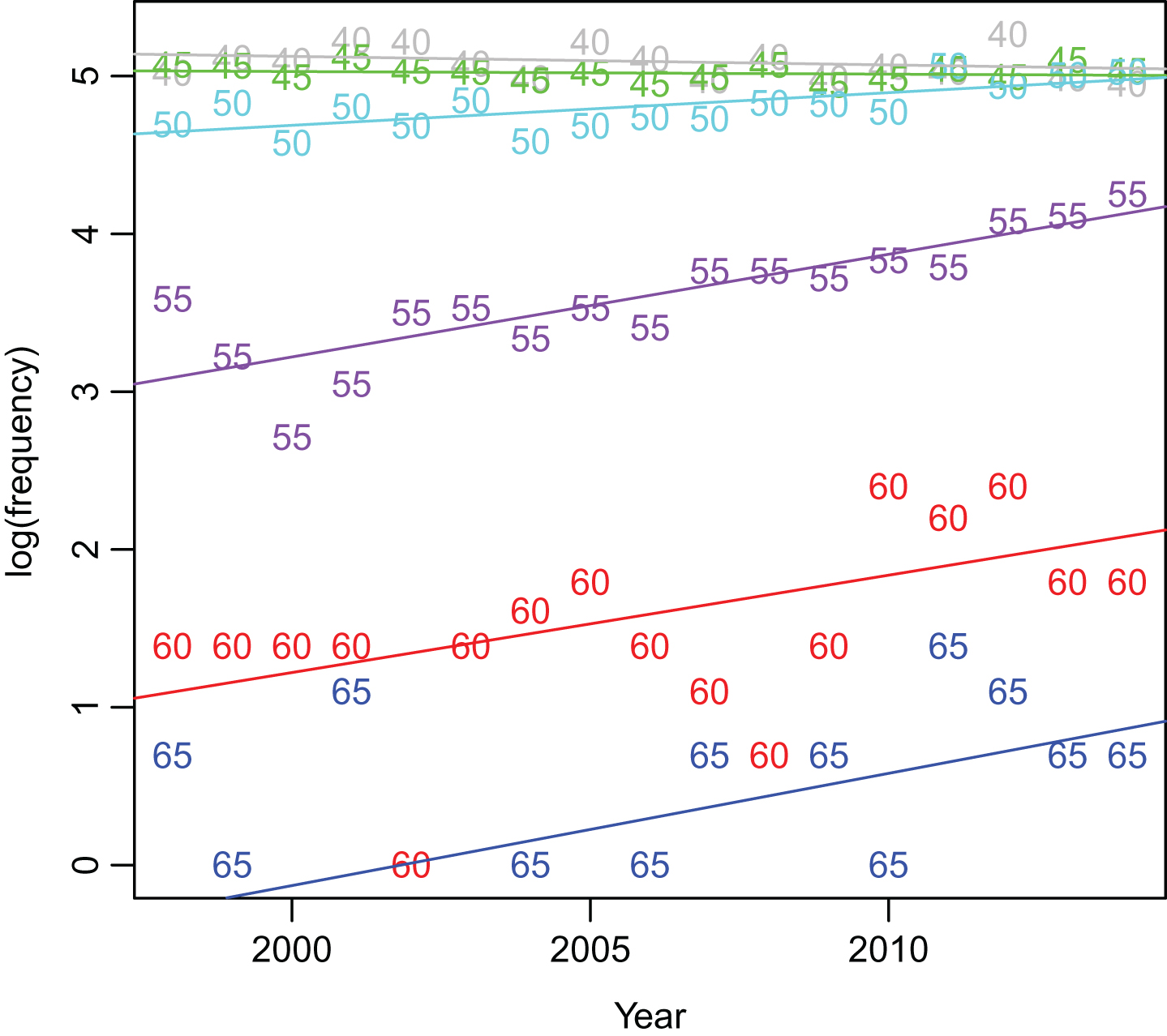
The analyses in this paper cover a wide time span. Kicker ability appears to be changing, especially in the last 10 years, with improving accuracy and experience among kickers (Clark et al., 2013). The frequencies of long field goal attempts are also increasing. Figure 9 shows the log of attempt frequencies against year, with separate plotting characters and colors for each distance, rounded to the nearest five yards. The log-scale is better for visualizing the increase in frequencies. In fact, the log of the frequency of kicks between 53 and 57 yards, denoted in the graph as “55”, and also of kicks between 48 and 52 yards, denoted as “50”, appear to be linearly increasing with season. The figure overlays lines using estimated coefficients from Poisson regressions of frequency on year, separate for each 5-yard distance interval, with the natural log-link function for the generalized linear model. The slopes are significant for distances of 50, 55, and 60 yards.
Fig.9
Log of attempt frequencies over season separated by distances rounded to the nearest five yards starting at 40 yards. Lines are linear regressions of log-transformed attempt frequencies on year.
5Discussion
With the goal of variance-reduction akin to that achieved by Efron and Morris (1975) and Brown (2008) in the prediction of end-of-season batting averages, we presented a flexible framework for the construction of shrinkage estimators of field goal success probabilities. This framework allows for model-based kicker-specific maximum likelihood estimates to be balanced with model-free empirical frequencies aggregated over all kickers. For the model-based estimator, various link functions were assessed using maximum likelihood, Hosmer-Lemeshow statistics and restrictions on data motivated by possible selection bias. The complementary log-log function was selected by all criteria. Findings from several choices for the weight functions of the model-based estimate were presented, including constant, functional, or distribution-based weights, but our investigation was by no means exhaustive. We recommend the midpoint estimator which weights the two components equally on the basis of simplicity and generally good performance as measured by the Hosmer-Lemeshow statistic under cross validation. Interested readers are invited to give other weighting schemes a try. In particular, it seems that low-frequency kickers ought to be estimated using more shrinkage toward the empirical frequency. Since these kickers constitute a comparatively small fraction of the data set, they do not carry much weight as we assess the performance of shrinkage estimators. It is reasonable that in some personnel decisions, they should carry more weight, and a different shrinkage approach and method of assessment may be more appropriate.
Another limitation of the study has to do with failed attempts that are not the fault of the kicker, or perhaps partially the fault of the kicker. If a snap or hold is bad, but an attempt is made and missed, it may appear in a verbal recap, but appears in the play-by-play simply as “no good.” Our model does not account for this type of event. Excluding blocked kicks is also problematic as it is possible that longer attempts may be more likely to be blocked by lesser kickers, so that these failed attempts contain information about kicker ability.
Using the approach of Berry and Berry (1985) to average success probability estimates over the observed distribution of attempt distances, rankings for kickers were provided. Interestingly several current kickers came out on top. In addition to this overall ranking, distance was fixed at several lengths, d = 35, 45 and 55 yards, corresponding roughly to estimated success probabilities for elite (top 20) kickers in the range of 0.9, 0.8, and 0.6 respectively. These estimates are based on a version of the model that expands the degree of polynomial dependence on distance to be quadratic. Presentation of the bestkickers side-by-side enables investigation of kickers who have “big legs,” with a decent shot at long kicks, in comparison to those who are “automatic” at medium distances. An attempt to refine these rankings was made by adding stadium effects, which were found to be highly significant. The estimated marginal (averaged over kickers) means for stadiums with adequate sample sizes were back-transformed to give a ranking of the toughest venues in which to kick.
General managers have made kicker personnel changes with surprising frequency, perhaps overreacting after the sting of a loss which involved a missed field goal. Let us consider the case of Garrett Hartley in more detail. Hartley began his career with the New Orleans Saints in 2008 by making all 13 of his field goal attempts. The following year he made all but two field goal attempts, with the misses coming from 58 and 37 yards. As mentioned in Section 1, in 2010 Hartley missed a 29 yard attempt in overtime in a week 4 loss and the Saints chose to sign John Carney. Carney proceeded to make 5 out of 6 field goals for the two games he replaced Hartley, missing from 29 yards in week 5, the exact same yardage which precipitated Hartley’s demotion. So the following game, Carney was demoted in favor of Hartley and Hartley proceeded to make 16 of the 18 remaining kicks he attempted in the season. The frequency of personnel changes among kickers, averaging more than 3 mid-season cuts per year, is surprising in light of the small number of total kickers over the 16 year period of this study. Though kickers may lose their jobs, many find employment shortly after termination, with a small number moving on through free agency. Whether the high turnover is a result of misunderstanding of the sampling variability inherent in estimating success probabilities from a small number of binary trials, or due to reaction to fan hostility is unclear.
Over the last five years, there has been an increase in the distances at which field goals are attempted, most likely due to increases in kicker abilities. Attempting to model this increase could lead to improvements in the estimation of success probabilities and would be an excellent avenue for further study. Another potentially interesting topic that could be investigated would be the effect of age on elite kickers who have exhibited longevity in the league. Here it is implicitly assumed to be constant, but we may wonder if it is reasonable to expect the same degree of accuracy at all stages of a kicker’s career.
References
1 | Batista J. , (2002) , Pro football; place-kickers at heinz field living in a swirl of trouble, New York Times. |
2 | Berry D.A. and Berry T.D. , (1985) The probability of a field goal: Rating kickers, The American Statistician 39: (2), 152–155. |
3 | Berry S.M. and Wood C. , (2004) , A statistician reads the sports pages: The cold-foot effect, Chance 17: (4), 47–51. |
4 | Bilder C.R. and Loughin T.M. , (1998) , “it’s good!” an analysis of the probability of success for placekicks, Chance 11: (2), 20–30. |
5 | Brown L.D. , (2008) , In-season prediction of batting averages: A field test of empirical bayes and bayes methodologies, The Annals of Applied Statistics, 113–152. |
6 | Carlin B.P. and Louis T.A. , (1997) , Bayes and empirical bayes methods for data analysis, Statistics and Computing 7: (2), 153–154. |
7 | Clark T.K. , Johson A.W. and Stimpson A.J. , (2013) , Going for three: Predicting the likelihood of field goal success with logistic regression, in ‘Sloan Sports Analytics Conference’. |
8 | Dobson A.J. and Barnett A. , (2011) , An introduction to Generalized Linear Models, CRC press. |
9 | Efron B. and Morris C. , (1975) , Data analysis using stein’s estimator and its generalizations, Journal of the American Statistical Association 70: (350), 311–319. |
10 | Gelman A. , Su Y.-S. , Yajima M. , Hill J. , Pittau M.G. , Kerman J. and Zheng T. , (2014) , arm: Data analysis using regression and multilevel/hierarchical models 2010, http://CRAN.R-project.org/package=arm. R package version pp. 1–3. |
11 | Hosmer D.W. and Lemeshow S. , (2004) , Applied Logistic Regression, John Wiley & Sons. |
12 | James W. and Stein C. , (1961) , Estimation with quadratic loss, in Proceedings of the Fourth Berkeley Symposium on Mathematical Statistics and Probability 1: , 361–379. |
13 | McCullagh P. , Nelder J.A. and McCullagh P. , (1989) , Generalized Linear Models 2: , Chapman and Hall London. |
14 | Morris C.N. and Rolph J.E. , (1981) , Introduction to Data Analysis and Statistical Inference, Prentice-Hall Englewood Cliffs Englewood Cliffs, NJ. |
15 | Morrison D.G. and Kalwani M.U. , (1993) , The best nfl field goal kickers: Are they lucky or good? Chance 6: (3), 30–37. |
16 | Pasteur R.D. and Cunningham-Rhoads K. , (2014) , An expectation-based metric for nfl field goal kickers, Journal of Quantitative Analysis in Sports 10: (1), 49–66. |
17 | R Core Team, (2014) , R: A Language and Environment for Statistical Computing, R Foundation for Statistical Computing, Vienna, Austria. http://www.R-project.org/ |
18 | SAS Institute, ((2011) ), SAS/IML 9.3 User’s Guide, SAS Institute. |


