
Position importance in NCAA football
Abstract
To evaluate player and position importance on the BYU football team, we used the coaches’ play-by-play grades of each player as explanatory variables, with the response of expected points gained or lost on each play. Expected points were determined using an analysis of NCAA Football Bowl Subdivision (FBS) teams play-by-play data from 2005–2013 implementing the tiered polychotomous regression model of White and Berry (2002). We used a Bayesian hierarchical linear model with first-level parameters of player and second-level parameters of position to estimate the effect or “impact” each player had on the expected points gained or lost each play. We then used this model to identify the relative importance of each player and each position on the team.
1Introduction
In this paper we propose a novel method of rating players in college football. We will introduce the problem of rating players, the unique dataset obtained to help address the problem, discuss the methods applied to the problem, the results of the methods, and future applications of this research.
1.1Rating players
In college football, coaches are concerned with which players give them the best chance to win. Knowing which positions are “most important” in determining a winning team can help guide recruiting efforts and help in personnel decisions. However, a player being labeled “most important” or “more important" depends on the criteria being used. In many athletic events, a win or loss is of most interest to coaches, players and fans alike. Since scoring points is the main objective, one criteria for players who are important in college football is the ability to create points or diminish the opportunity for the other team to score points. Often, a quarterback (QB) is deemed the “most important” position in football because the QB touches the ball on every offensive possession. Therefore, every good and every bad offensive play has one thing in common, the QB. The QB is given credit for scoring, and the QB is blamed when something goes wrong. In this paper we propose a way to evaluate all players within an offense or defense to determine which position or player actually had the biggest impact on the team’s overall performance in terms of points.
White and Berry (2002) related the QB’s performance in the National Football League (NFL) to the number of points they created. We seek to understand the effect of other positions as well, to bring the inference beyond just the QB. Page et al. (2007) rated every position in the National Basketball Association (NBA) based on the effect they had on the point margin at the end of the game. There is a relatively large literature on skill importance (Florence, et al. 2008; Heiner, et al. 2014; Miskin, et al. 2010; Thomas, et al. 2009) that leads naturally to a consideration of position importance. Conversely, once position importance is explored in football, a natural extension is to consider various football skills and their importance, which would lead to a more efficient partitioning of practice time.
In this paper we develop a methodology that can be used by football teams to rate the relative importance players and positions have on scoring or preventing points in football games. This method can be used as a resource by coaches to better understand how player and position performance relates to points gained or lost in games.
1.2BYU football
To understand the positions and players being rated in our methods, a brief introduction to the Brigham Young University (BYU) football team and their playing style is needed. We focused on the 2015 college football season for our analysis. There are two groups of players in football, the offense and the defense. The offense is responsible for scoring points and consists of 11 positions. The defense is responsible for preventing the opposing team’s offense from scoring points and consists of 11 positions.
On offense BYU typically had five offensive linemen, with a quarterback, one or two running backs, and three or four receivers. Although the offensive line (OL) consisted of players with somewhat different responsibilities (eg. center, who snaps the ball vs. a left tackle who protects the left side of the QB) we will group each of them together in the OL position. The OL’s primary assignment is to prevent defensive players from getting to the QB and to block defenders and clear space for the running back (RB) to make progress up the field. The QB is the position that receives the ball at the start of every play, and his assignment is to hand the ball off to the RB, pass the ball to a receiver, or run the ball himself. As mentioned before, the QB is often viewed as the “most important” position. The RB is either running the ball to make progress towards scoring, or blocking defenders to keep them from tackling another ball carrier. The wide receivers (WR) are the players that line up closest to the sideline on either side. The WR’s primary responsibility is to catch a pass thrown by the QB. The inside wide receivers (IWR) are the receivers who line up closer to the offensive line than the WR’s and had the same job as the WR’s. The IWR’s often made more catches in the middle of the field compared to the WR’s. Tight Ends (TE) were grouped in the IWR for our analysis, but the TE often lined up with the OL and had more OL-type blocking duties than a typical IWR. BYU ran a 3–4 defense in 2015, which means there were three linemen, four linebackers, two corners, and two safeties. Figure 1 shows how the 11 different positions lined up on the field relative to the line of scrimmage. The line of scrimmage is an imaginary line across the field through the ball location that divides the offense from the defense prior to the ball being put in play. The different line positions include the Right End (RE) who lined up on the right of the defensive line, Nose Tackle (Nose) who lined up in the middle of the defensive line, and Left End (LE) who lined up on the left side of the defensive line. These linemen were tasked with tackling or containing the opposing team’s QB, or RB depending on the play the offense was running.
Fig.1
A typical 3–4 defensive formation with position labels. The strong and field side of the field is the left side in this picture, and the weak and boundary side of the field are on the right side.
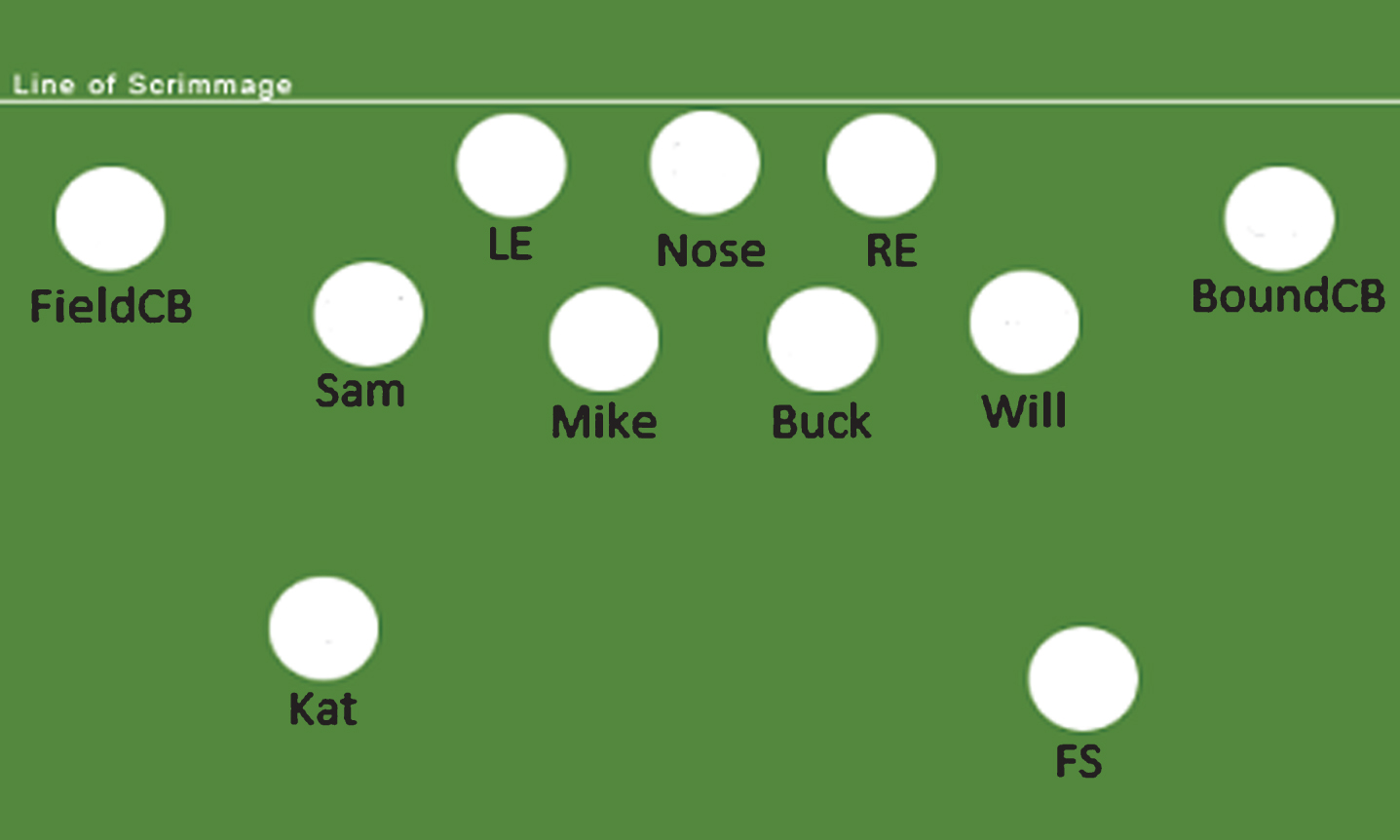
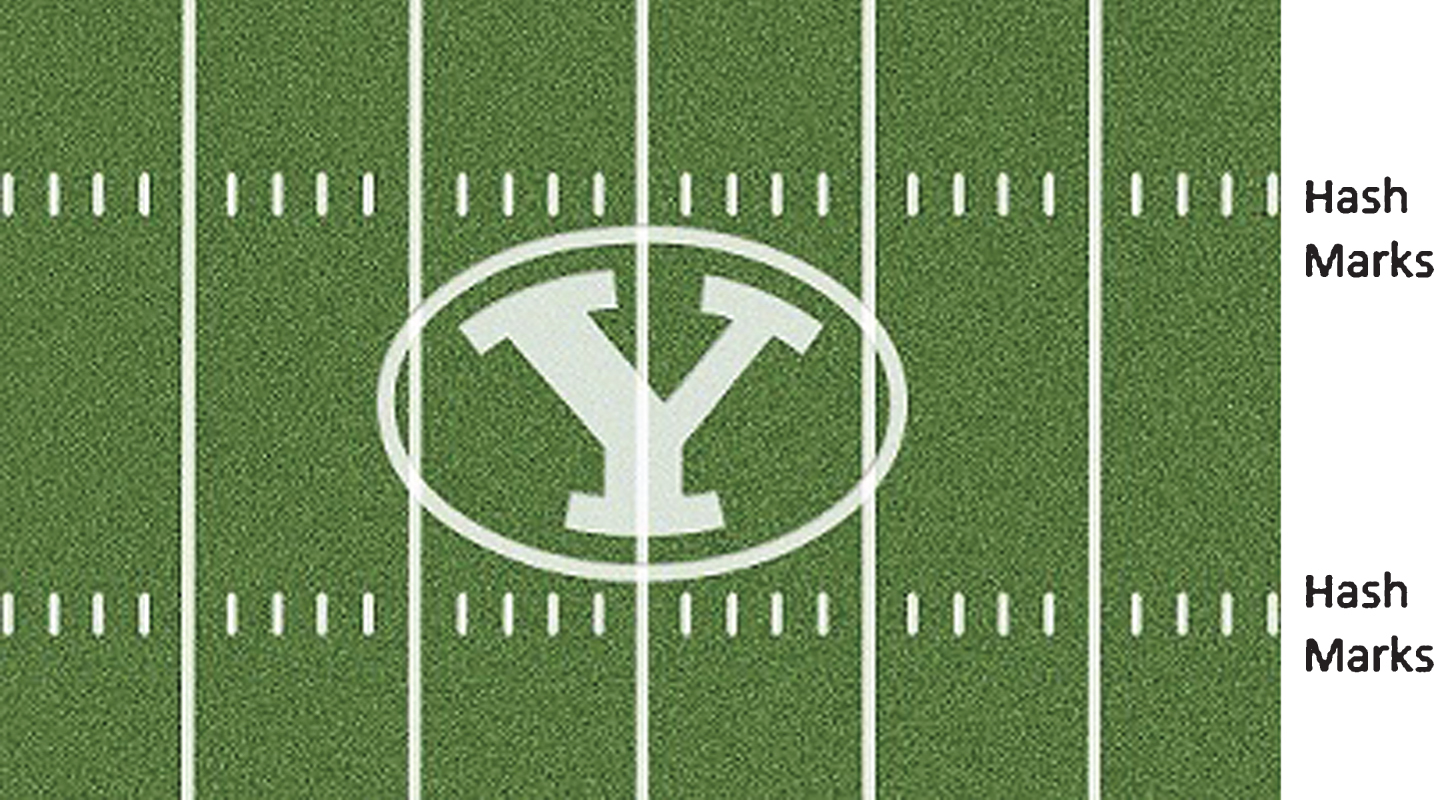
The strong side of the field is the side where more offensive skill positions are lined up, while the weak side is the opposite - the strong and weak side can change from play to play. The four linebackers were separated into outside and inside linebackers. There were two inside linebackers, the Mike - who was responsible for calling the plays for the defense and plays on the strong side of the field, and the Buck - who was responsible for the weak side of the field and acts more as a coverage and containment position. Linebackers communicate to change their alignment on each play if necessary. The outside linebackers consisted of the Sam linebacker - who lined up on the strong side and was usually focused on stopping the run, and the Will linebacker - who lined up on the weak side of the field and helped the secondary (safeties and cornerbacks) contain any receivers, usually opponent’s TE’s or RB’s who went out for a pass. The Will linebacker was often the fastest of the four linebackers because of their coverage duties. The cornerbacks were responsible for covering the receivers and not allowing them to catch the ball, or making a tackle if the receiver did makea catch. The two corners, the field corner (FieldCB) and boundary corner (BoundCB) play on opposite sides of the field. To understand these two sides of the field it is important to understand that the offense would line up at some point between two hash marks that go down the middle of the field, as pictured in Fig. 2. If the offense lined up in the middle of the field, there were equal areas on both the right and left of the offense. However, if the offense lined up closer to or on one of the hash marks, it created a shorter side of the field next to the out of bounds line and a larger side of the field opposite. These two sides are known as the field side (more field to cover) and the boundary or short side. The side of the field corresponding to the position name is where the FieldCB and BoundCB lined up. While both CB positions were responsible for covering WRs the BoundCB had slightly more run responsibility and the FieldCB had slightly more coverage responsibility. If the offense had lined up in the middle of the field, then the FieldCB and BoundCB communicated to determine which side theyplayed on.
Fig.2
An example layout of the hash marks on a football field - if the ball is placed on the top hash mark, the top of the field in this illustration is the boundary side, while the bottom of the field would be called the field side.
The two safeties in BYU’s alignment were the Kat or strong safety, and the free safety (FS). The Kat’s responsibility was to provide pass or run coverage depending on the play. The players who played this position usually had good combinations of cornerback- and linebacker-type skills, because both of those skills were needed. The FS’s responsibility was to cover the pass in whatever area the cornerbacks needed help, and were essentially the cornerbacks safety valve for any extra receivers or missed coverage. The previous paragraphs described the 11 main positions used by BYU, but there were two other positions that were used on occasion. The nickelback (Nickel) was another corner (third corner) that replaced the Kat on plays where the opposing offense lined up extra receivers. The X-Back (XB), sometimes called a dimeback was used when there was a need for two extra cornerback-type players in the game, the Nickel was the first extra cornerback and the XB was the second extra cornerback. The XB often replaced the Sam linebacker when in the game, and was the position that was used least by BYU during the 2015 season.
2Methods
2.1Data
To complete the analysis we propose, the data must contain (1) a way to quantify the team’s production on each play in a game, and (2) a way to rate each player on each play of the game.
To quantify the team’s performance on each play, we first used the model developed by White and Berry (2002) to find the average eventual points or expected points, denoted by E (Pts), a team should score based on the starting position of each play relative to down, distance, and field position. We built an expected points model using data from NCAA Football Bowl Subdivision (FBS) teams from the years 2005–2013. Figure 3 shows E (Pts) for each down given ten yards left to gain for the first down and at each different position on the field.
Fig.3
Expected Points Output, based on a model built on actual points scored in the 2005–2013 FBS division collegiate football games.
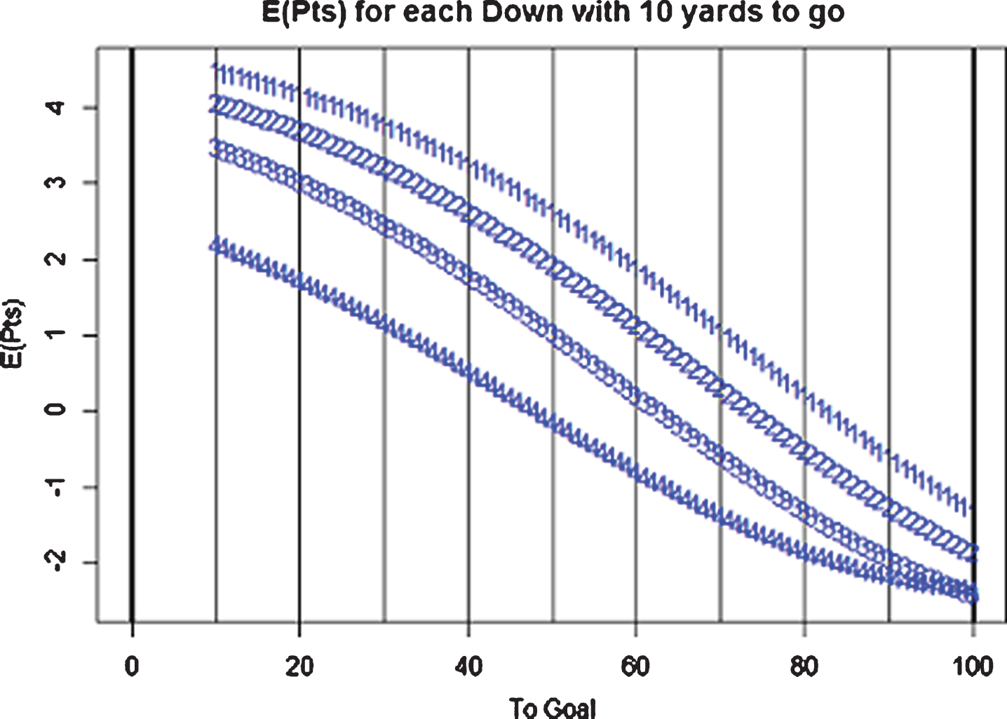
Kovash and Levitt (2009) calculated the change in E (Pts) (ΔE (Pts)) to measure effectiveness of each play. We implemented the same procedure. For example, gaining 15 yards going from 1st and 10 on your own 20 yardline (80 yards to go for a touchdown) (E (Pts) = .22) to 1st and 10 on your own 35 yardline (65 yards to go for a touchdown) (E (Pts) =1.49), would result in ΔE (Pts) =1.27. The ΔE (Pts) value was used as the point value rating for each play in the season.
To rate players and estimate position importance we used data provided by the BYU football coaching staff. During the 2015 season the coaches provided us with a rating for every player on the field for every play (except for any punts, field goals, or victory formation plays). The defensive coaches graded each of their players on a minus or plus scale, with players receiving a minus if they were not assignment-sound on the particular play and a plus otherwise. We converted the minus and plus into zero and one respectively. The offensive coaches graded each of their players on a three-point scale (0, 1, or 2) based on if the player clearly did not do his assignment (0), did an average job executing his assignment (1), or did an exceptional job executing his assignment (2).
We then built a model for each of the different grading systems. The ΔE (Pts) was used as a dependent variable in a model with player ratings as independent variables to asses the contribution of a particular player or position to a team’s overall point production. It is important to note that the ΔE (Pts) in the offensive and defensive models are from the perspective of BYU. So the offensive ΔE (Pts) is calculated just as described above, while the defensive ΔE (Pts) will be positive if the opposing offense had negative ΔE (Pts). This was done so that a more positive coefficient for offense or defense indicates creating E (Pts) for BYU.
2.2Model
Since our response variable, ΔE (Pts), was an expected value, we used a normal likelihood for our data. We used the model written in Equations 1, 2, 3, and 4 as the sampling model. Here i represents the play number within the game or season. One of the benefits of this model comes from the ability to use it to analyze any subset of plays one might be interested in - whether it is a group of plays, one single game, a combination of games, or an entire season. We used this model formulation to investigate each individual BYU game as well as the entire season in several different model runs. For the offense, oi represents the offensive players on the field for the ith play, while j represents a player who played in the subset of plays being modeled. k is the indicator for offense (denoted by o) or defense (denoted by d). For the defense, di represents the players in each defensive position on play i. Within our data, the defense had 13 different positions that were rotated depending on the formation. This meant two of the defensive positions were empty each play. The missing positions were modeled by a specific βjd in this case to help measure formation effectiveness and the effect of a position not being in the game. There were also players who played multiple positions on defense, so they had separate βjd’s for the different positions they played. The xij are the coaches’ grade of the jth player on the ith play, xij ∈ {0, 1, 2} for the offense and xij ∈ {0, 1} for the defense. While the sampling model enabled us to model player performance through the βj’s, we also wanted to model the position performance. To do this, a Bayesian hierarchical model was implemented. The priors for the parameters in the sampling model are outlined in Equations 5–9. Equations 5–7 show the assumed prior distributions for the model parameters. Equations 8 and 9 are the assumed hyperprior distributions for the hierarchical parameters. The θz’s are the parameters that model average position performance, and the ξz’s model position performance variability. The z corresponds to the position the player in play j is playing.
1 Offense: z∈{QB, RB, WR, IWR, OL}
2 Defense: z∈{RE, Nose, LE, Mike, Buck, Sam, Will, FieldCB, BoundCB, Kat, FS, Nickel, XB}
(1)
(2)
(3)
(4)
(5)
(6)
(7)
(8)
(9)
2.2.1Choices
We used gamma priors for the variances and the parameters were chosen to give a mean of two and variance of one. The E (Pts) only range from around negative two to positive five, so a variance in ΔE (Pts) around two is reasonable. This parameterization also preserved the parameter space for
2.2.2Estimating the posterior
To estimate the posterior distribution of each of the parameters for the offense and defense we used Markov chain Monte Carlo methods (Gelman, et al., 2014). We used JAGS (Plummer, 2003) as our modeling software.
3Results
Since our player ratings were obtained using proprietary data, we do not include estimates for individual players. We do, however, include each of the overall position estimates. Tables 1 and 2 list mean, standard deviation and the importance score used by Miskin, et al. (2010) (
Table 1
Offense posterior point estimates for positions in full season model
| θz | E (θz) | sd (θz) | IS |
| θIWR | 0.05 | 0.79 | 0.06 |
| θOL | 0.06 | 0.66 | 0.09 |
| θWR | 0.11 | 1.01 | 0.11 |
| θRB | 0.15 | 1.05 | 0.14 |
| θQB | 0.26 | 1.34 | 0.19 |
Table 2
Defense posterior point estimates for positions in full season model
| θz | E (θz) | sd (θz) | IS |
| θLE | –0.10 | 0.22 | –0.45 |
| θNose | –0.22 | 0.50 | –0.44 |
| θXB | –0.15 | 0.39 | –0.39 |
| θSam | –0.10 | 0.52 | –0.19 |
| θWill | –0.09 | 0.53 | 0.17 |
| θFieldCB | 0.20 | 0.71 | 0.28 |
| θBuck | 0.10 | 0.26 | 0.38 |
| θFS | 0.27 | 0.52 | 0.52 |
| θKat | 0.21 | 0.40 | 0.53 |
| θNickel | 0.16 | 0.20 | 0.80 |
| θRE | 0.51 | 0.32 | 1.61 |
| θMike | 0.34 | 0.17 | 1.96 |
| θBoundCB | 0.54 | 0.20 | 2.70 |
Figures 4–7 show the density estimates for the position posteriors for three different models, the models executed on plays in the BYU vs Boise State game (BYU won 35–24), the BYU vs Missouri (Mizzou) game (Mizzou won 20–16) and the entirety of games graded by the BYU coaches during the season. We did not receive the Nebraska, UCLA, Wagner, Utah State and Utah game grades for the offense, and the Wagner, and Utah game grades for thedefense.
Fig.4
Offense posterior distributions for θ by position.
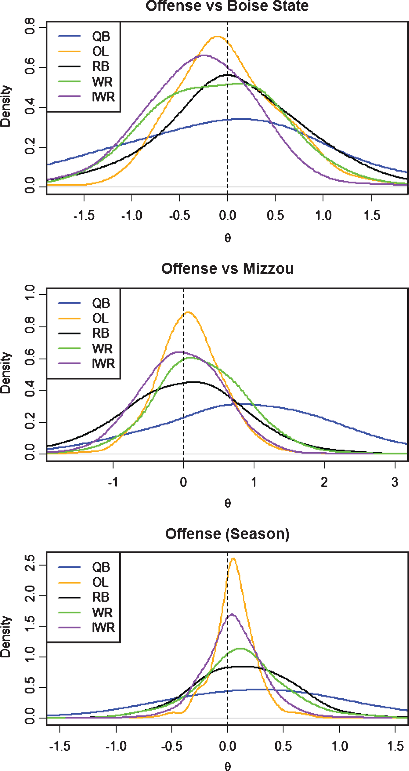
Fig.5
Defensive Line posterior distributions for θ by position.
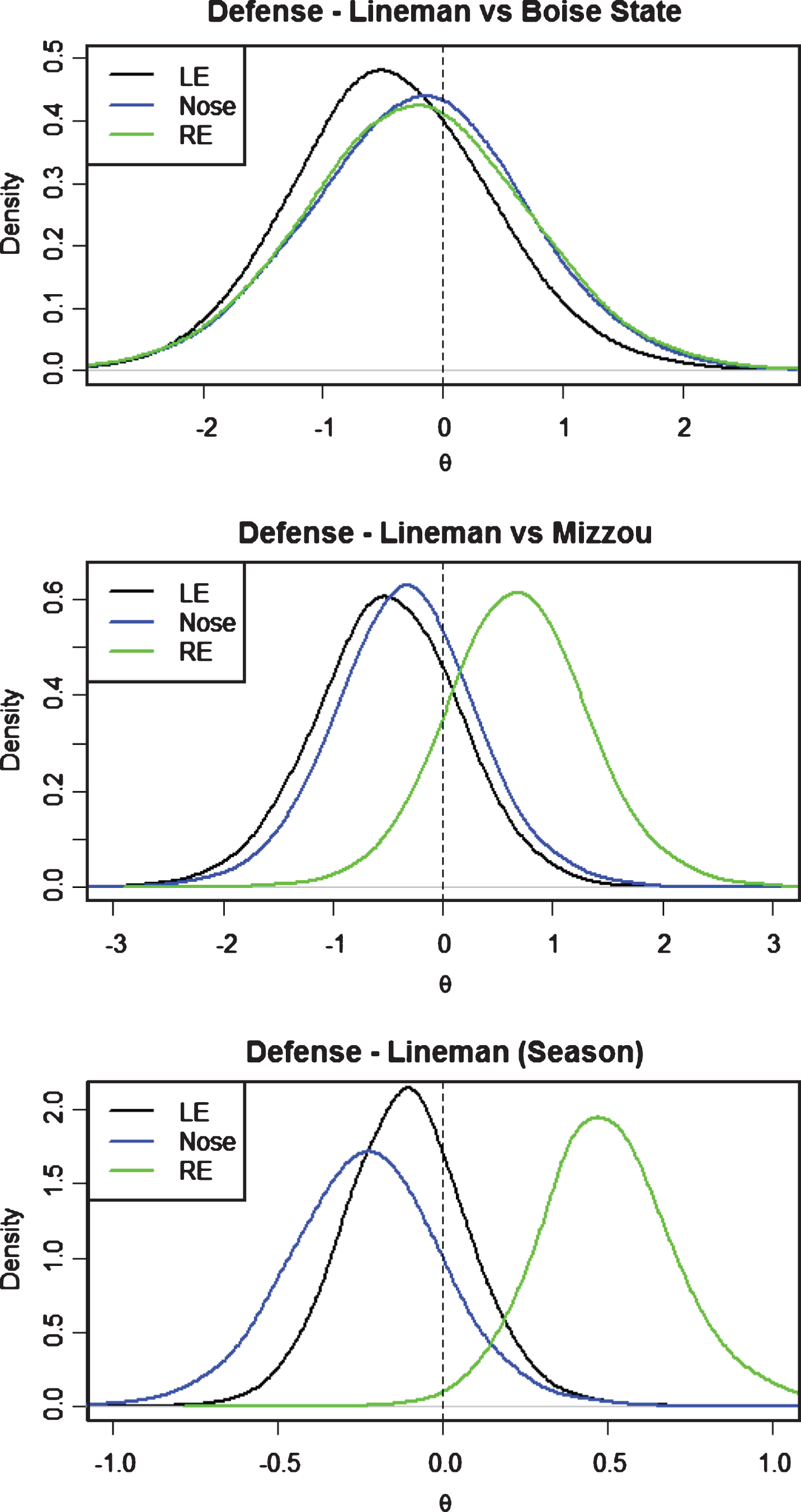
Fig.6
Defensive LB’s posterior distributions for θ by position.

Fig.7
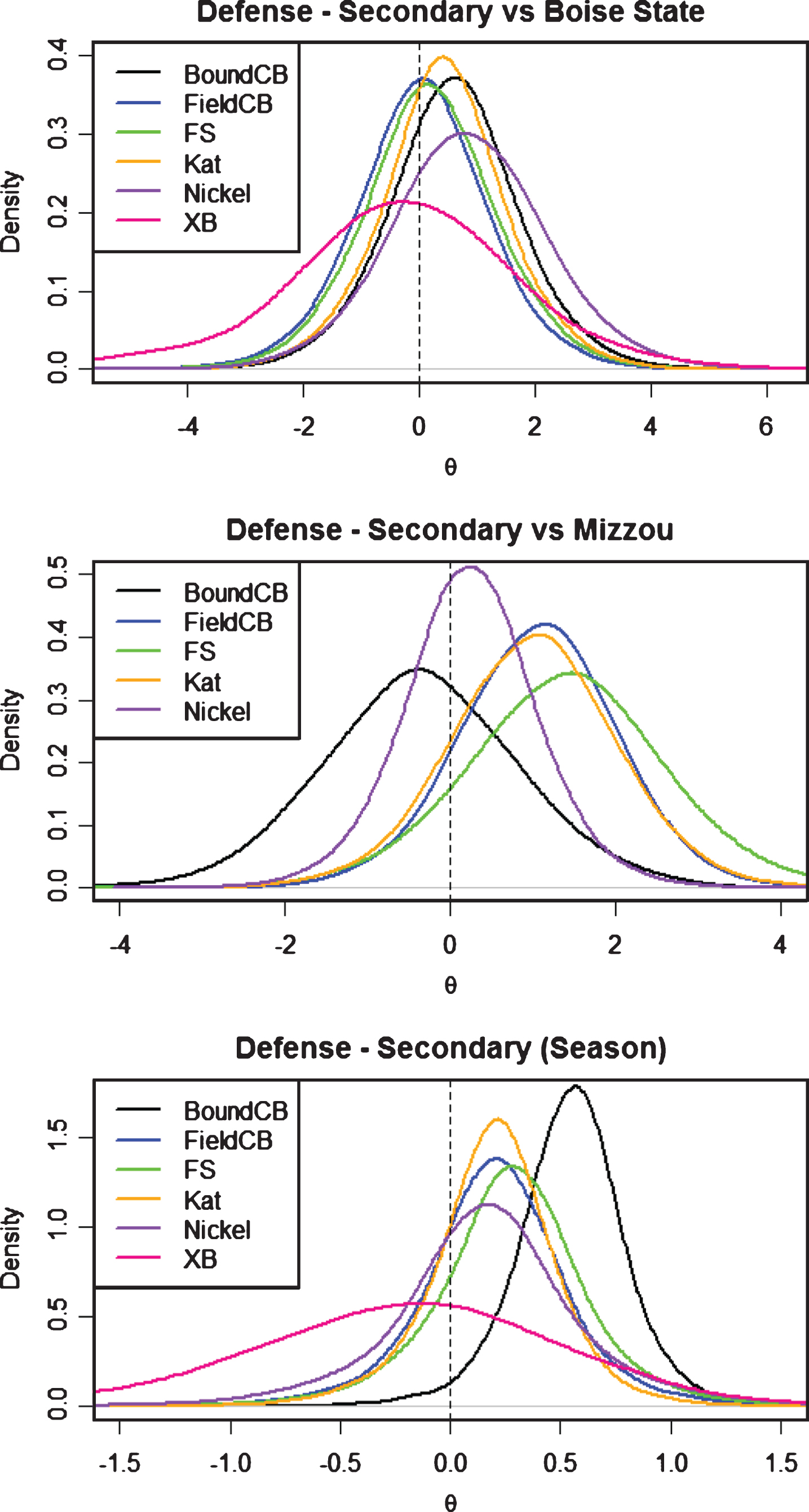
Defensive Secondary posterior distributions for θ byposition.
When looking at the posterior density estimates of theta for the positions (θz), it is important to keep in mind that this is the effect a position has on ΔE (Pts) when they are judged by the coaches to have executed their specific positional assignment.
3.1Offense
Our result matched the intuition of other experts in that the QB was the “most important” position for the offense. Table 1 shows that the QB had the highest importance score. When the QB executed his assignment, it had the largest positive effect on ΔE (Pts). However, the variability of that effect was also quite large. The large variability associated with the QB position may be explained by the QB’s dependence on other positions. For example, a perfect pass (rated highly by the coach) is dropped by the receiver, resulting in a negative change in E (Pts). The RB and WR were the next “most important” positions for the offense in terms of importancescore.
Figure 4 shows the posterior density estimates for each position. In the season model the QB continues to show the pattern of added variability, which we attributed to the reliance of the position on other positions as well as the appearance of two different QB’s with varying levels of skill within the season’s analysis. It also appeared that the skill positions (QB, WR, RB) had the largest effect on ΔE (Pts). These results were generally expected as the skill positions were most widely regarded as the play-making positions among those associated with BYU football during the 2015 season. The high variability of these skill position effects is important to keep in mind when trying to understand the consistency of the position effects. For a coach who obtained this information, it would be important to then explore the player effects to understand which players inside each of the positions were most consistent and had more positive effects.
In Table 3 we see the game by game change of β0o. The β0o value can be interpreted as the expected ΔE (Pts) if every position did not complete their assignment. The average value of β0o for the Boise State game was 0.56 compared to -2.06 for the Mizzou game. This indicated that the team was performing at a negative ΔE (Pts) rate most of the game, and the only position that created better ΔE (Pts) plays from executing their assignment was the QB.
Table 3
Offense posterior β0o estimates for each game analyzed in 2015
| Opponent | E (β0o) | sd (β0o) |
| Boise State | 0.56 | 1.11 |
| Michigan | –1.8 | 1.36 |
| Connecticut | –2.18 | 0.57 |
| ECU | –1.55 | 0.67 |
| Cincinatti | –2.83 | 0.87 |
| SJSU | 0.17 | 0.81 |
| Mizzou | –2.06 | 0.71 |
| Fresno State | –0.64 | 0.87 |
| Season | –1.39 | 0.24 |
3.2Defense
The defensive results are formatted to be consistent with the offensive results, but it is important to remember that the defensive grades were on a two-point scale instead of the three-point scale used by the offense. There are also a larger number of positions on the defense compared to the offense. Because of this we will rely more on the importance scores to find differences in position importance.
For the defense, we anticipated that the Mike would be the “most important” position because of his play calling responsibilities. Table 2 indicates that the average impact the Mike had from executing his assignment was in the top-tier of the defensive positions, but not the largest. From the importance score estimates it is clear that the BoundCB, Mike and RE were the top three most important defensive positions in that order. The importance scores also make it clear that the LE, Nose, XB, and Sam positions are less important. Having a negative estimate indicates that the defense as a whole has a more negative ΔE (Pts) when the positions execute their assignment. Figures 5, 6, and 7 show the posterior position density estimates for the models run on the same games as in the offense discussion as well as the full season model.
In each of the position groups, we note that the positions were more grouped together in the win (vs Boise State) compared to the loss (vs Mizzou). This shows a less consistent across-defense performance in the loss when compared to the win. We again saw the difference in the β0d for the two games in Table 4. The win had a β0d of –1.86 while the loss had a β0d of –2.65. This difference was not quite as big of a difference as the offense comparison, but still explained a portion of the differing performances. Another thing to keep in mind is that both of these games were very close and could have gone either way toward the end, so the win-loss result cannot be the entire issue. However, the results of the position estimates did indicate that the Boise State game was a more consistent team performance.
Table 4
Defense posterior β0d estimates for each game analyzed in 2015
| Opponent | E (β0d) | sd (β0d) |
| Nebraska | –2.00 | 1.51 |
| Boise State | –1.86 | 2.04 |
| UCLA | –1.74 | 3.74 |
| Michigan | –2.16 | 1.8 |
| Connecticut | –0.66 | 3.7 |
| ECU | –1.38 | 2.86 |
| Cincinatti | –2.13 | 1.87 |
| SJSU | 0.55 | 3.66 |
| Mizzou | –2.65 | 3.45 |
| Fresno State | –2.86 | 4.11 |
| Utah State | –0.39 | 3.05 |
| Season | –1.92 | 0.22 |
Among position groups, there were some clear findings as well. For defensive linemen, it was very evident that the RE position had the largest effect on ΔE (Pts) - indicating that during the 2015 season, the RE was the “most important” position on the defensive line (Fig. 5). This result may also indicate that the LT is more important than the RT on the offensive line, although we could not see this as the OL positions were not discriminated at this level. The linebacker group was more clustered, but it did show that the Mike was slightly more important than the other linebacker positions (Fig. 6). We believed this showed the importance of the Mike position in calling the play, as often the Mike’s grade reflected the way the play was communicated to the rest of the defense. The play calling was important because it gave each of the other positions the assignment they needed to execute for each play. In the secondary group, the BoundCB was the “most important” position - this indicated that the BoundCB needed to execute his assignment to prevent the opposing offense from having more positive ΔE (Pts) plays. This specific rating may be reflective of the big plays the BoundCB can be susceptible to giving up. BYU football had historically struggled with cornerbacks, and this analysis seemed to point to the need of having a BoundCB that can execute each and every play.
4Conclusion
Although we understand that many of the results are open to interpretation, we do feel that providing quantitative evidence to facilitate discussion among coaches in determining position and player impact would help any football team improve their overall performance. In general applications, the player rating system yields estimates for every position, thus allowing evaluation of all players. Our analysis was hampered by two issues. (1) Not all games were graded, we are missing the Nebraska, UCLA, Wagner, Utah State and Utah games for the offense, and the Wagner, and Utah games for the defense. And (2) the grades supplied by the position coaches were not well calibrated. For the methodology we implemented here to be most precise, the coaches supplying the grades need to be working closely together to provide consistent grades. Nonetheless, we believe this methodology has potential to yield useful information for football teams relative to both individual player and position importance.
We find specific value in using these ratings to focus recruiting efforts in the more important positions. The model could also be very useful for coaches when they have two players at a position that they feel are equal - as it can provide quantitative differences between the two players in question. We hope to apply this to different offensive units, formations and skills in future work. Skills would be of particular interest in the linebacker and secondary positions - where the analysis could help determine if tackling or coverage skills were more important.
Acknowledgments
Salary support for the first author was provided by the Athletic Department at Brigham Young University.
References
[1] | Florence L.B. , Fellingham G.W. , Vehrs P.R. and Mortensen N. , (2008) , Skill evaluation in women’s volleyball, The Journal of Quantitative Anlysis in Sports 4: (2), Article 14. |
[2] | Gelman A. , Carlin J.B. , Stern H.S. , Dusnon D.B. , Vehtari A. and Rubin D.B. , (2014) , Bayesian Data Analysis, 3 edition. |
[3] | Heiner M. , Fellingham G.W. and Thomas C. , (2014) , Skill importance in women’s soccer, Journal of Quantitative Analysis in Sports 10: (2), 287–302, ISSN (Online) 1559-0410, ISSN (Print) 2194-6388, DOI: 10.1515/jqas-2013-0119 |
[4] | Kovash K. and Levitt S.D. , (2009) , Professionals do not play minimax: Evidence from major league baseball and the national football league, Working Paper 15347, National Bureau of Economic Research, URL http://www.nber.org/papers/w15347. |
[5] | Miskin M. , Fellingham G.W. and Florence L.B. , (2010) , Skill importance in women’s volleyball, The Journal of Quantitative Analysis in Sports 6: (2), Article 5. |
[6] | Page G.L. , Fellingham G.W. and Reese C.S. , (2007) , Using box-scores to determine a position’s contribution to winning basketball games, The Journal of Quantitative Analysis in Sports, 3: (4), Article 1. |
[7] | Plummer M. , (2003) , Jags: A program for analysis of bayesian graphical models using gibbs sampling, Proceedings of the 3rd International Workshop on Distributed Statistical Computing (DSC 2003). |
[8] | Thomas C. , Vehrs P.R. and Fellingham G.W. , (2009) , Development of a notational analysis system for selected soccer skills of a women’s college team, Measurement in Physical Education and Exercise Science 13: (2):108–121. |
[9] | White C. and Berry S. , (2002) . Tiered polychotomous regression: Ranking NFL quarterbacks, The American Statistician 56: , 1021. |

