
A scalable framework for NBA player and team comparisons using player tracking data
Abstract
Player tracking data provides a platform for the creation of new basketball statistics that can dramatically improve the ability to evaluate and compare player performance. However, the increasing size of this new data source presents challenges in how to efficiently analyze the data and interpret findings. A scalable analytical framework is needed that can effectively reduce the dimensionality of the data while retaining the ability to compare player performance.
In this paper, Principal Component Analysis (PCA) is used to identify four components accounting for 68% of the variation in player tracking data from the 2013-2014 regular season. The most influential statistics on these new dimensions are used to construct intuitive, practical interpretations. In this high variance, low dimensional space, comparisons across any or all of the principal components are possible to evaluate characteristics that make players and teams similar or unique. A simple measure of similarity between player or team statistical profiles based on the four principal components is also constructed. The Statistical Diversity Index (SDI) allows for quick and intuitive comparisons using the entirety of the player tracking data. As new statistics emerge, this framework is scalable as it can incorporate existing and new data sources by reconstructing principal component dimensions and SDI for improved comparisons.
Using principal component scores and SDI, several use cases are presented for improved personnel management. Team principal component scores are used to quickly profile and evaluate team performance, more specifically how New York’s lack of ball movement negatively impacted success despite high average scoring efficiency as a team. SDI is used to identify players across the NBA with the most similar statistical performances to specific players. All-Star Tony Parker and shooting specialist Anthony Morrow are used as two examples and presented with in-depth comparisons to similar players using principal component scores and player tracking statistics. This approach can be used in salary negotiations, free agency acquisitions and trades, role player replacement, and more.
1Introduction
The National Basketball Association (NBA) launched a public database in September 2013 containing new statistics captured by STATS LLC through their innovative sportVU player tracking camera systems (NBA partners with Stats LLC for tracking technology, 2013). The cameras capture and record the location of players on the court as well as the location of the ball, and the data are used to derive statistics that expand greatly upon traditional statistics available for analysis of basketball performance. We can now break down shot attempts and points by shot selection (e.g. driving shots, catch and shoot shots, pull up shots), assess rebounding ability for contested and uncontested boards, and look at new statistics like average speed and distance and opponent field goal percentage at the rim. The availability of such data enables fans and analysts to dig into the data and uncover insights previously not possible due to the limited nature of the data at hand.
For example, techniques to uncover different ‘positions’ based on grouping statistical profiles have become increasingly popular. It reflects the mindset of current NBA coaches and general managers who are very much aware of the different types of players beyond the five traditional roles. However, a recent proposal (Alagappan, 2012) has received criticism for its unintuitive groupings and inability to separate out the impact of player talent (Haglund, 2012). The NBA player tracking data has the ability to differentiate player performance across more dimensions than before (e.g. shot selection, possession time, physical activity, etc.) which can provide better ways to evaluate the uniqueness and similarities across NBA player abilities and playing styles. Another example is in the development of offensive and defensive ratings. Current methods require an estimation of possessions and other statistics to produce ratings (Oliver et al., 2007). With the ability to track players’ time of possession and proximity to players in possession of the ball through player tracking, we can develop more accurate representations of possessions and better player offensive and defensive efficiency metrics.
However, the high dimensionality of this new data source poses major challenges as it demands more computational resources and reduces the ability to easily analyze and interpret findings. We must find a way to reduce the dimensionality of the data set while retaining the ability to compare player performance. One method that is particularly well-suited for this application is Principal Component Analysis (PCA) which identifies the dimensions of the data containing the maximum variance in the data set. This article applies PCA to the NBA player tracking data to discover four principal components that account for 68% of the variability in the data for the 2013-2014 regular season. These components are explored in detail by examining the player tracking statistics that influence them the most and where players and teams fall along these new dimensions.
Additionally, a simple measure of similarity in statistical profiles between players and teams based on the principal components is proposed. The Statistical Diversity Index (SDI) can be calculated for any pairwise player combination and provides a fast and intuitive method for finding players with similar statistical performances along any or all of the principal component dimensions. This approach is also advantageous from the standpoint of scalability. The possibilities to derive new statistics from the player tracking data are endless, so as new statistics emerge, this approach can again be applied using the new and existing data to reconstruct the principal components and SDI for improved player evaluation and comparisons.
Numerous applications in personnel management exist for the use of SDI and principal component scores in evaluating and comparing player and team statistical performances. Two specific case studies are presented to show how these tools can be used to quickly identify players with similar statistical profiles to a certain player of interest for the purpose of identifying less expensive, similarly skilled players or finding suitable replacement options for a key role player within the organization.
This article is organized as follows. Section 2 describes the player tracking data and data processing. Section 3 provides the analysis and interpretations for the four principal components in detail, showing how players and teams can be compared across these new dimensions. Section 4 introduces the calculation for SDI and two case studies where principal component scores and SDI are used to find players with similar statistical profiles to All-Star Tony Parker and role player Anthony Morrow for personnel management purposes. 5 conclusion concludes the article with final remarks.
2NBA player tracking data
2.1Data description
Currently, there are over 90 new player tracking statistics, and data for all 482 NBA players from the 2013-2014 regular season are available. Separate records exist for players who played for different teams throughout the season, including a record for overall performance across all teams. Brief descriptions of the newly available statistics adapted from the NBA player tracking statistics website (Player Tracking, 2016) are provided for reference and will be helpful in better understanding the analysis going forward.
Shooting
Traditional shooting statistics are now available for different shot types:
• Pull up shots - shots taken 10 feet away from the basket where player takes 1 or more dribbles prior to shooting
• Driving shots - shots taken where player starts 20 or more feet away from the basket and dribbles less than 10 feet away from the basket prior to shooting
• Catch and shoot shots - shots taken at least 10 feet away from the basket where player possessed the ball for less than 2 seconds and took no dribbles prior to shooting
Assists
New assist categories are available that enhance understanding of offensive contribution:
• Assist opportunities - passes by a player to another player who attempts a shot and if made would be an assist
• Secondary assists - passes by a player to another player who receives an assist
• Free throw assists - passes by a player to another player who was fouled, missed the shot if shooting, and made at least one free throw
• Points created by assists - points created by a player through his assists
Touches
Location of possessions provides insight into style of play and scoring efficiency:
• Front court touches - touches on his team’s offensive half of the court
• Close touches - touches that originate within 12 feet of the basket excluding drives
• Elbow touches - touches that originate within 5 feet of the edge of the lane and the free throw line inside the 3-point line
• Points per touch - points scored by a player per touch
Rebounding
New rebounding statistics incorporate location and proximity of opponents:
• Contested rebound - rebounds where an opponent is within 3.5 feet of the rebound
• Rebounding opportunity - when a player is within 3.5 feet of a rebound
• Rebounding percentage - rebounds over rebounding opportunities
Rim Protection
When a player is within 5 feet of the basket and within 5 feet of the offensive shooter, opponents’ shooting statistics are available to measure how well a player can protect the basket.
Speed and Distance
Players’ average speeds and distances traveled per game are also captured and broken out by offensive and defensive plays.
2.2Data processing
Only players who played at least half the 2013-2014 regular season, 41 games, are included in this analysis. This restriction is made to reduce the influence of player statistics derived from only a few games played. Also fields containing season total statistics and per game statistics are dropped from the analysis since they could be influenced by number of games and minutes played throughout the season. Instead, per 48 minutes, per touch, and per shot statistics are used. The final data set contains 360 player records each containing 66 different player tracking statistics.
3Principal component analysis
With numerous player tracking statistics already available and the potential to develop infinitely many more, it is difficult to extract meaningful and intuitive insights on player comparisons. Now that the data are available for more granular and detailed comparisons, a methodology is needed that can analyze the entirety of the data set to extract a handful of dimensions for comparisons. These dimensions should be constructed in a way that ensures optimality in differentiating players (i.e. dimensions should retain the maximum amount of player separability possible from the original data) and can be understood in terms of the original statistics.
Principal Component Analysis (PCA), developed by Karl Pearson (Pearson, 1901) and later by Hotelling (Hotelling, 1933), is a particularly well-suited statistical tool that can accomplish this task through identifying uncorrelated linear combinations of player tracking statistics that contain maximum variance. Interested readers can find a brief technical introduction to PCA in Appendix A. Components of high variance help us better differentiate player performance in these directions in hopes that the majority of the variance will be contained in a small subset of components. This simple and intuitive approach to dimension reduction provides a platform for player comparisons across dimensions that best separate players by statistical performance and can be implemented withoutexpensive proprietary solutions, providing more visibility into how the method works at little to no additional cost.
3.1Dimension reduction
PCA is sensitive to different variable scalings in the original data set such that variables with larger variances may dominate the principal components if not adjusted. To set every statistic on equal footing, all statistics are standardized with mean 0 and variance 1 prior to conducting the analysis.
PCA is most useful when the majority of the total variance across variables are captured by only a few of the principal components, thus the dimension reduction. If this is the case for the NBA player tracking data set, it means that we are able to retain the ability to differentiate player performance without having to operate in such a high dimensional space. Figure 1 scree shows the variance captured by each principal component. Note the variance captured in the first principal component is very high and decreases drastically through the first four components. After that, the change in variance is relatively flat, forming an elbow shape in the plot. This means that the variances captured by the fifth component onward are very similar and much smaller than the first four components. Moreover, the first four components capture 68% of the variance across the original variables, so we utilize these four components going forward to analyze and compare player performance and playing styles.
3.2Principal components
Each principal component (PC) is a linear combination of the original variables in the dataset. There is a vector for each principal component containing the coefficients associated with each of the variables in the original data set and are called loading vectors. These describe the influence of each variable for each principal component and are used to interpret these new dimensions in terms of the original variables. Figure 2 pcload plots the categorized loading coefficients for the four principal components and is explored in detail in the following sections. Variables can have a positive or negative contribution to the principal component. While the sign is arbitrary, understanding which variables contribute positively or negatively can help with interpreting the principal components. The most important statistics for each component are presented in the following sections, but tables containing all loading coefficients for variables contributing significantly to the principal components are also available in Appendix B for more details.
Each player can then be given a set of PC scores by multiplying the standardized statistics by their corresponding loading coefficients and then taking a sum (see Appendix A for details). Figure 3 contains plots of the PC scores for all players with a select few noted for illustration. Using the loading and score plots here, we can begin to understand and interpret what these new dimensions are capturing and use them for player comparisons.
3.2.1PC 1: Inside vs. Outside
The first principal component accounts for the most variation, 42% of the total variance. Table 1 lists statistics with highly positive and negative loadings for PC 1. Refer to Figure 2 for categorized PC 1 loadings for all statistics. These are used to better understand the meaning of the scores along this dimension. Players with positive scores for PC 1 are able to secure rebounds of all kinds and are responsible for defending the rim and close shots. Notable examples are Andre Drummond, DeAndre Jordan, and Omer Asik. Players with negative scores for PC 1 drive the basketball to the hoop and take pull up and catch and shoot shots often, which implies they tend to be outside players. These players also tend to possess the ball more often and generate additional offense through assists. Examples here are Stephen Curry, Tony Parker, and Chris Paul.
3.2.2PC 2: Assist and Drive vs. Catch and Shoot
PC 2 accounts for another 12% of the total variance and Table 2 lists statistics with highly positive and negative loadings. Also refer to Figure 2 for categorized PC 2 loading coefficients. Players with positive PC 2 scores generate offense mainly through assists and driving shots. These players tend to possess the ball often and either kick the ball to teammates for shot attempts or drive the ball to the basket. Many point guards fall into this category with examples like Ricky Rubio, Tony Parker, and Chris Paul. Players with negative PC 2 scores provide offense primarily through catch and shoot shots and are very efficient scorers, especially from behind the 3-point arc. Primary examples are Klay Thompson, Kyle Korver, and Anthony Morrow.
3.2.3PC 3: Scoring and Rebounding Efficiency vs. Speed
Table 3 lists statistics with highly positive and negative loadings for PC 3 which explains 9% of the total variance. Also refer to Figure 2 for categorized PC 3 loading coefficients. Players with positive PC 3 scores are extremely quick on both sides of the ball and cover a lot of ground while on the court. Some examples are Ish Smith, Shane Larkin, and Dennis Schroder. Players with negative PC 3 scores are largely responsible for scoring when on the court and provide a significant amount of offensive production per 48 minutes. Scoring and rebounding efficiency characterize many of the superstars in the NBA with players like Kevin Durant, Carmelo Anthony, and LeBron James touting highly negative PC 3 scores.
3.2.4PC 4: Catch and Pass/Shoot vs. Slash
Table 4 lists statistics with highly positive and negative loadings for PC 4 which accounts for another 4% of the total variance. Also refer to Figure 2 for categorized loading coefficients for PC 4. This component is characterized by players’ tendencies when they receive possession of the ball. Players with positive PC 4 scores tend to pass or convert catch and shoot shots when the ball goes their way (e.g. Kevin Love, Spencer Hawes, and Patty Mills) while players with negative PC 4 scores tend to drive the ball and score efficiently when they get touches (e.g. Tyreke Evans, Rodney Stuckey, and Tony Wroten).
3.3Team PC Scores
Not only can we characterize players by principal components, but teams can also be profiled along these new dimensions as well. There are numerous ways to aggregate the player PC scores to form a team-level score, but here a simple weighted average is used. The kth team PC score, tk(team), can be found by taking an average of the kth PC scores across the n players weighted by the minutes played throughout the season, mi, i = 1, …, n.
(1)
Figure 4 shows the distribution of all NBA teams across these dimensions as well as their corresponding 2013-2014 regular season winning percentage. This view is useful in seeing the differences and similarities in team playing styles and how they impact success.
For example, the New York Knicks had an extremely negative PC 2 score. Further investigation shows it is partially the result of catch and shoot offense from J.R. Smith, Andrea Bargnani, and Tim Hardaway Jr. who were all in the top 50 in catch and shoot points per 48 minutes. However, another major factor is that 8 of the 12 New York players were below average in passes per 48 minutes (average was 58 passes per 48 minutes) which is indicative of poor ball movement. All-Star Carmelo Anthony is in this group and has long been labeled a “ball hog” (Naessens, 2014) which is supported by his below average passing and above average number of touches and scoring. In fact, Anthony’s top 10 performance in points per 48 minutes, points per touch, and rebounding efficiency helped earn his team the most negative PC 3 team average score. Note that team average PC 3 score is negatively correlated with winning percentage, yet the Knicks won only 37 games and failed to make the playoffs.
To better understand how these team average PC scores impact winning, Table 5 contains the results from a multiple linear regression analysis on winning percentage. Note that negative PC 3 scores are highly correlated with winning while positive PC 2 and PC 4 scores are also highly correlated with winning. Negative PC 3 scores are associated with high average scoring and rebounding efficiency. Referring back to Tables 2 and 4, passes, touches, and assists contribute positively to PC 2 and PC 4 scores. Regarding New York’s lackluster season, it seems that Anthony’s great offensive production was not enough to offset the negative impact of extremely poor passing and ball movement.
These results are better illustrated in Figure 5 where the regression-weighted sum of PC 2 and PC 4 scores (0.17*[PC 2 Score] + 0.09*[PC 4 Score]) determine the size of the points. Low average PC 3 scores (i.e. high average scoring and rebounding efficiency) have the strongest influence on winning percentages. However, controlling for PC 3 scores, teams with higher regression-weighted PC 2 and PC 4 scores (i.e. higher average passing, touches, and assisting) generally hold higher winning percentages. This helps account for the success of the Spurs, who distributed the scoring responsibilities more evenly across the team, resulting in lower average scoring efficiency and higher passing on average (9 of the 13 Spurs players were above the average 58 passes per 48 minutes).
4Statistical Diversity Index (SDI)
Another way the PC scores can be used to compare player statistical profiles is to combine them to produce one measure of how different one player’s statistical profile is from another. Here a simple calculation based on the sum of squared difference between the two players’ four PC scores is proposed.
4.1Calculation
For any two players, player i and player j, where tk(i) represents the kth principal component score for player i, the Statistical Diversity Index (SDI) can be calculated as
(2)
4.2Personnel management
A large SDI for two players indicates that their statistical profiles are very different across the four principal components defined above. Using this measure, we can develop lists of players that have statistical profiles most similar to certain players which has many applications in personnel management.
4.2.1Case Study 1: Tony Parker
For coaches and general managers that have a certain player in mind they would like to add to their team, this measure can produce a list of players with the most similar statistical profiles who may also be good candidates to consider and might come at a lower price tag. For example, Table 6 lists the five players with the lowest SDI when compared with Tony Parker, meaning they have similar PC scores to Tony Parker, along with their 2013-2014 season salary.
To better understand the additional value of the player tracking data, PC scores and SDI can be recalculated using only traditional statistics. This approach identifies DeMar DeRozan as the most similar player to Tony Parker although DeRozan and Parker have an SDI of 75 using player tracking statistics (89 other players have a lower SDI compared to Tony Parker). To better explore the difference between the comparisons using traditional and player tracking statistics, DeRozan is included in the next set of comparisons along with J.J. Barea and Brandon Jennings from Table 6. See Fig. 6 for a comparison of the PC scores and Table 7 for selected statistics for these players.
DeRozan and Parker have similar point totals per 48 minutes, but Parker generates more driving points compared to catch and shoot points while DeRozan is more balanced. Additionally, DeRozan doesn’t match the others in terms of assist categories, touches, and passes. This helps explain why DeRozan’s PC 2 score is much smaller than the others as catch and shoot offense and lack of passing and assists contribute to negative PC 2 scores. Shot type, touches, and passes are key aspects of the player tracking statistics that add value by improving player comparisons beyond simple number of points and assists. With player tracking statistics, J.J. Barea rises as a less expensive option to Parker’s $12.5M salary who had the most similar statistical performance to Parker in the 2013-2014 season as measured by SDI. This can be seen in the similarities among PC scores and the selected statistics and shows how SDI can provide a quick method for identifying similar players for further detailed comparisons.
4.2.2Case Study 2: Anthony Morrow
Another situation where SDI can be useful is in finding suitable replacements for players who may be considering free agency. Finding candidates who can play a similar role in the organization can be difficult, but SDI can help identify candidates who may be more prepared to step into a specific role that needs to be filled. For example, Anthony Morrow left the Pelicans through free agency after the 2013-2014 season to join the Thunder who offered Morrow $3.2M for 2014-2015 compared to the $1.15M under his contract with the Pelicans (Hogan, 2014). Using SDI, the Pelicans can find players similarly suited to replace Morrow’s shooting ability at 54% effective shooting percentage and 60% catch and shoot effective shooting percentage (see Table 8).
Figure 7 shows that these players are very similar in terms of the first two PC scores with slight differences in PC 3 and 4. Based on the interpretation of the PC dimensions previously covered, these players generally produce offense through outside catch and shoot shots (negative PC 1 and 2 scores), but they vary more in shooting efficiency and passing (PC 3 and 4 scores). See Table 9.
In terms of catch and shoot points per 48 minutes, all of these players including Morrow are in the top 20 with the exception of Hardaway Jr. at 34th. However, you can see the differences among the players in terms of points per touch and passes which impact PC 3 and 4 scores. As SDI increases, the similarity between the players and Morrow’s points per touch and passes begin to break down. The Pelicans could use SDI not only to identify suitable replacements to pursue in the offseason but also to estimate the salary of comparable players for use in salary negotiations.
5Discussion and further remarks
This article explores the utility of the newly available NBA player tracking data in evaluating and comparing player and team abilities and playing styles through their statistical profiles. Using PCA, we identify and interpret four principal components that capture over 68% of the variance in the NBA player tracking data set and compare players along these new dimensions. A simple measure of comparison between two players or teams based on principal component scores, SDI, is also introduced. This framework is scalable as it can incorporate existing and new statistics that will emerge to reconstruct the principal component dimensions and SDI for improved comparisons.
SDI and the principal component scores can be used by head coaches and general managers to evaluate team performance and personnel needs and also for quickly identifying players with similar statistical profiles to a certain player of interest for use in numerous personnel management applications (e.g. salary negotiations, free agency acquisitions, replacement options for key role players, etc.). This approach is advantageous as it allows for use of the entirety of the available data for finding suitable comparisons across the NBA quickly along with principal component scores to help understand why players are deemed similar statistically. This can serve as a starting point for more detailed comparisons by considerably narrowing down the number of players under consideration.
This work could be extended by incorporating new data from the 2014-2015 season to see if principal component dimensions and player principal component scores change significantly from one season to another. This would also provide additional data for players who didn’t see much playing time in the 2013-2014 season. Additionally, player tracking data at the game level could greatly extend this analysis by tracking how players’ statistical profiles change throughout the course of the season.
Appendices
Appendix
A. Brief Introduction to Principal Components Analysis
The method can be formulated (Jolliffe, 2002) as an orthogonal linear transformation of the data into a new coordinate system such that the first direction (first principal component) contains the greatest variance in the data, the second direction (second principal component) contains the second greatest variance, etc. Consider a data matrix Xnxp whose n rows represent observations each with p different variables of interest. We define a set of px1 loading vectors, w(k), k = 1, …, p that map each row of observations in Xnxp, call it x(i), i = 1, …, n to a new vector of principal component scores, call it t(i) such that tk(i) = x(i) * w(k). We can find the loading vector for the first principal component as w(1) such that the variance of the corresponding principal component scores t1(i) is maximized and w(1) is of unit length, which can be expressed as:
B. Principal Component Loading Vectors
Variable loadings for coefficients greater than 0.1 in absolute value. Statistics are per 48 minutes unless otherwise stated.
Acknowledgments
The author thanks Yuexiao Dong for raising important statistical considerations and Brian Soebbing for helpful suggestions on practical application. The author also thanks the editor and anonymous referees for incisive comments that greatly improved the paper. This research is partially supported by the 2015 Fox School Research Competition Award.
References
1 | Alagappan Muthu , (2012) . “From 5 to 13. Redefining the Positions in Basketball”. 2012 MIT Sloan Sports Analytics Conference. http://www.sloansportsconference.com/?p=5431 |
2 | Haglund David , (2012) . “Does Basketball Actually Have 13 Positions?” Slate. May 2012. http://www.slate.com/blogs/browbeat/2012/05/02/_13_positions_in_basketball_muthu_alagappan_makes_the_argument_with_topology.html |
3 | Hogan Nakia . (2014) . “How much money will New Orleans Pelicans guard Anthony Morrow be worth this offseason?” The Times-Picayune. April 2014. |
4 | Hotelling H. (1933) . Analysis of a complex of statistical variables into principal components. Journal of Educational Psychology, 24: :417–441, and 498-520. |
5 | Jolliffe I.T. . (2002) Principal Component Analysis, Series: Springer Series in Statistics, 2nd ed., Springer, NY, 2002 XXIX, 487 p 28 illus. ISBN 978-0-387-95442-4. |
6 | Naessens Phil . “Carmelo Anthony: The ball stops here”. Fansided.com. http://fansided.com/2014/08/27/carmelo-anthony-ball-stops/ |
7 | “NNBA partners with Stats LLC for tracking technology”. NBA Official Release. September, 2013. http://www.nba.com/2013/news/09/05/nba-stats-llc-player-tracking-technology/ |
8 | Oliver Dean , et al. (2007) . “A Starting Point for Analyzing Basketball Statistics.” Journal of Quantitative Analysis in Sports 3.1 Web. |
9 | Pearson Karl , (1901) . “On Lines and Planes of Closest Fit to Systems of Points in Space.” Philo-sophical Magazine 2: (11):559–572. doi:10.1080/14786440109462720. |
10 | “Player Tracking”. NBA.com. Last Accessed January (2016) . http://stats.nba.com/tracking/ |
Figures and Tables
Fig.1
Variance captured by first ten principal components (color online).
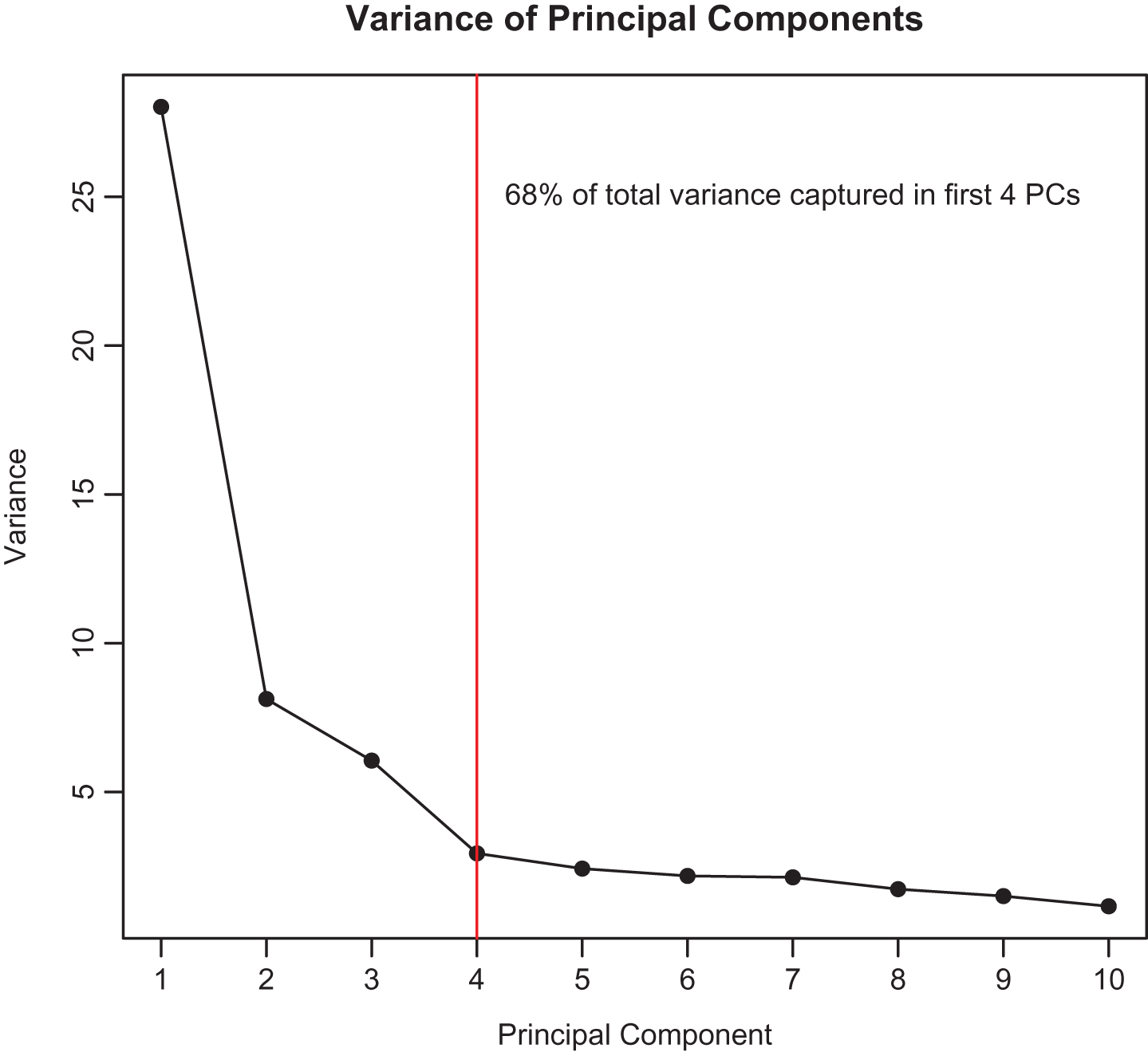
Fig.2
Categorized loading coefficients for all statistics (color online).
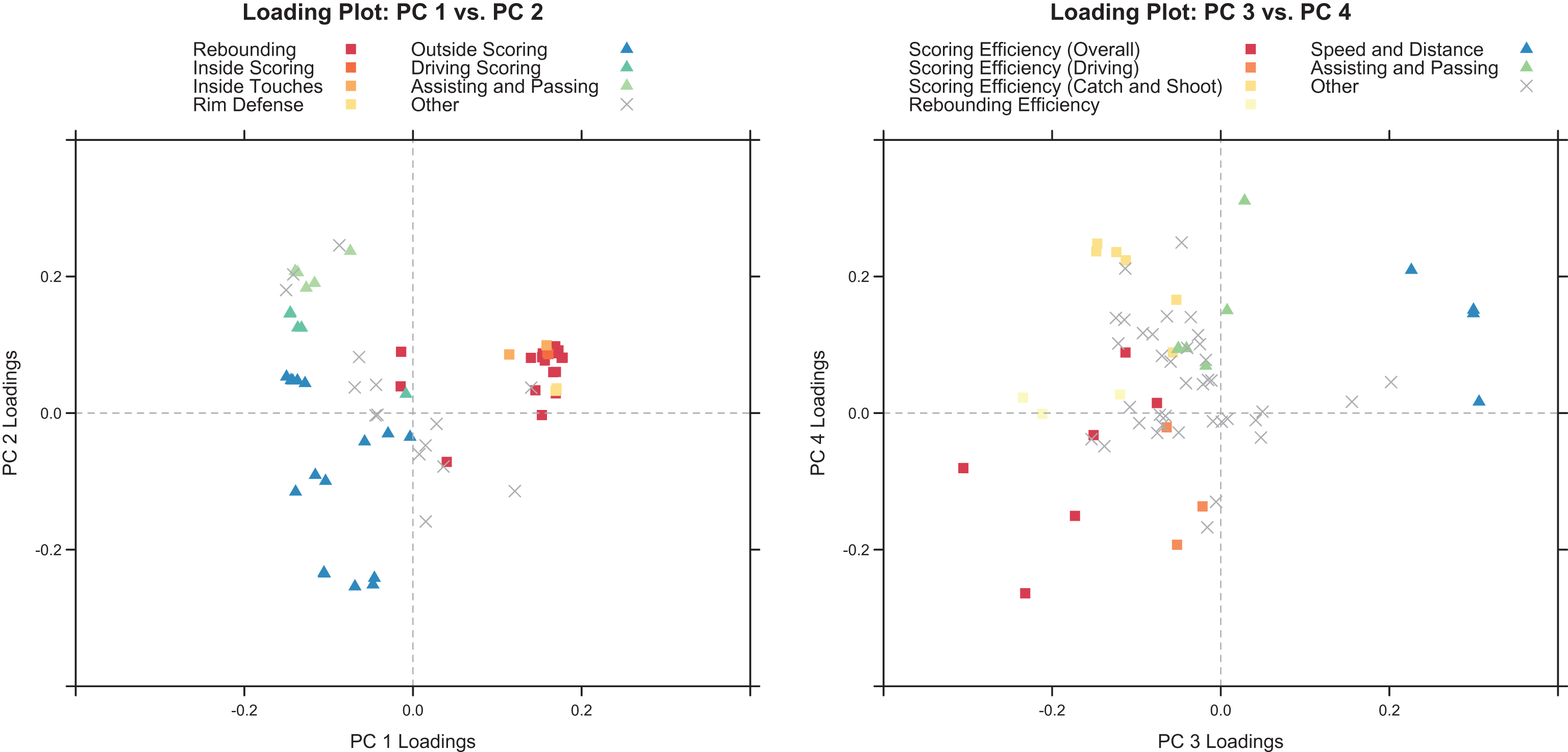
Fig.3
Player PC scores for first four components (color online).
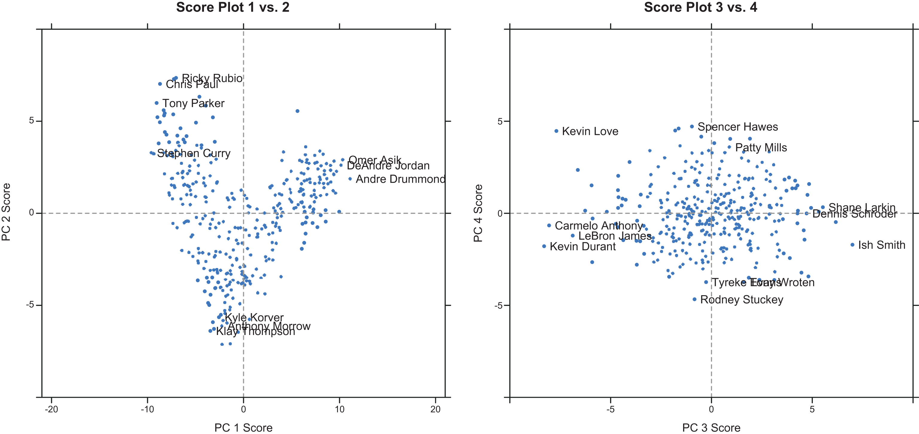
Fig.4
Team average PC scores vs. 2013-2014 regular season winning percentage (color online).
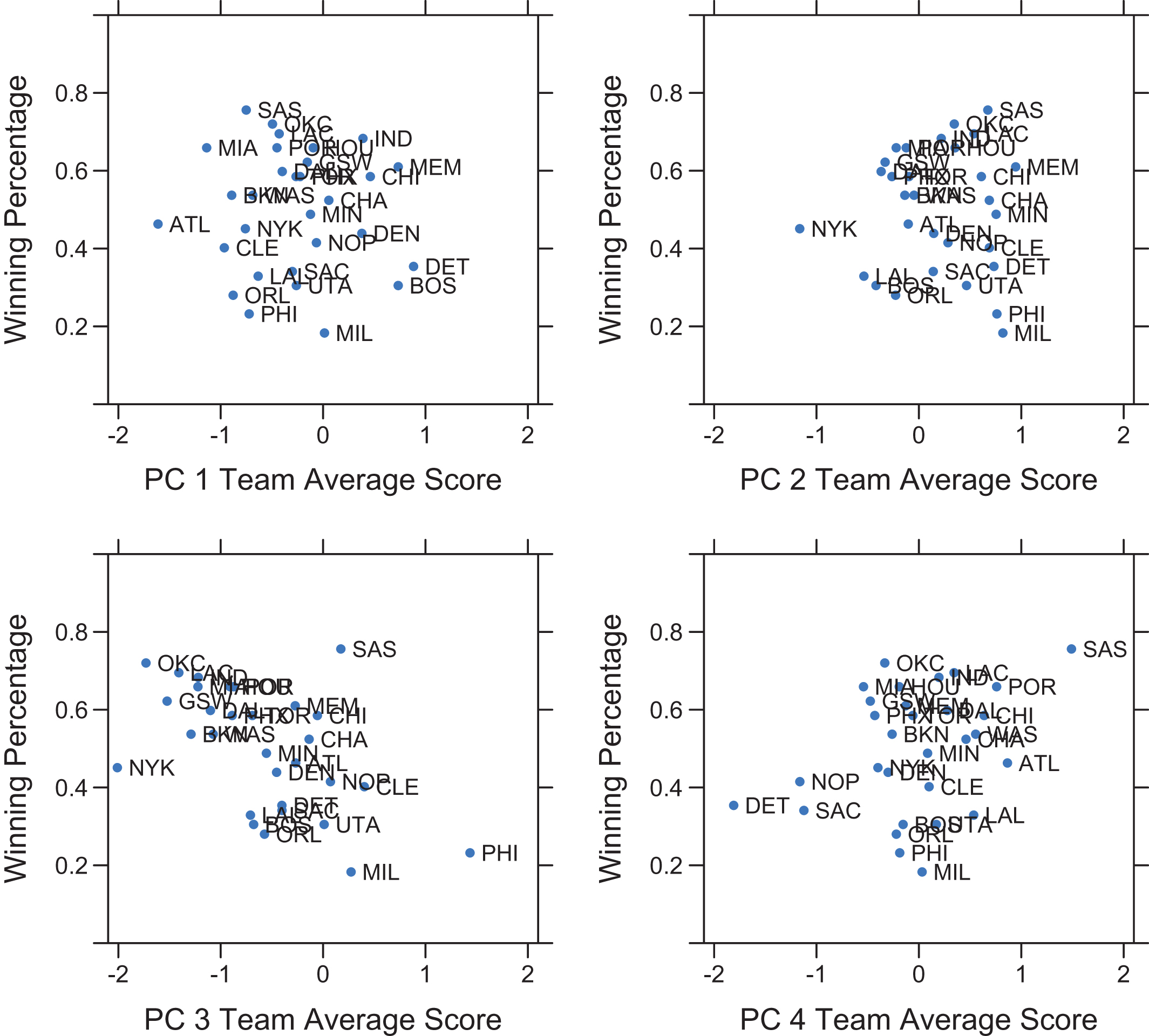
Fig.5
Team average PC 3 scores by regular season winning percentage. Point size determined by regression-weighted sum of PC 2 and PC 4 scores (color online).
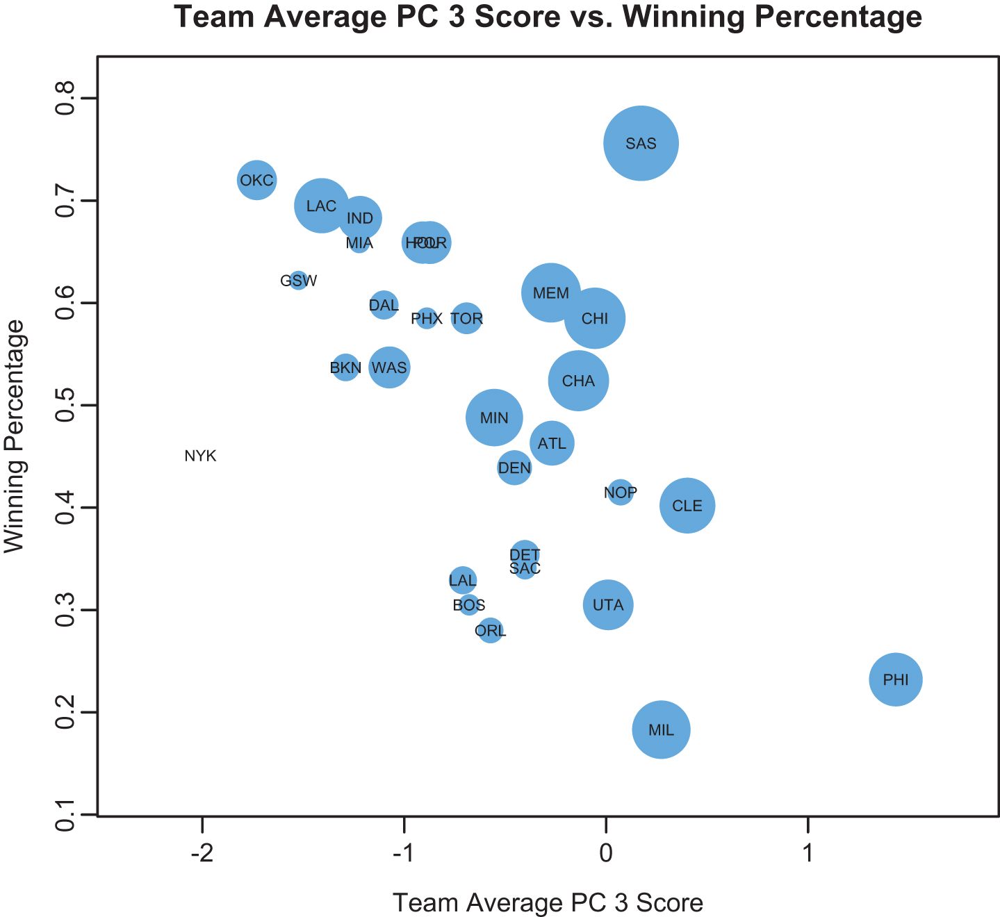
Fig.6
Player PC scores for first four components for Tony Parker comparison (color online).
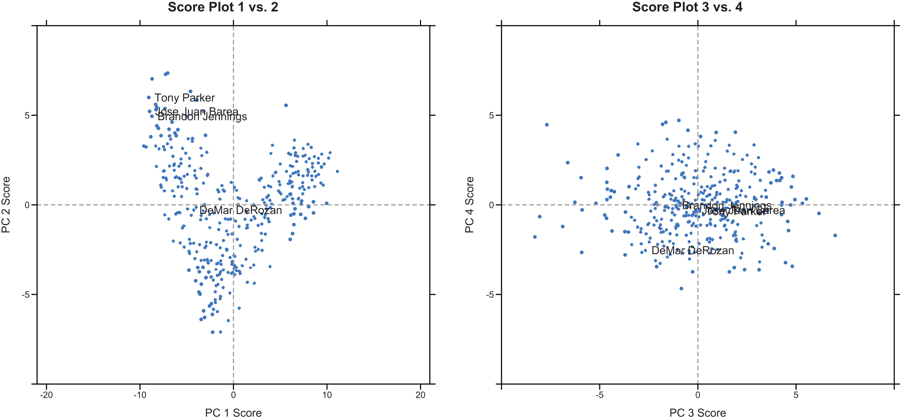
Fig.7
Player PC scores for first four components for Anthony Morrow comparison (color online).
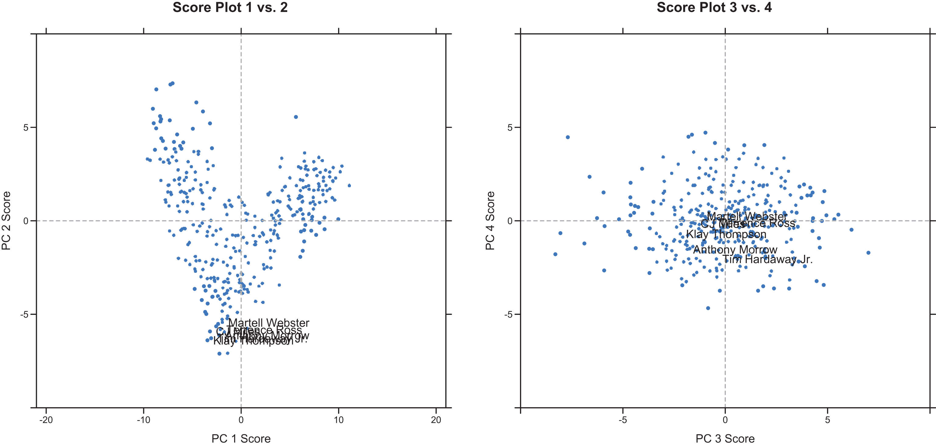
Table 1
Top 10 largest positive(left) and negative(right) loadings for PC 1 (per 48 minutes unless stated otherwise)
| Loading | Statistic | Loading | Statistic |
| 0.178 | Contested Rebounds | –0.150 | Front Court Touches |
| 0.176 | Rebound Opportunities | –0.150 | Pull Up Shot Attempts |
| 0.173 | Offensive Rebounds | –0.146 | Drives |
| 0.172 | Total Rebounds | –0.146 | Team Driving Points |
| 0.171 | Contested Offensive Rebounds | –0.145 | Pull Up Points |
| 0.170 | Opponent Shot Attempts at the Rim | –0.143 | Pull Up Made Shots |
| 0.170 | Contested Defensive Rebounds | –0.142 | Time of Possession |
| 0.169 | Uncontested Rebounding Efficiency | –0.140 | Assist Opportunities |
| 0.169 | Opponent Made Shots at the Rim | –0.139 | Catch and Shoot 3-Point Shooting Efficiency |
| 0.169 | Offensive Rebound Opportunities | –0.137 | Points Created by Assists |
Table 2
Top 5 largest positive(left) and negative(right) loadings for PC 2 (per 48 minutes unless stated otherwise)
| Loading | Statistic | Loading | Statistic |
| 0.246 | Touches | –0.254 | Catch and Shoot Points |
| 0.237 | Passes | –0.251 | Catch and Shoot Attempts |
| 0.208 | Assist Opportunities | –0.242 | Catch and Shoot Made Shots |
| 0.206 | Assists | –0.235 | Catch and Shoot 3-Point Attempts |
| 0.206 | Points Created by Assists | –0.234 | Catch and Shoot 3-Point Made Shots |
Table 3
Top 5 largest positive(left) and negative(right) loadings for PC 3 (per 48 minutes unless stated otherwise)
| Loading | Statistic | Loading | Statistic |
| 0.306 | Average Defensive Speed | –0.305 | Points |
| 0.300 | Distance | –0.235 | Rebounding Efficiency |
| 0.300 | Average Speed | –0.232 | Points per Touch |
| 0.226 | Average Offensive Speed | –0.212 | Defensive Rebounding Efficiency |
| 0.202 | Opponent Points at the Rim | –0.173 | Points per Half Court Touch |
Table 4
Top 5 largest positive(left) and negative(right) loadings for PC 4 (per 48 minutes unless stated otherwise)
| Loading | Statistic | Loading | Statistic |
| 0.311 | Passes | –0.264 | Points per Touch |
| 0.250 | Touches | –0.193 | Drives |
| 0.248 | Catch and Shoot Made Shots | –0.167 | Driving Shot Attempts |
| 0.237 | Catch and Shoot Shooting Efficiency | –0.151 | Points per Half Court Touch |
| 0.236 | Catch and Shoot Points | –0.137 | Team Driving Points |
Table 5
Coefficient estimates in regression of team average PC scores on winning percentage (R2 = 0.59)
| Term | Coefficient | Std Error | p-value |
| Intercept | 0.35 | 0.04 | <0.001 |
| PC 1 Score | –0.01 | 0.04 | 0.758 |
| PC 2 Score | 0.17 | 0.06 | 0.005 |
| PC 3 Score | –0.20 | 0.04 | <0.001 |
| PC 4 Score | 0.09 | 0.03 | 0.013 |
Table 6
Players with lowest SDI compared with Tony Parker and 2013-2014 salary from http://www.basketball-reference.com/
| Player | SDI | Salary |
| Jose Juan Barea (MIN) | 0.7 | $4,687,000 |
| Brandon Jennings (DET) | 2.8 | $7,655,503 |
| Mike Conley (MEM) | 5.5 | $8,000,001 |
| Ty Lawson (DEN) | 5.9 | $10,786,517 |
| Jeff Teague (ATL) | 6.1 | $8,000,000 |
Table 7
Selected statistics for comparison (per 48 minutes unless stated otherwise)
| Statistic | Parker | Barea | Jennings | DeRozan |
| Points | 27.1 | 21.5 | 21.7 | 28.5 |
| Catch and Shoot Points | 2.5 | 3.0 | 3.0 | 5.8 |
| Driving Points | 10.3 | 8 | 4.2 | 6.1 |
| Assist Opportunities | 19.4 | 20.5 | 21 | 10.4 |
| Assist Points Created | 21.9 | 22.5 | 23.7 | 12.6 |
| Touches | 123 | 121 | 113 | 76 |
| Passes | 90 | 89 | 84 | 43 |
Table 8
Players with lowest SDI compared with Anthony Morrow and 2013-2014 salary from http://www.basketball-reference.com/
| Player | SDI | Salary |
| Klay Thompson (GSW) | 2.3 | $2,317,920 |
| CJ Miles (CLE) | 2.9 | $2,225,000 |
| Tim Hardaway Jr. (NYK) | 3.0 | $1,196,760 |
| Terrence Ross (TOR) | 3.8 | $2,678,640 |
| Martell Webster (WAS) | 4.1 | $5,150,000 |
Table 9
Selected statistics for comparison (per 48 minutes unless stated otherwise)
| Statistic | Morrow | Thompson | Miles | Hardaway Jr. | Ross | Webster |
| Catch and Shoot Points | 9.7 | 12.3 | 11.4 | 9.3 | 10.4 | 9.7 |
| Points per Touch | 0.45 | 0.48 | 0.40 | 0.37 | 0.38 | 0.28 |
| Passes | 26.3 | 25.1 | 36.9 | 35.3 | 31.6 | 43.5 |
Table 10
Significant statistic loadings for Principal Component 1
| Statistic | Loading |
| Contested Rebounds | 0.178 |
| Rebounding Opportunities | 0.176 |
| Offensive Rebounds | 0.173 |
| Total Rebounds | 0.172 |
| Contested Offensive Rebounds | 0.171 |
| Opponent Field Goal Attempts at the Rim | 0.17 |
| Contested Defensive Rebounds | 0.17 |
| Uncontested Rebounding Percentage | 0.169 |
| Opponent Field Goal Makes at the Rim | 0.169 |
| Offensive Rebounding Opportunities | 0.169 |
| Defensive Rebounding Opportunities | 0.166 |
| Close Points | 0.161 |
| Close Attempts | 0.159 |
| Close Touches | 0.158 |
| Defensive Rebounds | 0.156 |
| Uncontested Rebounds | 0.154 |
| Uncontested Offensive Rebounds | 0.153 |
| Uncontested Defensive Rebounding Percentage | 0.153 |
| Uncontested Offensive Rebounding Percentage | 0.145 |
| Blocks | 0.14 |
| Uncontested Defensive Rebounds | 0.14 |
| Points per Half Court Touch | 0.121 |
| Elbow Touches | 0.114 |
| Catch and Shoot Effective Field Goal Percentage | -0.104 |
| Catch and Shoot Attempts | -0.105 |
| Catch and Shoot Makes | -0.106 |
| Pull Up 3-Point Percentage | -0.116 |
| Secondary Assists | -0.117 |
| Free Throw Assists | -0.127 |
| Pull Up 3-Point Makes | -0.128 |
| Driving Points | -0.132 |
| Driving Attempts | -0.137 |
| Assists | -0.137 |
| Pull Up 3-Point Attempts | -0.137 |
| Points Created From Assists | -0.137 |
| Catch and Shoot 3-Point Percentage | -0.139 |
| Assist Opportunities | -0.14 |
| Time of Possession | -0.142 |
| Pull Up Makes | -0.143 |
| Pull Up Points | -0.145 |
| Team Driving Points | -0.146 |
| Drives | -0.146 |
| Pull Up Attempts | -0.15 |
| Front Court Touches | -0.15 |
Table 11
Significant statistic loadings for Principal Component 2
| Statistic | Loading |
| Touches | 0.246 |
| Passes | 0.237 |
| Assist Opportunities | 0.208 |
| Assists | 0.206 |
| Points Created From Assists | 0.206 |
| Time of Possession | 0.203 |
| Secondary Assists | 0.19 |
| Free Throw Assists | 0.183 |
| Front Court Touches | 0.18 |
| Team Driving Points | 0.147 |
| Drives | 0.146 |
| Driving Attempts | 0.125 |
| Driving Points | 0.125 |
| Points per Half Court Touch | -0.114 |
| Catch and Shoot 3-Point Percentage | -0.115 |
| Points per Touch | -0.159 |
| Catch and Shoot 3-Point Makes | -0.234 |
| Catch and Shoot 3-Point Attempts | -0.235 |
| Catch and Shoot Makes | -0.242 |
| Catch and Shoot Attempts | -0.251 |
| Catch and Shoot Points | -0.254 |
Table 12
Significant statistic loadings for Principal Component 3
| Statistic | Loading |
| Average Defensive Speed | 0.306 |
| Distance | 0.3 |
| Average Speed | 0.3 |
| Average Offensive Speed | 0.226 |
| Opponent Points at the Rim | 0.202 |
| Close Shooting Percentage | 0.156 |
| Pull Up 3-Point Makes | -0.108 |
| Catch and Shoot Effective Shooting Percentage | -0.113 |
| Effective Shooting Percentage | -0.113 |
| Catch and Shoot Attempts | -0.113 |
| Defensive Rebounds | -0.114 |
| Offensive Rebounding Percentage | -0.119 |
| Elbow Touches | -0.122 |
| Catch and Shoot Points | -0.124 |
| Uncontested Defensive Rebounds | -0.124 |
| Pull Up Attempts | -0.138 |
| Catch and Shoot Makes | -0.146 |
| Catch and Shoot Percentage | -0.148 |
| Pull Up Points | -0.151 |
| Pull Up Makes | -0.153 |
| Points per Half Court Touch | -0.173 |
| Defensive Rebounding Percentage | -0.212 |
| Points per Touch | -0.232 |
| Rebounding Percentage | -0.235 |
| Points | -0.305 |
Table 13
Significant statistic loadings for Principal Component 4
| Statistic | Loading |
| Passes | 0.311 |
| Touches | 0.25 |
| Catch and Shoot Makes | 0.248 |
| Catch and Shoot Percentage | 0.237 |
| Catch and Shoot Points | 0.236 |
| Catch and Shoot Effective Shooting Percentage | 0.224 |
| Catch and Shoot Attempts | 0.212 |
| Average Offensive Speed | 0.209 |
| Catch and Shoot 3-Point Makes | 0.166 |
| Distance | 0.151 |
| Secondary Assists | 0.15 |
| Average Speed | 0.146 |
| Defensive Rebounding Opportunities | 0.142 |
| Catch and Shoot 3-Point Attempts | 0.141 |
| Uncontested Defensive Rebounds | 0.139 |
| Defensive Rebounds | 0.137 |
| Uncontested Rebounds | 0.117 |
| Contested Defensive Rebounds | 0.115 |
| Opponent Makes at the Rim | 0.114 |
| Elbow Touches | 0.102 |
| Opponent Attempts at the Rim | 0.101 |
| Drives | -0.13 |
| Team Driving Points | -0.137 |
| Points per Half Court Touch | -0.151 |
| Driving Attempts | -0.167 |
| Drives | -0.193 |
| Points per Touch | -0.264 |


