
The ebb and flow of official calls in water polo
Abstract
Defensive fouls play an important role in elite men’s water polo generating over half of all goals. Despite their importance, little is known about the relationship between foul calling patterns and other game-state variables in the sport. Here we apply a sequence of hierarchical mixed logistic regression models on data from major tournaments in 2012–2014 to study such relationships and find a number of significant biases in foul calling rates. Offensive teams who are winning/tied are about 31% less likely to draw a defensive foul and 32% more likely to get called for an offensive foul than teams who are losing. The magnitude of losing team bias tends to increase over the course of a game, but is not significantly affected by the size of the lead. A team’s odds of getting called for a foul also increase by about 10% for each consecutive goal scored or foul called in their favor. These biases persist across different offensive and defensive tactical decisions and tournaments suggesting that they are widespread and that it is referees, rather than teams, who are responsible for a lack of independence in water polo foul calling rates.
1Introduction
Fans, players, and coaches alike are well acquainted with the important role played by officiating in sports. A call made (or missed) at a critical moment can drastically alter the evolution of a game and as a consequence, investigating causes, instances, and impacts of foul calling bias is an important topic in sports analytics. The most extensively researched factor influencing referee decisions is home team bias where the literature suggests that not only does home team bias exist, but that its effect can be amplified by external factors such as crowd noise or whether a game is nationally televised; see Neville and Holder (1999) for a survey of results on this topic. In contrast, other studies have focused on how various game-state factors, such as previous calling or scoring patterns, can influence referee decisions. For example, studies of foul calling patterns in NCAA basketball suggest that referees tend to favor the losing team, but also exhibit “sequential bias” in their calls, meaning referees tend to downplay consecutive calls against the same team (Anderson and Pierce (2009); Noecker and Roback (2012)). Similar sequential biases have been observed in soccer penalty kick calls (Plessner and Betsch (2001)). A final example occurs in baseball where it has been shown that strike count can significantly impact an umpire’s “strike zone”, with a smaller strike zone for 0-2 counts than 3-0 counts (Moskowitz and Wertheim (2011); Green and Daniels (2014)).
This study extends previous research on referee bias by examining foul calling patterns in the sport of water polo. There are two kinds of major fouls in water polo: exclusions, in which a defensive player is temporarily excluded from play resulting in a 20 second 6 on 5 power play for the offense, and penalty shots, in which a severe goal-preventing infraction against the defense results in a penalty shot. These two types of fouls play an undisputedly important role in the sport. For example, Fig. 1 below shows the distribution of goals scored from 68 elite men’s water polo contests spanning 2012–2014. Notice that power plays and penalty shots together account for about 56% of all goals scored in these games.
Considering the importance of exclusions and penalty shots in generating goals, one would expect that the number of foul opportunities received by each team is a good classifier of the outcome of water polo games with winning teams receiving more opportunities than losing teams. Recent research, however, has shown that there is no significant difference between the number of exclusion opportunities obtained by winning and losing teams in elite men’s water polo with slightly more than 50% of all games ending with more opportunities for the losing team (Graham and Mayberry (2014)). This counterintuitive result may suggest that water polo referees follow the principle, stated in Askins (1978), of being “fair” (giving equal opportunities to both teams) as opposed to being “objective” (calling fouls based on severity of infractions alone). This paper aims to investigate game-state factors which affect foul calling rates in water polo using game data from three recent international contests: the 2012 Olympics, the 2013 World Championships, and the 2014 European Championships. In addition to the two major types of defensive fouls, we also include offensive foul rates in our analysis. While there have been a number of previous studies which investigate the impact of major fouls on the outcome of water polo contests (Enomote et al. (2003); Hughes et al. (2006); Escalante et al. (2011); Escalante et al. (2012); Lupo et al. (2012); Graham and Mayberry (2014)), this is the first study which takes a dynamic look at foul calling patterns in the sport and seeks to identify situations in which a team’s chances of drawing a foul may significantly differ from their baseline rates. We conclude by exploring whether statistically significant foul calling biases can be explained by differences in playing styles or whether referee bias is a more likely explanation for these effects.
2Results
2.1Data Collection
Data was obtained from 68 elite men’s water polo games including 23 from the 2012 London Olympics (henceforth Oly), 25 from the 2013 World Championships (WC), and 20 from the 2014 European Championships (EC). This data accounts for about 57% of all games played in these three tournaments including all playoff games as well as select games from the preliminary rounds between playoff teams; see Table 1 for a complete list of all teams involved. Games were filmed from mid-court by the first author and other representatives of Team USA water polo. While camera position varied, all twelve players and the defending goalie were kept in frame at all times. The recorded tapes were later viewed by the first author or one of his assistants and play by play game logs were recorded summarizing the outcomes of all possessions in the contests. Information transcribed about each possession included the team on offense, the offensive tactic employed (see Table 3 below), the defensive tactic employed, and the result (goal, missed shot, exclusion, penalty shot, turnover, offensive foul, or rebound). Tactics were classified according to the heuristics described in the appendix of Graham and Mayberry (2014) with the tactics drive, new center, pick, and post-up combined into a single category of movement based tactics for the purposes of analysis. Games were mostly played in neutral locations (the only exceptions were games from the 2013 Championships involving Spain), but with one team assigned to wear home caps (the Dark team) and the other to wear traditional away caps (the White team).
2.2Variables and definitions
Following Kubatko et al. (2007), we define a possession as the period of time from when a particular team takes offensive control of the ball until offensive control returns to the opposing team. Overall, our data set includes 4625 possessions (1556 from Oly, 1766 from WC, and 1303 from EC). Figure 2 shows that the distribution of the number of possessions per game is roughly symmetric (median = 67, mean = 68 possessions per game) with 50% of all games having between 64 and 70 possessions and 90% of all games having between 60 and 77 possessions.
As mentioned in the introduction, there are two major defensive fouls which can be called by water polo referees in a particular possession:
(1) An exclusion in which a player on the defensive team is temporarily excluded from play resulting in a 20 second 6 on 5 power play advantage for the offense.
(2) A penalty shot in which the offensive team is awarded a single penalty shot at the goal.
Referees can also call offensive fouls in which possession of the ball is immediately awarded to the defensive team. Table 2 and Fig. 2 below summarize and compare statistics related to all three major types of fouls.
To investigate foul calling rates, we define two binary variables Dij and Oij which record a 1 if a defensive or offensive foul, respectively, was called during possession i of game j in our database and record a 0 otherwise. We then define the Defensive Foul Rate (DFR) corresponding to a particular situation or game scenario, as the fraction of such situations which resulted in a defensive foul being called and make a similar definition for the Offensive Foul Rate (OFR). For example, if we wish to compute the DFR for possessions in which the offensive team was losing, we would perform the computation
Note that it is possible to obtain a defensive foul followed by an offensive foul in a given possession, but this does not affect the analysis which follows as we run two separate models for defensive and offensive rates. It is also possible that two defensive fouls can be called in different offensive sequences during a single possession, but this is a rare event which occurs in only 0.6% of all possessions in our database and hence, we ignore such double events in our analysis. Figure 3 compares DFR and OFR across all three events in the database. Overall, about 31% of all possessions contained a defensive foul and 11% contained an offensive foul with WC having the lowest foul calling rates of the three events.
The variables Dij and Oij will be used as dependent variables in our analysis of foul calling rates. In Anderson and Pierce (2009), the authors’ analyzed foul calling biases in basketball using a dependent binary variable FH which was 1 if a particular foul went against the home team and 0 if it went against the away team. FH focuses on analyzing the fraction of fouls which go against the home team while our dependent variables focus on the fraction of possessions which result in a foul. Both have merit, however, we focus here on the latter because we are interested in how various independent variables impact the probability of drawing a foul in a given possession.
We will distinguish between three different classes of independent variables in this analysis:
(A) Game-State: variables which relate to the current state of the game during a possession and dynamically evolve over the course of a game (eg. game-time, scoring momentum, whether the offensive team is losing or winning).
(B) Location: variables which relate to game location (Oly, WC, or EC).
(C) Player Choice: variables which relate to choices made by the players during a posses-sion (eg. offensive or defensive play selection).
Our primary interest is in studying the association between foul calling rates and game-state variables. Location variables are included to ensure that any observed effects of game-state variables are uniform across different tournaments. Variables from group (C), while of interest in their own right, serve as controls in our analysis to ensure that any correlations found between foul calling rates and game-state variables cannot be explained by differences in team play and are significant across different offensive and defensive choices. In fact, Graham and Mayberry (2014) showed that certain offensive tactics (such as center and counterattack) are more likely than others to lead to defensive fouls. One might also expect that a press defense is more likely to lead to a foul being called than a more conservative defense such as a zone. Figure 4 compares the distributions of play selections for different offensive states. Since losing and winning/tied teams do tend to exhibit highly significant differences in play selections on defense (
2.3Statistical models and methods
Mixed effect binary logistic regression with a logit link function was used to determine the extent to which foul calling rates depend on the 11 variables in Table 3. Defensive and offensive foul rates were analyzed separately using a sequence of three hierarchical models, each adding additional independent variables. Random effects for Game, Offensive, and Defensive team were included at each level although the estimated variability in such effects was small; see Table 4. The “null” model was that foul calling rates were independent of game-state, location, and player choice variables. The next level of models included all six game-state variables, the primary effects of interest in our analysis. The final level dropped insignificant game-state variables and added both location and player choice variables to ensure that any significant game-state variables in level 1 were still significant after accounting for these confounding effects. For independent categorical variables with k options, one category was arbitrarily chosen as the base category and binary dummy variables were created to determine the impact of the other k - 1 categories. Standard Wald z-tests for nonzero coefficients in the logistic model were used to identify independent variables which significantly impacted foul calling rates (significance level α = 0.05). Likelihood Ratio Tests were employed to determine if higher level models in the hierarchy significantly improved upon lower level models and the resulting χ2 (Deviance) test statistics are reported below along with the corresponding p-values. Select interactions between variables of interest were also analyzed using this hierarchical approach. All statistical analysis was performed using the statistical software R, v3.2.2. The glmer function from the lme4 package was used to compute model coefficients and errors.
3Results and discussion
Tables 5 and 6 below show the fitted parameters from our models for defensive and offensive foul rates, respectively. In both scenarios, the level 1 models were significant improvements over the null models (DFR:
State, foul, and scoring momentum had similar associations with offensive calling rates: an offensive foul was significantly more likely to be called if the offensive team was winnign/tied or had momentum in their favor. In contrast to defensive fouls, however, offensive rates were not significantly correlated with either game-time or lead, but were negatively correlated with foul differential.
Both level 2 models were significantly better predictors of foul calling rates than their level 1 counterparts (DFR:
Game-time, however, had an interesting interaction with state in modeling defensive foul calling rates. While Fig. 8 below shows that losing team bias was present across the spectrum of a game, there was a moderately significant interaction between these two variables (estimated coefficient of interaction = -0.458, z = -1.786, p = 0.074). In particular, the interaction model predicts that at the beginning of a game, the odds of drawing a defensive foul are only about 12% lower for winning/tied teams as opposed to losing teams, but near the end of the game, the odds of drawing a foul are 44% lower for winning/tied teams. We also tested for an interaction between the state and size of the lead to confirm that losing team bias was equally present in close and unbalanced games and found no significant interaction between these two predictors (
Although the impact of game-state variables is the primary aim of this study, the play selection variables in our model exhibited some noteworthy correlations with defensive and offensive foul rates as well. First, defensive selections were not significantly associated with DFR, but were significantly associated with OFR. Split and zone defenses yielded smaller OFR than press or transition defenses. The offensive team’s choice of attack was significantly associated with both types of foul calls, but in different ways. DFR was higher for what would be considered more aggressive offensive tactics (center, counterattack, double post, and movement) than for more conservative, outside shooting tactics (perimeter and direct shots). OFR was also higher for center, movement, and double post tactics, but in contrast to DFR, was higher for direct shots than for counterattacks or perimeter shots. Thus counterattacks appear to be the best case scenario for an offensive team, yielding high defensive, but low offensive foul calling rates. This observation is not too surprising since counterattacks usually result from “fast break” scenarios in which offensive players greatly outnumber the defensive players on the offensive side of the pool. The fact that center and movement based tactics yield high OFR and DFR is also not surprising since both typically involve even situations with a great deal of player interaction. Somewhat more surprising is the fact that direct shots, which have been suggested as an undervalued tactic in Graham and Mayberry (2014) yield low defensive foul calling rates, but high offensive foul calling rates. Finally, note that the number of plays run in a possession was positively correlated with a team’s chances of drawing a defensive, but not an offensive foul. This may be related to the idea that if an event has a positive probability p of occurring in a single experiment, then the probability of obtaining at least one occurrence in n independent experiments is 1 - (1 - p) n ≥ p. Of course, the outcomes of successive plays will not be completely independent, but the dependencies may be weak enough to ensure that the probability of obtaining at least one successive is a strictly increasing function of the number of plays run.
To address location, our models suggest that offensive foul calling rates were roughly consistent across the three events in our database, but that defensive rates were significantly lower at the WC than the other two events. Figure 6, however, demonstrates that the losing team bias was consistent across the three tournaments. A formal test confirmed that there was no significant interaction between state and event in our model (Defense:
4Conclusions
Our analysis shows that foul calls in water polo are highly dependent upon the state of a game. Losing team bias is particularly prevalent in the sport with offensive teams who are winning/tied being about 31% less likely to get a defensive foul called in their favor and about 32% more likely to get an offensive foul called against them than losing teams. Offensive teams are negatively affected by both scoring and foul calling momentum as well, with the odds of drawing a defensive (offensive) foul decreasing (increasing) by around 10% for each consecutive point scored or foul called against them. Defensive foul calling rates (but not offensive) tend to be higher in close games, decreasing as the size of the lead increases. It also appears that defensive foul rates tend to increase over the course of the game while offensive foul rates remain constant. Table 7 below further elucidates these results by comparing the odds of getting called for a foul in several opposing game scenarios as predicted by our level 2 models. For example, when an offensive team has had two consecutive goals scored against them, the odds of drawing a defensive foul are 100 [1 - exp {4 (-0.110)}]≈36 % greater than when they have scored the previous two goals if we hold all other variablesconstant.
There are two potential explanations for why foul calling rates depend on the game-state variables mentioned above:
(1) Teams commit more fouls when they are winning or have momentum in their favor.
(2) Teams get called for more fouls when they are winning or have momentum in their favor.
In other words, the explanation could either lie with the players (1) or the referees (2). Although we cannot completely rule out (1), the inclusion of player choice variables into our level 2 models provides some evidence in favor of (2) as an explanation: even after we account for differences in offensive and defensive choices, scoring momentum, foul momentum, and state remain significant predictors of foul calling rates on both sides of the pool. Furthermore, there were no significant interactions between state and player choice variables in modeling foul rates suggesting that losing team bias is not an artifact of tactical choices made by teams. We therefore argue that referees are the main source of game-state biases in foul calling rates. In particular, referees consciously or subconsciously tend to favor teams who are losing and attempt to minimize sequential calls against the same team. Since there is no significant interaction between the sign and size of the lead, it would appear that this losing team bias is not just due to a “sympathy” effect which comes into play once a team is down by a certain amount. There was also evidence of an interaction between game-time and game state with losing team bias increasing in magnitude over the progression of a game.
Foul calling biases may help explain why Graham and Mayberry (2014) found that exclusion conversion rate (ECR), defined as the fraction of exclusion opportunities converted to goals, is one of the best classifiers of game outcomes in international men’s water polo while exclusion opportunities is no better than flipping a coin. In fact, the team with a higher exclusion conversion rate wins almost 90% of all contests while the team with more exclusion opportunities loses slightly more than 50% of all contests. The results of this present paper in regard to both losing team effects and sequential biasing further illuminate the importance of this fact. A losing team is more likely to get an exclusion opportunity, but consecutive opportunities are discouraged and hence those team’s which can convert exclusions are at a significant advantage over their opponents.
Although the ratio of observations to variables in our data set is too low to yield a meaningful analysis of all higher order interaction terms, this would be an interesting project for future research. One particularly interesting question is to see how interactions between pairs of game-state variables persist across events. As an example, Fig. 9 suggests that there is a significant interaction between scoring momentum and state at the Olympics and World Championships with scoring momentum being positively correlated with offensive foul calling rates for winning/tied teams, but not losing teams. There appears to be no such interaction at the European Championships, however, and a test for a three-way interaction confirms the significance of these differences (
Another limitation of our analysis is the lack of time specific information related to possessions in our database. For example, we did not have a record of how long each possession lasted and hence, were forced to measure game-time as a fraction of the total number of game possessions which had elapsed by the end of the current possession. As more possession specific water polo data becomes openly available, the impact of possession length and game-time should be reexamined. In addition, to further rule out team play as an explanation for losing team bias, it would be helpful to have a method for quantifying the aggressiveness of a possession. Our player choice variables provide a potential surrogate for the absence of such measurements (press defense could be considered as a more aggressive choice than zone; counterattacks, center plays, and movement based tactics could be considered more aggressive than direct shots and perimeter plays), but cannot account for differences in aggression in the execution of said tactics.
Finally, we would like to mention that the inclusion of random effects for teams and games did not impact our results and that the variance related to these effects was neglible. This suggests that the reported biases are widespread and not restricted to any particular team or game. Consistent with the findings of previously mentioned studies in basketball, soccer, and baseball, game-state based referee biases appear to be a uniform phenomenon in elite men’s water polo, favoring “fair” over “objective” patterns of foul calling behavior. Thus our study extends previous research on officiating call patterns to a new sport and contributes to the growing body of analytic research in water polo.
Acknowledgments
This research was funded in part by Team USA water polo and the Water Polo Analytics Group.
References
1 | Anderson K. and Pierce D., (2009) . Officiating bias: The effect of foul differential on foul calls in ncaa basketball. Journal of Sports Science, 270: (7), 687–694. |
2 | Askins R.L., (1978) . The official reacting to pressure. Referee, 3: , 17–20. |
3 | Enomote I., Suga M., Takahashi M., Komori M., Minami T., Fujimoto H., Saito M., Suzuki S. and Takahashi J., (2003) . A notational match analysis of the 2001 women’s water polo world championships. Proceeding of Biomechanics and Medicine in Swimming IX, Saint-Etienne, University of Saint Etienne, pp. 487–492. |
4 | Escalante Y., Saavedra J.M., Mansilla M. and Tella V., (2011) . Discriminatory power of water polo game-related statistics at 2008 the olympic games. Journal of Sports Sciences, (29), 291–298. |
5 | Escalante Y., Saavedra J.M., Tella V., Mansilla M., Garca-Hermoso A. and Dominguez, (2012) . Water polo game-related statistics in women’s international championships: Differences and discriminatory power. Journal of Sports Science and Medicine, (11), 475–482. |
6 | Graham J. and Mayberry J., (2014) . Measures of tactical efficiency in water polo. Journal of Quantitative Analysis in Sports, 10: (1), 67–79. |
7 | Green E. and Daniels D., (2014) . What does it take to call a strike? three biases in umpire decision making. 8th Annual Sloan-MIT Sports Analytics Conference Proceedings. |
8 | Hughes M., Appleton R., Brooks C., Hall M. and Wyatt C., (2006) . Notational analysis of elitemen’s water-polo. Proceeding of 7th World Congress of Performance Analysis, Szombathely, Hungary, 137–159. |
9 | Justin Kubatko, Dean Oliver, Kevin Pelto and Dan T. Rosenbaum, (2007) . A starting point for analyzing basketball statistics. Journal of Quantitative Analysis in Sports, 3: (3), 516–525. |
10 | Lupo C., Condello G. and Tessitore A., (2012) . Notational analysis of elite men’s water polo related to specific margins of victory. Journal of Sports Science and Medicine, (11), 516–525. |
11 | Noecker C. and Roback P., (2012) . New insights on the tendency of ncaa basketball officials to even out foul calls. Journal of Quantitative Analysis in Sports, 80: (3), 1–23. |
12 | Neville A. and Holder R.L., (1999) . Home advantage in sport: An overview of studies on the advantage of playing at home. Sports Medicine, 280: (4), 221–236. |
13 | Plessner H. and Betsch T., (2001) . Sequential effects in important referee decisions: The case of penalties in soccer. Journal of Sport and Exercise Psychology, 23: , 254–259. |
14 | Tobias J. Moskowitz and Jon Wertheim L., (2011) . Scorecasting: The Hidden Influences Behind How Sports Are Played and Games Are Won. Crown Archetype, New York. |
Figures and Tables
Fig.1
Distribution of goals scored by game situation across 68 games from elite men’s water polo contests in the 2012 Olympics, 2013 World Championships, and 2014 European Championships. Even situations includes all set six on six offensive configurations whereas counterattack includes all fast break or transition situations in which one or more defensive players is still returning to position after a change of possession.
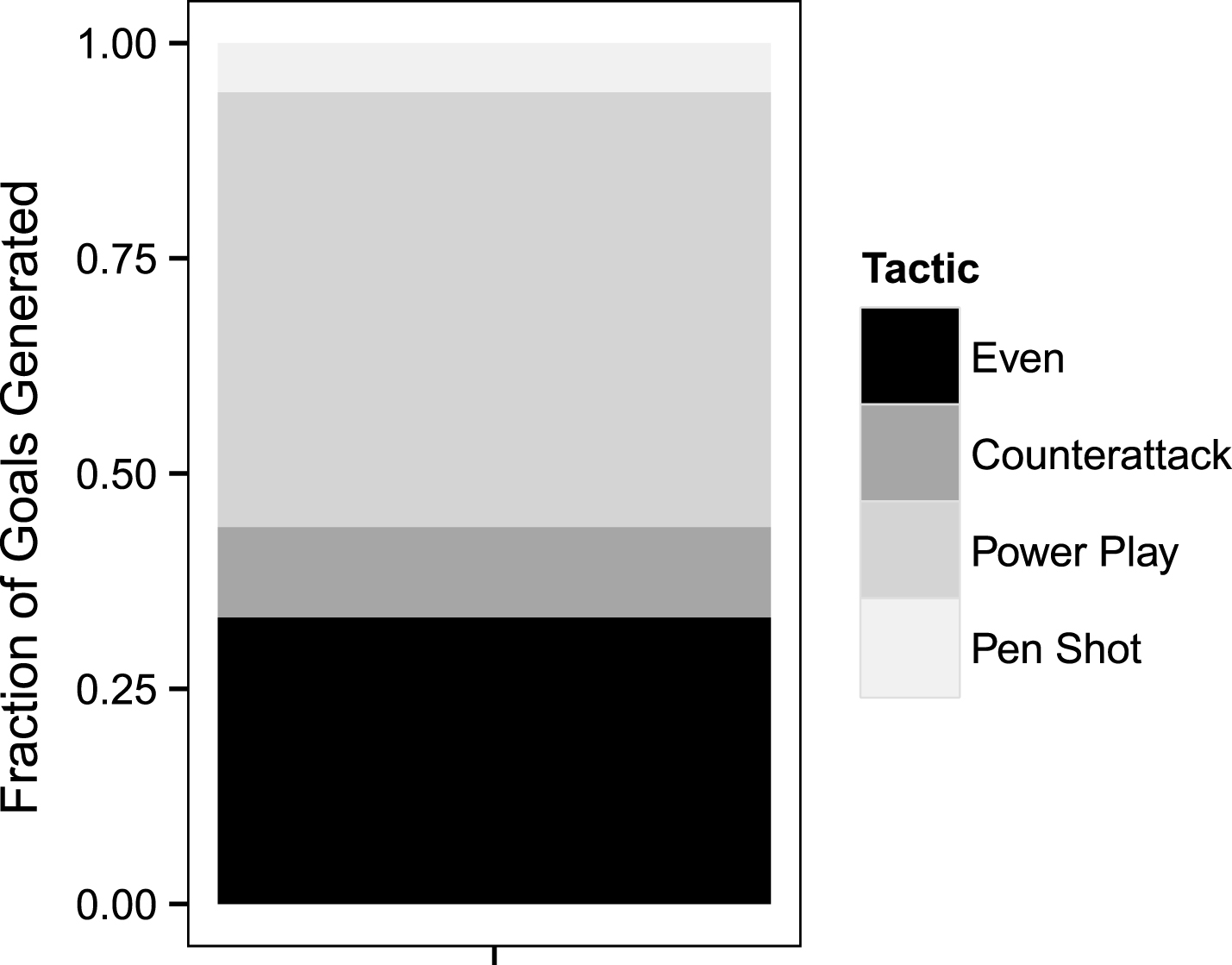
Fig.2
Distribution of the number of possessions (left) and number of fouls (right) across all games in our data set.
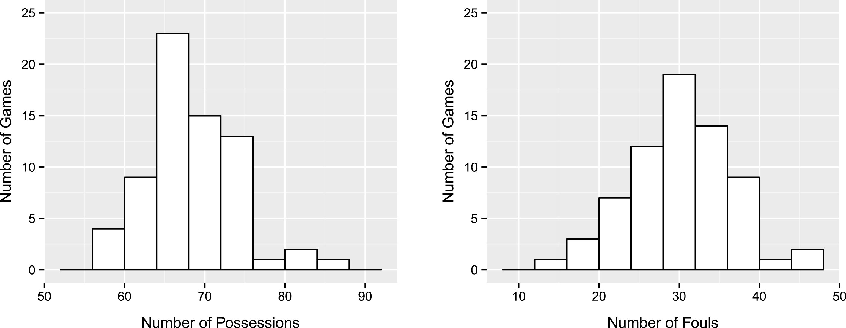
Fig.3
Comparison of the overall DFR (left) and OFR (right) for all three events. Error bars show the respective 95% confidence intervals for each estimate.
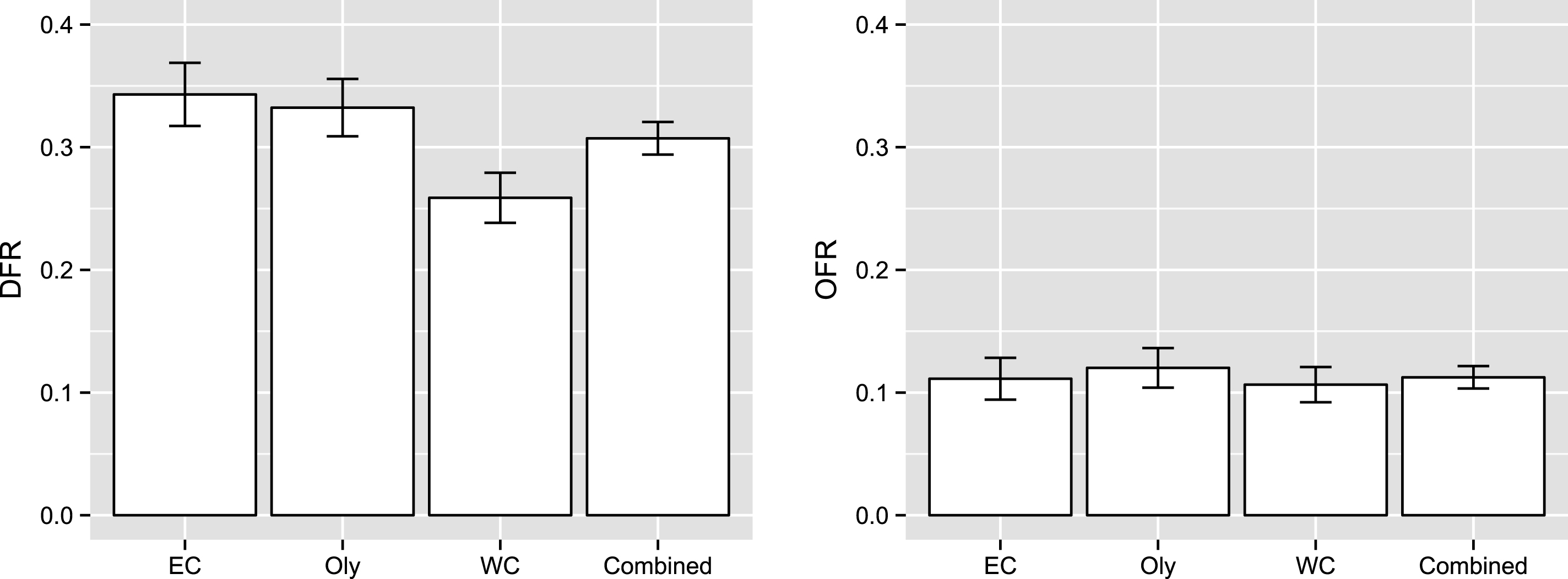
Fig.4
Comparison of offensive play selection (left) and defensive play selection (right) based on whether the team is losing or winning/tied.
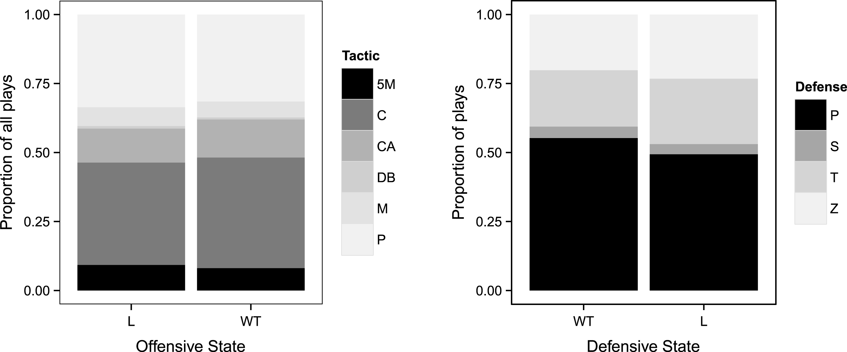
Fig.5
Bar plot demonstrating losing team bias in both defensive (left) and offensive (right) foul calling rates.
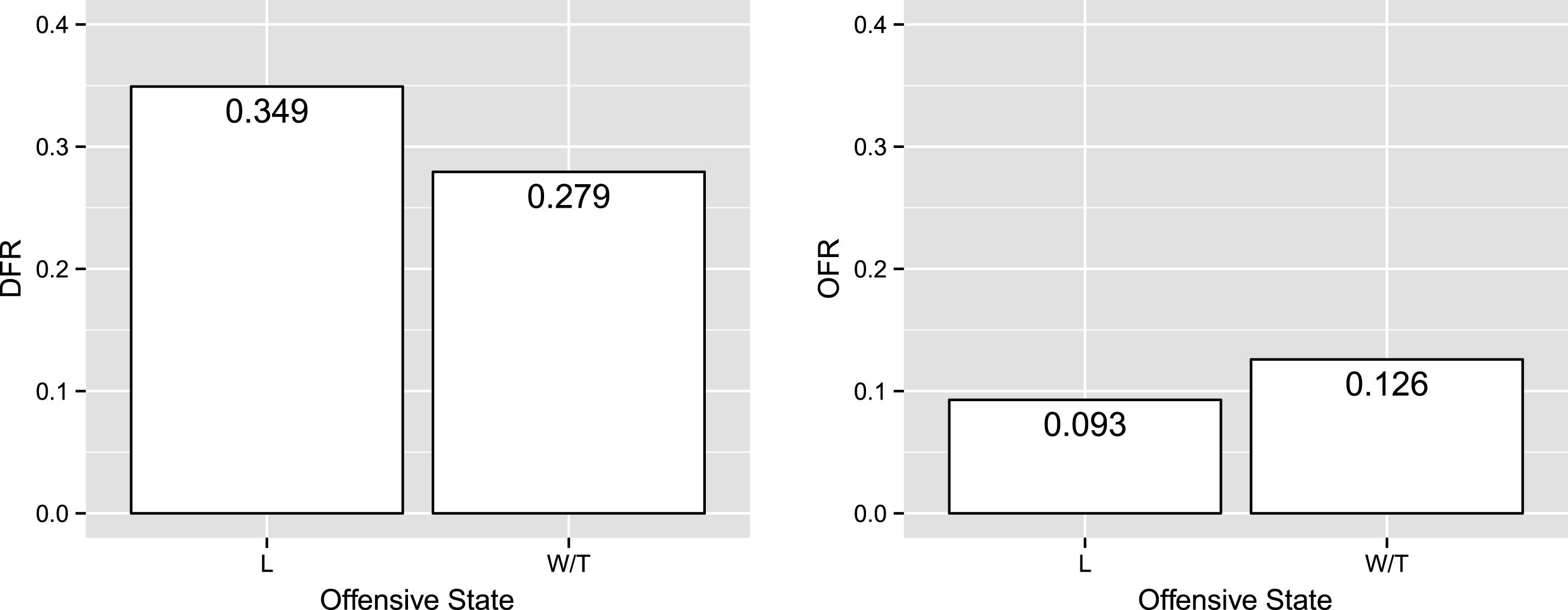
Fig.6
Comparison of DFR across states and events. Defensive foul calling rates were significantly lower at the WC than at the other two events, but there was no significant interaction between event and state in our model.
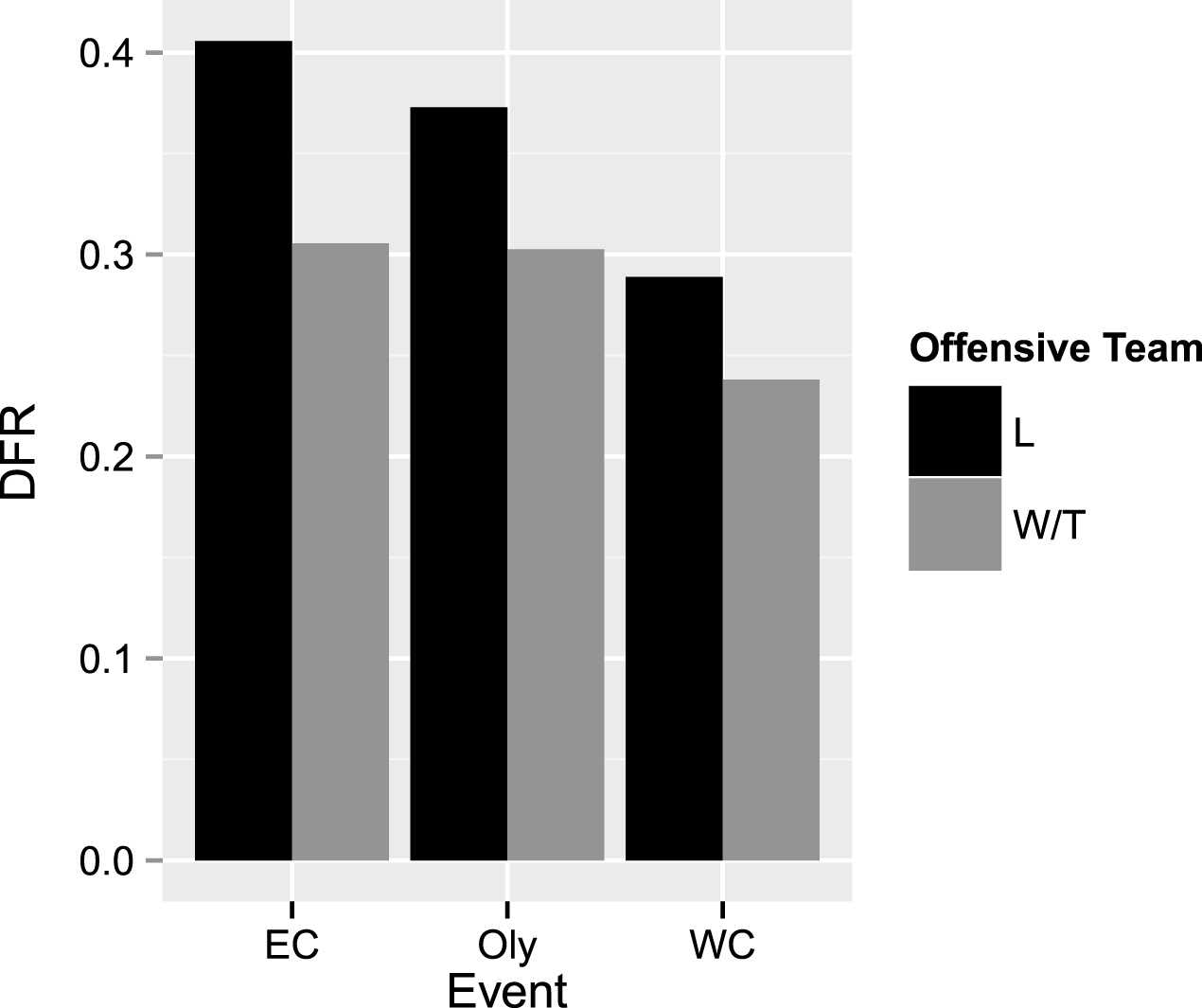
Fig.7
Comparison of DFR for offensive teams who are losing vs. winning/tied across different defensive play selections (left) and offensive attack tactics (right). The blank option in tactics indicates possessions in which no specific tactic was run by the offensive team (the base category).
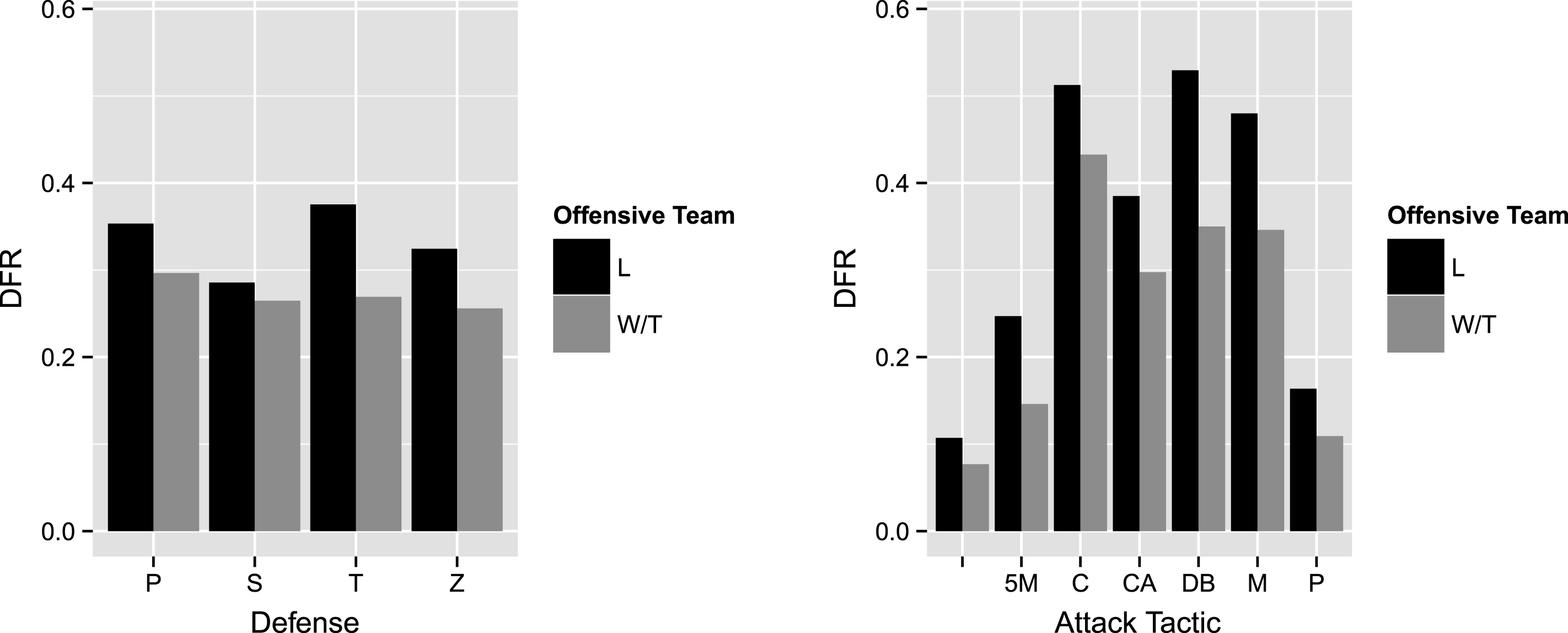
Fig.8
Comparison of DFR for losing and winning/tied teams based on octant of game play (1st half of first quarter, 2nd half of first quarter, etc.). Losing teams have a higher probability of drawing a foul across all octants of game play although there was a moderately significant interaction suggesting that the magnitude of losing team bias may be increasing over the course of a game.
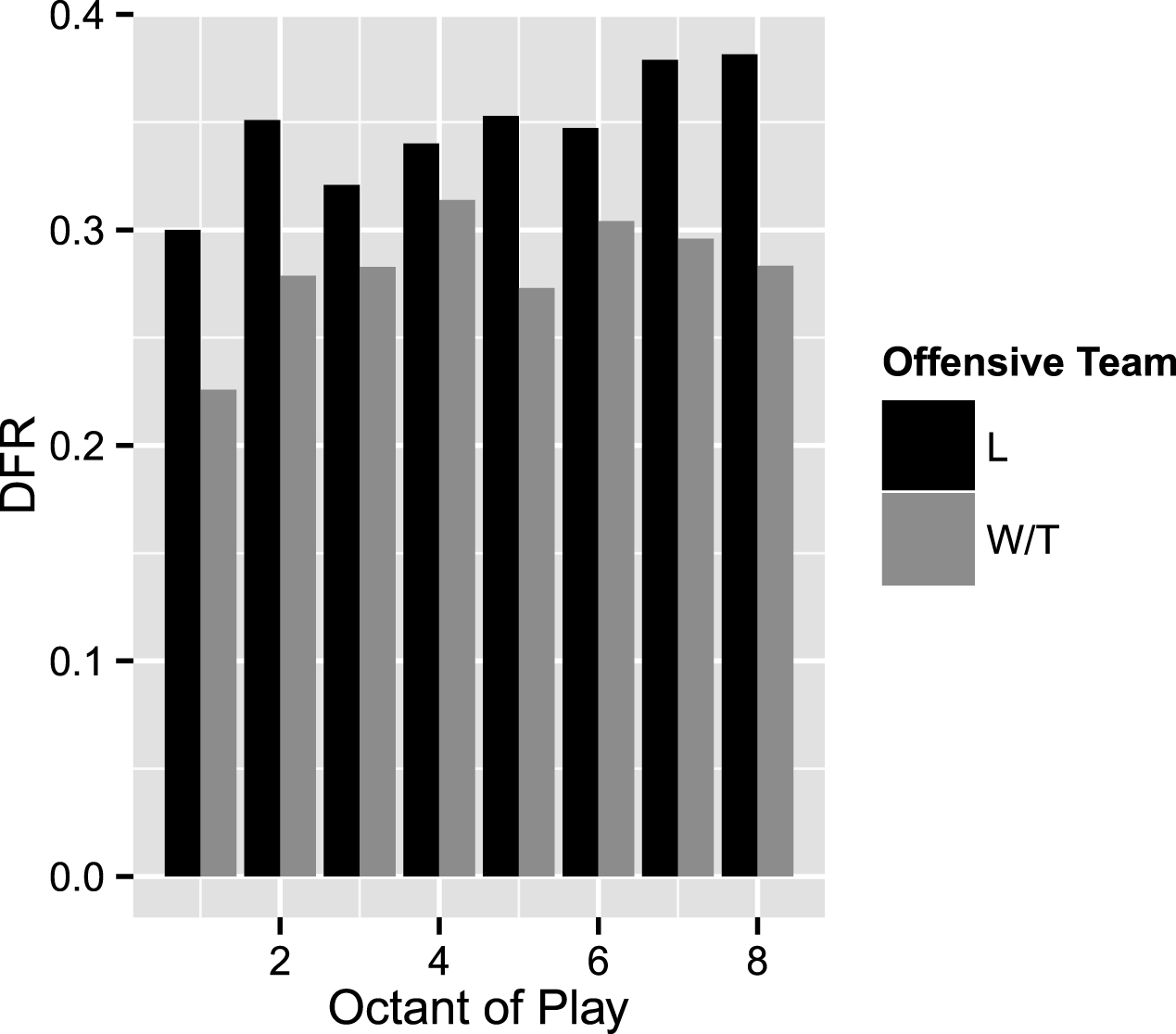
Fig.9
Plots of OFR vs. scoring momentum for the Olympics and World Championships (left) and the European Championships (right) broken down by state to illustrate the three way interaction between scoring momentum, state, and location. In the graph on the left, scoring momentum is positively correlated with OFR only when the offensive team was winning/tied while in the graph on the right there is no correlation between OFR and scoring momentum.
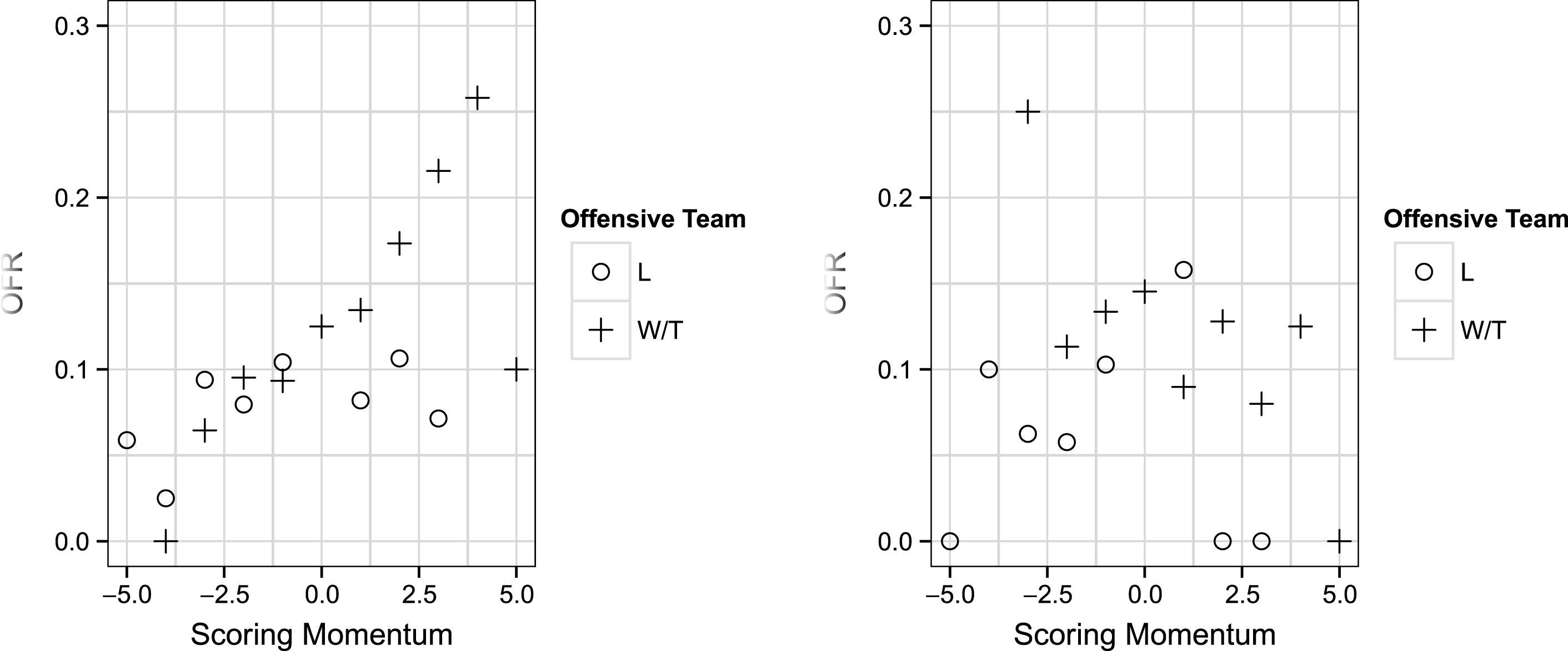
Table 1
Representation of different teams in our database
| Team | Number of Games |
| Australia | 11 |
| Canada | 2 |
| China | 3 |
| Croatia | 15 |
| Germany | 2 |
| Greece | 13 |
| Hungary | 16 |
| Italy | 15 |
| Montenegro | 14 |
| Romania | 8 |
| Serbia | 15 |
| Spain | 14 |
| United States | 8 |
Table 2
Statistics on all three types of fouls considered in this paper.The mean and SD refer to the mean and standard deviation of the number of fouls per game across our data set. Goal conversion rate is defined as the fraction of fouls which resulted in a goalbeing scored on the possession. For penalty shots, this is equivalent to the shooting percentage, but for exclusions, the conversion rate also takes into account goals scored in the current possessionafter an exclusion ends. Goal conversion rates have been shown to be a better metric for measuring the effectiveness of exclusions than shooting percentage alone; see Graham and Mayberry (2014) for details
| Foul | Mean | SD | Goal Conversion Rate (95% CI) |
| Exclusion | 20.691 | 5.509 | 0.475 (0.449, 0.501) |
| Penalty Shot | 1.309 | 2.873 | 0.753 (0.664, 0.842) |
| Offensive | 7.662 | 1.040 | NA |
Table 3
List of all independent variables used in our models. Category (A) refers to game-state, Category (B) refers to location, and Category (C) refers to player choice variables
| Class | Variable | Explanation |
| (A) | State | Binary variable which takes on the value of 1 if the offensive team is winning/tied at the start of the current possession. |
| (A) | Lead | Numeric variable indicating the absolute value of the score differential at the start of the current possession. |
| (A) | Foul Differential | Numeric variable indicating the difference between the number of fouls called in favor of the offensive team and the number of fouls called in favor of the defensive team at the start of the current possession. |
| (A) | Scoring Momentum | Numeric variable indicating the number of consecutive goals which have been scored by the offensive team at the start of the current possession with negative values indicating momentum in favor of the defensive team. |
| (A) | Foul Momentum | Numeric variable indicating the number of consecutive fouls (both offensive and defensive) called in favor of the offensive team at the start of the current possession with negative values indicating momentum in favor of the defensive team. |
| (A) | Game-time | Numeric variable with values in [0, 1] indicating the fraction of all game possessions which have elapsed by the current possession. |
| (B) | Event | Categorical variable specifying the event corresponding to the current possession. The options are EC, Oly, and WC with EC serving as the base category. |
| (C) | Defense | Categorical variable which classifies the defense used in a particular possession. The four options are: Press, Split (between Press and Zone), Transition (ie. counterattack), or Zone with Press acting as the base category. |
| (C) | Attack | Categorical variable which classifies the offensive tactic employed on the initial attack of the possession. The base category is no attack. The other options are 5M Direct Shot (or Free Throw), Center, Counterattack, Double Post, Movement (Drive, Pick, Post-Up, or New Center), and Perimeter Shot. See Graham and Mayberry (2014) for a more complete description of these offensive tactic classifications. |
| (C) | Plays | The number of non-exclusion plays run by the offensive team during the possession. |
Table 4
Standard deviation of random effects from Level 0 (L0), Level 1 (L1), and Level 2 (L2) models. Note that there were a total of 68 games and 14 offensive/defensive teams
| Defensive Fouls | Offensive Fouls | |||||
| L0 | L1 | L2 | L0 | L1 | L2 | |
| Game | 0.277 | 0.223 | 0.203 | 0.000 | 0.000 | 0.000 |
| Off. Team | 0.135 | 0.282 | 0.153 | 0.157 | 0.115 | 0.106 |
| Def. Team | 0.000 | 0.103 | 0.101 | 0.239 | 0.275 | 0.270 |
Table 5
Coefficients and p-values from Wald’s tests in the level 0 (null), level 1, and level 2 logistic models for DFR. Blanks represent terms not included in the model
| Term | Level 0 | Level 1 | Level 2 | |||
| Coeficient | p-value | Coeficient | p-value | Coeficient | p-value | |
| Intercept | –0.844 | <0.001 | –0.845 | <0.001 | –2.414 | <0.001 |
| State | –0.388 | <0.001 | –0.368 | <0.001 | ||
| Lead | –0.089 | 0.001 | –0.092 | 0.001 | ||
| Foul Diff | 0.026 | 0.081 | ||||
| Foul Mom | –0.077 | 0.003 | –0.091 | 0.001 | ||
| Score Mom | –0.110 | <0.001 | –0.115 | <0.001 | ||
| Game-time | 0.488 | <0.001 | 0.722 | <0.001 | ||
| Defense = S | –0.063 | 0.747 | ||||
| Defense = T | –0.131 | 0.315 | ||||
| Defense = Z | –0.057 | 0.541 | ||||
| Attack = 5M | 0.563 | 0.189 | ||||
| Attack = C | 2.084 | <0.001 | ||||
| Attack = CA | 1.779 | <0.001 | ||||
| Attack = DB | 1.994 | <0.001 | ||||
| Attack = M | 1.887 | <0.001 | ||||
| Attack = P | 0.233 | 0.575 | ||||
| Plays | 0.178 | <0.001 | ||||
| Event = Oly | –0.087 | 0.446 | ||||
| Event = WC | –0.361 | 0.002 | ||||
Table 6
Coefficients and p-values from Wald’s tests in the level 0 (null), level 1, and level 2 logistic models for OFR. Blanks represent terms not included in the model
| Term | Level 0 | Level 1 | Level 2 | |||
| Coeficient | p-value | Coeficient | p-value | Coeficient | p-value | |
| Intercept | –2.131 | <0.001 | –2.230 | 0.000 | –4.702 | 0 |
| State | 0.300 | 0.012 | 0.28 | 0.014 | ||
| Lead | 0.028 | 0.425 | ||||
| Foul Diff | –0.072 | 0.001 | –0.073 | 0.001 | ||
| Foul Mom | 0.100 | 0.008 | 0.111 | 0.004 | ||
| Score Mom | 0.081 | 0.012 | 0.104 | 0.001 | ||
| Game-time | –0.271 | 0.148 | ||||
| Defense = S | –0.795 | 0.018 | ||||
| Defense = T | 0.003 | 0.985 | ||||
| Defense = Z | –0.256 | 0.042 | ||||
| Attack = 5M | 2.119 | 0.039 | ||||
| Attack = C | 2.911 | 0.004 | ||||
| Attack = CA | 1.91 | 0.063 | ||||
| Attack = DB | 2.647 | 0.018 | ||||
| Attack = M | 3.122 | 0.002 | ||||
| Attack = P | 1.86 | 0.067 | ||||
| Plays | –0.012 | 0.819 | ||||
| Event = Oly | 0.114 | 0.365 | ||||
| Event = WC | 0.016 | 0.898 | ||||
Table 7
The percent decrease and increase in the odds of getting a defensive a nd offensive foul called, respectively, from Scenario 1 to Scenario 2 as predicted by our level 2 model (holding all other variables constant)
| Scenario 1 | Scenario 2 | Decrease in | Increase in |
| Def Foul Odds | Off Foul Odds | ||
| Offense Losing | Offense Winning/Tied | 31% | 32% |
| Scoring Momentum = -2 | Scoring Momentum = +2 | 37% | 52% |
| Foul Momentum = -2 | Foul Momentum = +2 | 31% | 56% |
| Lead = 0 | Lead = 4 | 31% | None |
| Foul Diff = -2 | Foul Diff = +2 | None | 25% |
| End of game | Start of game | 51% | None |


