
Auxiliary-LSTM based floor-level occupancy prediction using Wi-Fi access point logs
Abstract
Smart city concepts have gained increased traction over the years. The advances in technology such as the Internet of things (IoT) networks and their large-scale implementation has facilitated data collection, which is used to obtain valuable insights towards managing, improving, and planning for services. One key component in this process is the understanding of human mobility behaviour. Traditional data collection methods such as surveys and GPS data have been extensively used to study human mobility. However, a key concern with such data is the protection of user privacy. This study aims to overcome those concerns using Wi-Fi access point logs and demonstrate their utility by creating building occupancy prediction models using advanced machine learning techniques. The floor level occupancy counts and auxiliary variable for a campus building are extracted from the Wi-Fi logs. They are used to develop specifications of Long-Short Term Memory network (LSTM), Auxiliary LSTM (Aux-LSTM), Autoregressive Integrated Moving Average (ARIMA), and Multi-layer Perceptron (MLP) models. The LSTM performed better than the other models and can efficiently capture peak values. Aux-LSTM was shown to increase the reliability in prediction and applicability in the context of facilities management. Results show the effectiveness of the Wi-Fi dataset in capturing trends, providing supplementary information, and highlight the ability of LSTM to adequately model time-series data.
1.Introduction
A smart city is based on human-to-human, human-to-environment, and environment-to-environment interactions. The term environment encompasses the systems, sensors, infrastructure, and services in a smart city. Internet of Things (IoT) is at core of a smart city and is expected to grow as these interactions contribute more information. This information provides valuable insights of the past and present. By applying novel prediction methods on this information we can generate estimates of the future as well. In this way, effective planning can be achieved for smart cities by using big data from IoT. The prediction models are useful in demand modelling that can be used in plannig and resource allocation of smart city infrastructure [3].
Travel in a city occurs due to the need of an individual to perform an activity. These activities are spatially separated, resulting in mobility to have a spatial and a temporal component. Mobility can be achieved through various modes, and it is generally associated with vehicles. However, walking is a key mode of travel in smart cities. Understanding how people travel within facilities and campuses is a crucial contributor to resource management, facility management, and towards new initiatives such as smart cities. Ultimately, the goal is to provide optimal serviceability to humans at building, campus, and neighbourhood levels, and understanding human mobility is an integral part of providing improved mobility services.
For a smart city to be functional it requires infrastructure such as buildings, energy, and transport. There has been a significant increase in the quantity and quality of mobility data over the past few years. The advances in Information and Communication Technologies (ICT) have enabled the collection of detailed information for monitoring and improving urban infrastructure. For so much information to be used effectively, the data collection system needs to be consolidated and applications of data sources need to be researched exhaustively.
With the advancements over time, the scale of infrastructure has also increased drastically and along with it the energy demand. Buildings were responsible for one-third of the primary global energy consumption in 2010 and predicted to rise globally until 2050 [22]. One aspect of building design, by extension smart cities, is to reduce the negative impacts of increased energy consumption such as Greenhouse gas (GHG) emissions and to improve their efficiency for cost effectiveness. Building systems such as HVAC and Lighting Control have significant contribution towards the energy consumption in a building [15,30].
The high energy use of HVAC systems is attributed to faults in the system, under-conditioning and over-conditioning, and conditioning in unoccupied areas [10,15]. These issues arise because most HVAC systems operate on fixed schedules and the occupancy of spaces in a building is dynamic which leads to a lack of context aware information [10]. If the occupancy can be predicted at a granular level, HVAC systems can be operated effectively and also introduce pre-conditioning of spaces. It is also important that the correct type of occupancy information is predicted. Studies have demonstrated that using the number of occupants (over other occupancy information such as occupant presence) can show energy savings up to 38% [10].
Various strategies have been adopted throughout the past to study occupancy. Global Positioning System (GPS) [18], sociodemographic surveys [26], and Multi-sensor methods [5] are widely used. However, these can cause privacy issues, and people may not feel comfortable sharing their personal information. Collecting such information can also be costly, time-consuming, and subject to sampling bias [11,12,17]. An emerging area of research is the use of ubiquitous networks for mobility studies. Many studies focus on using information such as access point logs from Wi-Fi or cellular network to understand occupancy and travel patterns [10]. By only using Wi-Fi data that contains a timestamp, a user device identifier in the form of a Media Access Control (MAC) address (that can also be randomized), and an Access Point (AP) identifier, we can overcome the privacy concerns mentioned earlier because no sociodemographic information about the participants is used.
1.1.Contributions
The methodology proposed in this article utilizes Wi-Fi logs to extract floor-level occupancy counts for campus facilities. We draw comparisons between the aggregation level of the time scale (i.e., hours and minutes) to understand the extent of using Wi-Fi data independently and its flexibility. We then develop our models using the conventional Autoregressive Integrated Moving Average (ARIMA) as a base case, Multi-layer perceptron (MLP), and Long Short-Term Memory (LSTM) to evaluate and compare their predictive capacity for this time-series occupancy prediction problem. Furthermore, we use the floor-level occupancy counts to derive an auxiliary variable. This auxiliary variable and the best LSTM model is used to create two LSTM architectures for occupancy prediction which can serve as control variables for decision makers and facility managers, improve occupancy prediction models, and prove the robustness of existing models. While Deep Neural Networks (DNN) and Wi-Fi data have been used in various mobility applications, to the best of our knowledge, there are no previous studies that have developed floor-level occupancy prediction models using time-series LSTM with auxilary variables for facilities like buildings, campus, or neighbourhood.
The remaining paper is structured as follows: a literature review of traditional data collection methods and the current applications of Wi-Fi logs data followed by a description of the study area and the dataset. We then discuss the methodology, which consists of data pre-processing and an overview of the implemented models. The following section includes a discussion of the results and key findings. The final section outlines the conclusions, limitations, and future work.
2.Literature review
Many studies explore the utility of using occupancy information to address high energy consumption. There are many types of occupancy information and there are various ways of collecting that information. Occupancy information includes occupant presence, occupant number (or counts), and occupant positioning. Occupancy presence is binary and only tells us if a space is being used or not. Occupancy counts provides us more contextual information by telling us how many people are in a zone. This is useful in determining how the space is being used relative to its capacity. Occupant positioning details the location of people in a space. This is useful in large zones where systems such as light control and HVAC can operate locally within the zone [10].
Occupancy information has popularly been used in HVAC applications. Kim et al. [13] evaluate the performance of a building energy model against conventional practices using occupancy information. They use data from multiple sensors to train Decision Tree (DT), Support Vector Machines (SVM), and Artificial Neural Network (ANN) for occupancy estimation. A building energy model simulation was created using the occupancy estimation. When compared against the reference schedule case, the estimated occupancy helped improve the energy consumption performance by 17–33%. This demonstrates that occupancy information is an important asset for building systems.
Occupancy information has also been used with Wi-Fi data to improve light control systems. Zou et al. [30] highlight the need for addressing high energy consumption from light systems. They outline that the widely implemented Passive Infrared (PIR) systems used in occupancy detection for light control systems have coarse accuracy and can also fail to detect stationary occupants. They used Wi-Fi data to estimate the location of the occupants which is used by their light control algorithm to appropriately adjust the light levels. They report that their method achieves 93.09% energy savings against static light schedules and 80.27% energy saving against PIR systems. This demonstrates the utility of using Wi-Fi data for light control applications.
2.1.Data sensing technologies
The traditional methods of addressing mobility studies involved interviews, questionnaires, and telephone interviews. These methods have shown to introduce discrepancy between actual measures (such as travel time) and the reported information. Traditional data collection methods also require significant involvement of both the researcher and experiment participants, making them expensive in terms of time and cost [18].
A more advanced and vastly popular data collection method for mobility studies is the Global Positioning System (GPS). The paper [29] uses GPS data to infer the mode of transportation by employing supervised learning methods. The key issues associated with using standalone GPS receivers include high battery drain, inability for passive data collection, and inaccuracy in spotting a user’s location [11]. To remedy this, various alternative methods have been suggested. Using data from GPS devices in vehicles, Patterson and Fitzsimmons [16] developed a GPS-based travel survey app called DataMobile to obtain travel behaviour information. The app aimed to reduce the limitations mentioned above of GPS. Methodological improvements have also been explored in the literature. Rezaie et al. [18] state that large and fully labelled data can be costly and may not be publicly available. Hence, they explore a semi-supervised approach using smartphone GPS data for mode detection, taking advantage of apps that allow passive data collection. However, for the use case of building occupant mobility studies, GPS is not the most effective. This is because GPS devices experience low signal strength inside buildings and in areas with tall buildings, which results in low positional accuracy [20].
As an alternative to GPS data, Wi-Fi data has been gaining increasing traction and is used in various problems such as trajectory prediction, mode detection, activity pattern recognition, and next location choice. Kalatian and Farooq [11] used strategically placed Wi-Fi sensors to develop tree-based models to classify and detect mobility mode. They obtained valuable classification features such as travel speed, number of connections, and changes in signal speeds. It was found that this is a very cost-effective approach that represented a realistic environment over a large area. Wi-Fi data is also not dependant on participant involvement and does not rely on intermediatory measurement hardware or tracking devices. Additionally, it is a continuous and passive method of data collection with a very low cost. The granularity of Wi-Fi data and its representativeness to the true population is another major benifit. Hochreiter and Schmidhuber [23] outlined that data collection methods such as closed-circuit–television (CCTV) provide information only at a location, not between locations. They also mention that methods such as GPS can be limiting in terms of the representativeness to the true population due to imbalanced data. The Wi-Fi dataset can be obtained through the service provider for various locations and has been proven to represent the population movement adequately [23]. These advantages make Wi-Fi logs a viable source of data, especially for indoor applications like occupant mobility studies.
2.2.Models
Popular mobility prediction techniques include Markov chain, Hidden Markov model (HMM), Artificial Neural Networks (ANN), data mining approaches [27], and Auto-regressive Integrated Moving Average (ARIMA). ARIMA models are commonly used for time series prediction because of their ability to describe autocorrelations in the data [9]. Li et al. [14] used ARIMA models to predict the number of passengers at hot-spot pick-up locations using taxi GPS traces. One drawback to using ARIMA models is that they tend to focus on mean values of historical information, which makes it difficult to model rapidly changing patterns [8]. Seasonal differencing can also be applied to ARIMA models, but it can become difficult for linear models to capture complicated patterns in recognition applications such as time series forecasting [7]. To that end, the flexibility in the functional form offered by ANN’s or more advanced ANN’s called Deep Neural Network (DNN) allows them to be used for estimating any degree of complexity [7].
LSTM has been widely used in modelling sequential data due to its ability to capture long-term dependencies, particularly for time series data. Alfaseeh et al. [2] explored using a link-level Greenhouse Gas (GHG) emission rate model using an LSTM network. They found that it outperformed the ARIMA model, and it could scale up to network level, whereas ARIMA required individual specifications for each link. Wang et al. [25] explored occupancy prediction for office buildings using Wi-Fi data. They use Random Forest, Deep Neural Network, and LSTM models and conclude that not only is Random Forest the best model of the three, it also outperforms other studies in occupancy prediction. However, it is important to note that their study was focused on an office building with peak values of 74 occupants and a mean value of 27. This is a relatively small scale in terms of case study that is working at a rather large spatial scale. The study also only used the vanilla form of the LSTM, where no auxilary information can be incorporated. The key limitation observed in their study is that although the best-case test RMSE is 3.95, data visualization shows that peak values are poorly modelled.
The large-scale microscopic data obtained from Wi-Fi access point logs allow us to capture a significant portion of the population. Furthermore, the advantages of Wi-Fi log datasets, specifically the lack of private information used, motivate us to infer floor-level occupancy counts that not only have standalone importance but can also be used in applications that build upon those counts.
3.Case study and data
The Wi-Fi log data is obtained from Toronto Metropolitan University in Toronto, Canada. It is collected for a continuous 3-week period from January 13, 2019, to February 02, 2019, for the entire campus. Larger part of the data was used to develop a mobility study which was used in the campus Master Plan [24]. The mobility study verifies the representativity of WiFi data for the campus. The case study for this work used the Kerr-Hall East (KHE) building. The data contain the month, date, time stamps, MAC address and the corresponding access point (AP) to which the MAC address was connected. The raw data consisted of 1,188,906 entries for three floors and one basement in the building. The data from the first floor of the KHE building was used to develop the models, where classrooms were the main activities taking place, and it contained 443,882 Wi-Fi log entries.
It is important to address some of the limitations of this dataset. Since this data measure the devices that are connected to the Wi-Fi network, we indirectly measure users in the building. This means that there is no direct way to account for a single user using multiple devices, which leads to an overestimation of users. There is also an underestimation in occupancy counts caused by users who were present on the floor but were not connected to the Wi-Fi network; hence, they were not captured in the dataset. Farooq et al. [5] developed a methodology to convert Wi-Fi MAC addresses into individual counts using scaling factors developed by a data fusion process over a network of different types of sensors, including infrared and video cameras. Same methodology can be applied to our dataset, without any changes to the proposed methodology.
4.Methodology
Occupancy prediction can be broken down into three main steps: identification of counts, model specification, and future prediction. The identification of counts consists of obtaining count data from the raw data. This is achieved through the data pre-processing step. The model specification consists of selecting the best model from the proposed methodology and fine-tuning it for best performance. Finally, the future prediction is related to using the best model to make predictions on unobserved data and to evaluate its performance. We structure our indoor mobility study as a univariate time series prediction problem where we infer floor-level occupancy using Wi-Fi access point data and advanced supervised learning algorithms.
4.1.Data pre-processing
Fig. 1.
Data pre-processing workflow.
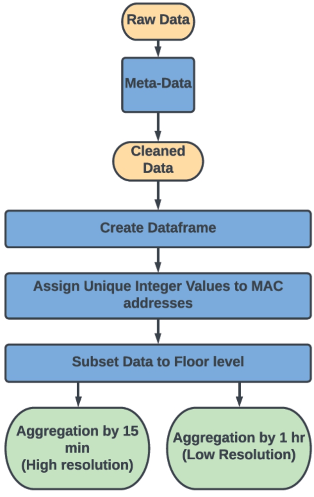
The available dataset does not explicitly provide the counts of devices, which are required for a time series forecasting problem. Hence, the counts need to be extracted using a data pre-processing step. The workflow for producing these counts is visualized in Fig. 1. First we obtain the meta-data by going through the raw data and understanding how the building is being utilized. This helps us identify redundant fields such as the month and more importantly helps us identify how the Access-Point field can be used to distinguish and filter the data by individual floors. We then use the meta-data to only select relevant information. In addition to this any Virtual Local Area Network (VLAN) entries were removed. This results in cleaned Data which contains Wi-Fi log entries with the date, time-stamp, MAC address, and corresponding AP fields. The cleaned data is used to create a DataFrame and each field is assigned its corresponding data type. Next, the MAC addresses were replaced by random integers (referred to as ID) to maintain the anonymity of the devices, and the data was sorted by time. Following this, the AP field was used to select entries for the first floor only. Finally, two key levels of aggregation over time intervals were selected as one hour and fifteen minutes. An hour is a standard measure for many activities, especially on campus. Over a large interval (such as an hour), the number of counts follows the assumption that all the users recorded stayed on the floor for the entire hour. To relax this assumption, a smaller 15-minute aggregation interval is proposed. We are also interested in capturing more microscopic level patterns, which is ensured by the 15-minute interval. The data obtained from 15-minute intervals was also less noisy compared to 5- or 10-minute intervals. For these reasons, the smaller aggregation interval of 15 minutes called High Resolution (HR) and a larger aggregation interval of 1-hour called Low Resolution was selected.
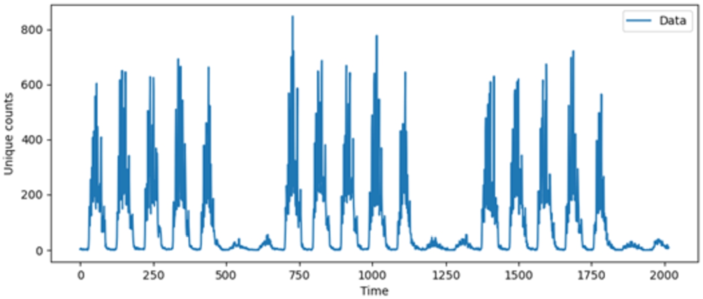
In the aggregation stage, the dataset was duplicated into two, one for each determined time interval (LR and HR). In each, the unique ID addresses were counted at their corresponding intervals. This results in the occupancy count datasets of LR and HR where each consists of a single field of counts at their corresponding intervals of aggregation. There are 2016 samples in the HR dataset and 504 samples in the LR dataset. Figure 2 displays the counts plot observed over three weeks for the high-resolution dataset.
Each dataset is further split into training and testing datasets, where the train data were used to develop the model and the test data used to evaluate the model. A data split of 67% and 33% was used for training and testing, respectively. This choice was made to provide ample data to the models to learn underlying patterns and at the same time perform testing on a full week to observe day-specific performance.
Fig. 2.
High Resolution (HR) data.
4.2.Autoregressive Integrated Moving Average (ARIMA)
ARIMA models are popular for time-series prediction problems and serve as the base case for comparison in our work. The basic Autoregression and Moving Average (ARMA) model requires that the time series to be modelled should be stationary. This means that there should be no trends or seasonality in the data. Therefore, ARMA models cannot be used for non-stationary data. We can remove any trends by employing differencing between the series until it results in stationary data, which exhibits behaviour similar to white-noise. This combination of autoregression (AR) and Moving Average (MA) models, which include differencing, is known as ARIMA. Equation (1) shows how the current value in the series is related to past differenced values of the series. Here,
The optimal ARIMA models are obtained for LR and HR datasets. The model parameters p and q were initialized to the values obtained by interpreting the autocorrelation (ACF) plot and the partial autocorrelation (PACF) plots followed by iterative improvements [21]. Walk forward validation is also applied when testing the ARIMA models, which means that we re-train the model whenever new data becomes available. This is appropriate for our time-series problem because as we keep testing our model, we expect new information to become available, which we can use to re-train the model for better predictive ability.
4.3.Multi-layer Perceptron (MLP)
MLP is a feedforward artificial neural network (ANN) with an input and an output layer. It can have any number of intermediate (or hidden) layers as described by the researcher. Information is propagated through layers, and the model learns by adjusting the weights of the neurons through backpropagation. The neurons are parts of the layers, which form a linear combination of the weights W and inputs x with an added bias term b as shown in (2). The output of the neurons is passed through an activation function ϕ, and the result is propagated through the network. The adjustable parameters of the MLP are the number of neurons, the number of layers, number of epochs, batch size, and the activation function.
The performance of the MLP depends on how well the hyper-parameters are tuned for the given problem. We also introduce a walk-forward validation in the MLP model. Additionally, the model is repeated ten times, and the average RMSE is reported along with the standard deviation in RMSE. This is done to address the stochastic nature of the algorithm, where different predictions are obtained each time the model is evaluated. Repeating and reporting the standard deviation of the error in RMSE also serves as an evaluation metric because a good model will result in small deviations for repeated trials. The mean squared error is used as the loss function with the Adam optimizer.
4.4.Long Short-Term Memory (LSTM)
This work is focused on developing an LSTM framework and evaluate it against the other baseline models. Since occupancy prediction varies across time, we can expect correlations between various timesteps. Recurrent Neural Networks (RNN) are a special ANN that addresses these time dependant correlations. However, one drawback of RNN is that they encounter the exploding or vanishing gradient problem, which prevents them from capturing long-term time dependencies. LSTM is a special form of RNN that uses memory cells and three gates to overcome the problems in RNN [6,8]. Each memory cell makes the prediction
The performance of the LSTM also depends on how well the hyper-parameters are tuned for the given problem. Therefore, various hyperparameters are tuned, which include the number of neurons, number of layers, and lookback period (which is how many previous time steps are used to make a prediction). The mean squared error is used as the loss function with the Adam optimizer. Batch normalization between LSTM layers and Dropout layers serves as regularizes in the model to avoid overfitting to the training set. The stated hyperparameters were iteratively adjusted to improve the LSTM model performance.
LSTM models are implemented in this study are strategically developed. First a single layer LSTM is trained and evaluated on the LR data. The aim is to observe if the simpler LR dataset patterns can be learned by the basic LSTM cells. If this is true then the single layer LSTM is trained on the HR dataset. When it is found that the LSTM cannot adequately learn the patterns, additional layers of LSTM are introduced and evaluated.
4.5.Auxiliary LSTM (Aux-LSTM)
The LSTM methodology described in the previous section considers various complexities in its architecture, however, they are all univariate models. It is a form of sequential modelling where previous occupancy is used to predict future occupancy. This structure allows us to judge the robustness of the LSTM in forecasting using limited information, however, it doesn’t consider the applicability, especially in the context of facilities management and optimization. When we consider the operations perspective of this case study, we have limited control variables. To address this we focus on deriving additional information from the counts and couple it with the best LSTM configuration. We refer to this additional information as Auxiliary variables.
One key variable that can be derived from the counts is the flow. Flow of occupancy can be defined as the rate at which occupancy changes at a point. Flow variable can be very useful in the facilities management, as it can be controlled by the manager of the building or campus. This can mathematically be viewed as the derivative of counts
We obtain the Auxiliary variable only for the HR dataset so that we can see its effects at the microscopic level. After obtaining the auxiliary variable, we have to incorporate it into the LSTM. In this study we look at two ways of doing this, which results in two distinct Auxiliary LSTM architectures. The first method is to use the auxiliary variable as an input variable to the LSTM along with the Data Counts, this is called the ‘Observed Auxiliary Architecture’ or O-Aux-LSTM visualized in Fig. 3. By combining the two input features we end up with a multivariate LSTM structure for this case only.
Fig. 3.
Observed auxiliary architecture.
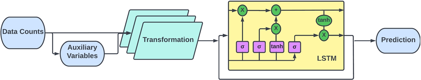
Fig. 4.
Joint auxiliary architecture.
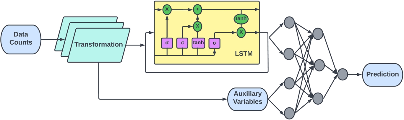
The second method is to only use Data Counts as input to the LSTM, then use the Output of the LSTM along with the Auxiliary variables to train a DNN which predicts future occupancy. This is refereed to as ‘ Joint Auxiliary Architecture’ or J-Aux-LSTM shown in Fig. 4. Both architectures provide a unique way of coupling Auxiliary information with standard LSTM. This will provide insights to whether the auxiliary information is significant as a primary input or as supplemental information. Finally, the Auxiliary variable highlights the importance of Wi-Fi dataset as a rich and flexible source. The Aux-LSTM were repeated ten times, and the closest average RMSE and
4.6.Limitations
The limitations of using Wi-Fi log data include overestimation of users due to multiple devices owned by a single user and underestimation due to users not connected to the network. A design choice in our methodology is that the selected study area has uniform activities taking place (i.e., classrooms); hence this model may not be accurate for heterogeneous activity spaces (such as offices or cafeterias), which makes it less transferable. It is also important to state that the stochastic nature of ANN models required hyper-parameter tuning, which was time-consuming because of the many parameters that need to be optimized. One limitation to the models was that the available data had unique patterns for peak hours, by using more data to train the same models we can expect higher accuracy in results.
The underestimation and overestimation of Wi-Fi can be addressed by adjusting the Wi-Fi counts using a strategically placed sensors and deploying methods used in studies [5]. To enable the transferability of LSTM, the study area can be expanded to include other types of activity spaces. Then the dominant activity taking place in a space can be inferred and used as a feature in the model. On the issue of feature engineering, the day of the week can also be used as an input feature in future indoor mobility studies. With additional input features in aux-LSTM, SHAP analysis can be used to understand the role and significance of each input. Since machine learning based models are black-box models we cannot fully interpret them. The proposed methodology in this study to select models and their parameters was through a logical approach as they are the variables we can control. Alternatively, this study can be conducted in a way where optimization algorithms are used to tweak the model parameters. SHAP analysis can then be used to help in interpretation of the model. Another dimension that can be explored is that the LSTM can be modelled on the log-differenced data similar to ARIMA, which may improve model performance. With a larger dataset, seasonal trends in the data can also be modelled.
4.7.Evaluation
The
Due to the complexity of the modelling procedures, it can be difficult to summarize model performance using a single statistic. We also provide fit plots that visualize how well the predicted counts reflect the true counts. We also take into account the prediction of peak and low values. Modelling the peak values correctly is especially important because under-predicting high occupancy can have more severe effects than under-predicting low occupancy. For example, in a resource allocation scenario, under-predicting can mean many individuals will not be accommodated during peak hours if such a model was used in the decision-making process. We selected the optimal lookback based on a balance between the highest performance and the lowest number of lookback periods possible so that large sequences of past information are not required for predictions.
5.Analysis and results
For data preparation and feature extraction, Python language is used. The MLP and LSTM were also implemented in Python using Keras library [4] and its implementation of TensorFlow [1]. ARIMA was implemented using the statsmodels [19] module in Python.
5.1.ARIMA
The nature of the data is time-series, and the observations depend on the time they are observed. This means that the time series is non-stationary and needs to be addressed before modelling. The Augmented Dickey-Fuller (ADF) test is a unit root test used to test the null hypothesis that the time series is non-stationary [21]. For both datasets (LR and HR), the null hypothesis was accepted for a significance level of 0.05, concluding that both datasets are non-stationary. The scalloped shape of the ACF plot for original HR data indicates that there are trends in the data [9] as shown in Fig. 5.
Fig. 5.
ACF and PCF of original and transformed HR data.
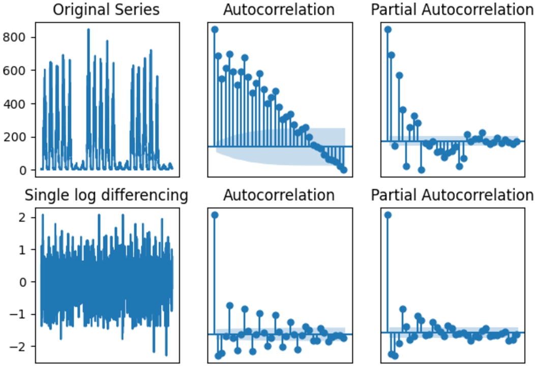
A log transformation was applied to the datasets to convert the time series into a stationary time series and remove the trend, followed by differencing. Single differencing was found to be the optimal level in both datasets. Performing the ADF test on each of the transformed series concluded that the resulting series are stationary. Hence the degree of differencing d in the ARIMA model was set to 1. The PACF and ACF plot in Fig. 5 for both LR and HR data were used to obtain initial values for ARIMA followed by iterative improvements. The optimal configuration of ARIMA(p, d, q) for LR and HR datasets was (1,1,0) and (3,1,3), respectively.
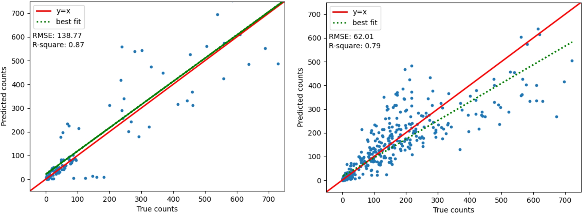
The fit plot for both datasets is shown in Fig. 6. The ARIMA model slightly overpredicted the LR data for smaller counts with an RMSE of 138.77 and heavily underpredicted the HR data with an RMSE of 62.01. In the density plots of both ARIMA models, LR and HR, the residuals resembled a leptokurtic distribution with a non-zero mean value which indicates there is bias in our model.
Fig. 6.
(a) Left: LR ARIMA fit-plot. (b) Right: HR ARIMA fit-plot.
5.2.MLP
The MLP model configurations are defined as the number of inputs (n1), the number of hidden layer neurons (n2), epoch (e), and batch-size (b). First, we outline the results with walk-forward validation. The best MLP model configuration on LR data was (5, 20, 30, 1) with an average RMSE of 97.86 and a standard deviation of 4.78. The closest results to the mean statistics from the ten repeats in LR are shown in Fig. 7(a), and its corresponding
Now we outline the results of MLP without walk forward validation, repeated ten times. The LR data (10, 40, 21, 1) had an RMSE of 87.39 with a standard deviation of 8.70. The HR data (10, 50, 50, 100) had an RMSE of 49.30 with a standard deviation of 1.01. The MLP models with and without walk forward validation predicted peak values slightly well, but the model without walk forward validation predicted lower values poorly, with significant negative value predictions. For this reason, the models with walk forward validation were selected as the best models.
Fig. 7.
(a) Left: LR MLP fit-plot. (b) Right: HR MLP fit-plot.
5.3.LSTM
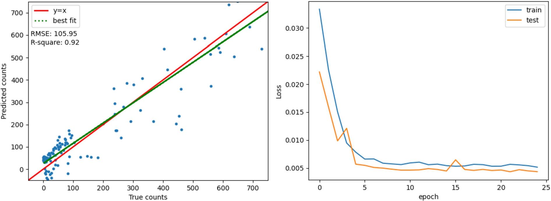
The first LSTM, called LSTM1, is implemented on the LR dataset had a single layer with five lookback periods and 20 neurons. It resulted in an RMSE of 105.95 and an
Fig. 8.
(a) Left: LSTM1 fit-plot. (b) Right: LSTM1 bias-variance plot.
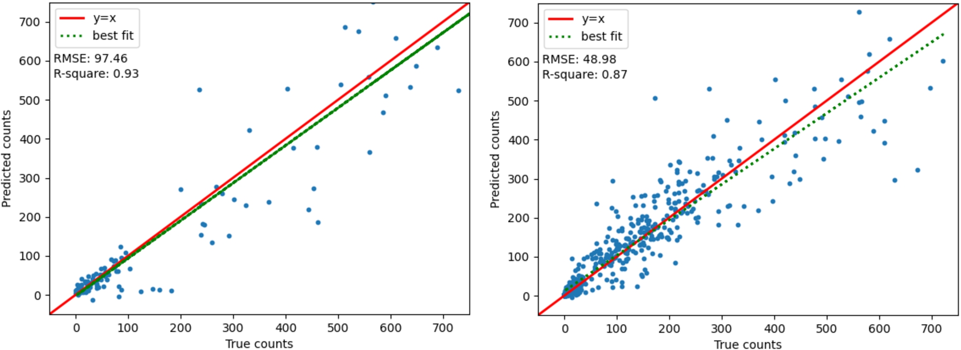
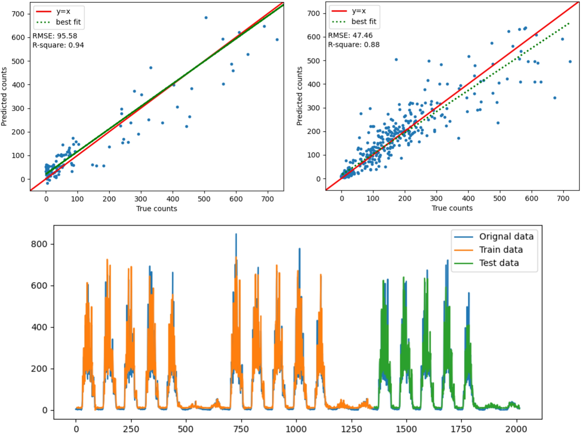
The second model, LSTM2, is implemented with two LSTM layers on LR data. We outline the optimal configuration of LSTM as (n1, n2, e, b, l), which translates to neurons in the first layer, neurons in the second layer, epochs, batch size, lookback. After tuning the hyperparameters, LSTM2 was found to be better than LSTM1 at modelling occupancy peaks with an R-square value of 0.94. The LR LSTM had the configuration (60, 50, 100, 20, 10). One key observation while developing the model was that changing the neurons in the first LSTM layer impacted the lower occupancy levels and the second layer of the LSTM impacted the peak occupancy counts. Figure 9(a) shows the fit plot of LSTM2. The bias-variance plot showed that train and test variance converges, which indicates that there is no overfitting.
The model for HR data is developed in a similar manner and is labelled as LSTM3. Two LSTM layers with a configuration of (40, 30, 650, 100, 10) including the regularizers, were the best hyperparameters for LSTM3. The tight cluster of points for most counts around the y = x line in Fig. 9(b) also indicates that the model predictions are homogeneous with the true counts. Although there is increasing variation for larger occupancy counts, we can get an understanding of the scale of variation in peak values by comparing the average RMSE of 40.6 to the largest observation of counts on the test set (a value of 721 peak occupants). The ratio is approximately 5.6%, which can be considered an acceptable level of variance. A visualization of predicted values to the original data is provided in Fig. 9(c), which visualizes how well LSTM3 captures peak occupancy.
Fig. 9.
From top left: (a) LSTM2 fit-plot. (b) LSTM3 fit-plot. (c) LSTM3 predictions overlay on data.
5.4.Auxiliary LSTM (Aux-LSTM)
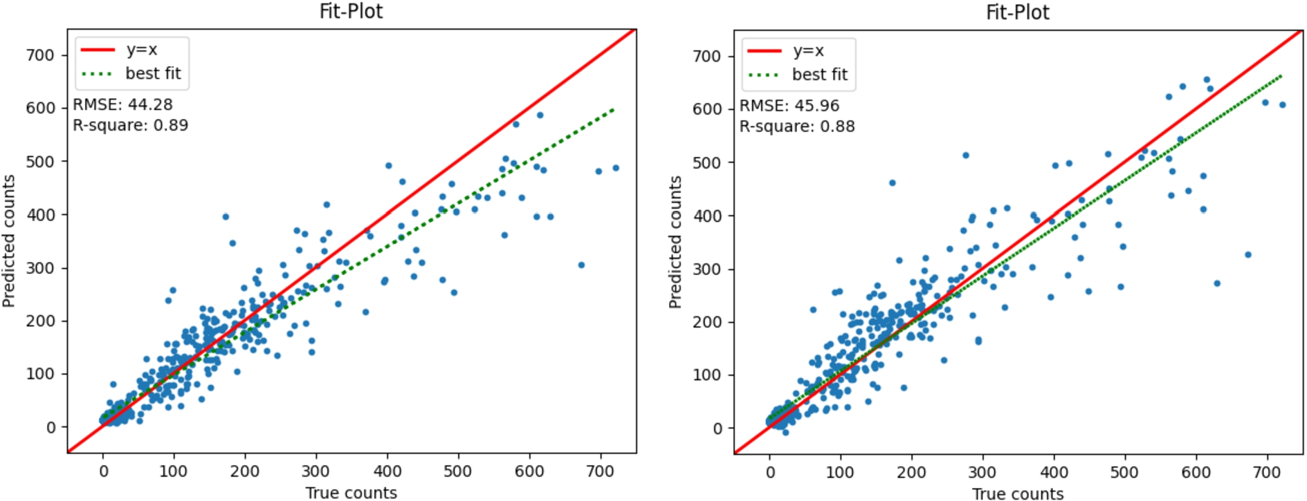
The best LSTM from the previous section was LSTM3 with hyperparamaters (40, 30, 650, 100, 10) and two layers. This configuration was used for both Aux-LSTM with HR data counts. Both O-Aux-LSTM and J-Aux-LSTM converged and there was no evidence of overfitting in their bias-variance plots. The average RMSE of O-Aux-LSTM was 44.3 with an
Fig. 10.
From left: (a) O-Aux-LSTM. (b) J-Aux-LSTM.
5.5.Comparative analysis
In all models, the RMSE observed was greater for the LR dataset. This can be due to the large fluctuation in peak occupancy counts of HR, which skew the RMSE towards lower values. All models were able to capture the daily trends in the data. More specifically, all models were able to predict higher volumes on weekdays and increasing occupancy till midday then declining afterwards.
The conical deviation observed for peak values in the HR ARIMA fit plot can be due to difficulty in modelling the rapidly changing occupancy counts shown in Fig. 2. The MLP model had the same pattern in performance in both datasets, where the lower values are predicted much better than the peak values. Overall, the MLP over-predicted the occupancy. Compared to ARIMA, the MLP has a more uniform deviation of true versus predicted counts. This highlights the significance of having a relaxed functional form in DNN models. The LR LSTM (LSTM3) fit-plot in Fig. 9(a) performed the best in terms of RMSE,
Each day in the HR dataset had a unique pattern for the peak values on weekdays, and a reason for the varying peak value trends is the area of the study itself. Campus occupancy does not have a regular day to day pattern such as that in offices because the peak values observed are a function of the number of classes taking place on any specified day. This proved to be challenging for the models to capture. This can be overcome by using long term data to train the models so that underlying patterns and seasonality in the data can be captured more effectively.
The best model on HR data was LSTM. As observed in Fig. 9, the LSTM mirrors the peak values well. The largest deviation observed is on day 4 of week 2 (orange train data prediction); however, this deviation is justified because that day exhibits a new pattern that was unobserved earlier. Hence the LSTM was not able to model it. From this, we can conclude that if trained for enough weeks, the LSTM can be a powerful tool for occupancy prediction in complex environments where collecting and accounting for details (such as class schedules) can be challenging. The occupancy prediction capacity of LSTM on HR data also shows that it is possible to model large volume of occupants, which has been a concern in studies [10]. As seen in Fig. 9 there are well over 600 occupants at floor-level during peak hours and LSTM is reasonably able to predict the counts.
Fig. 11.
Box-plot of repeated RMSE.
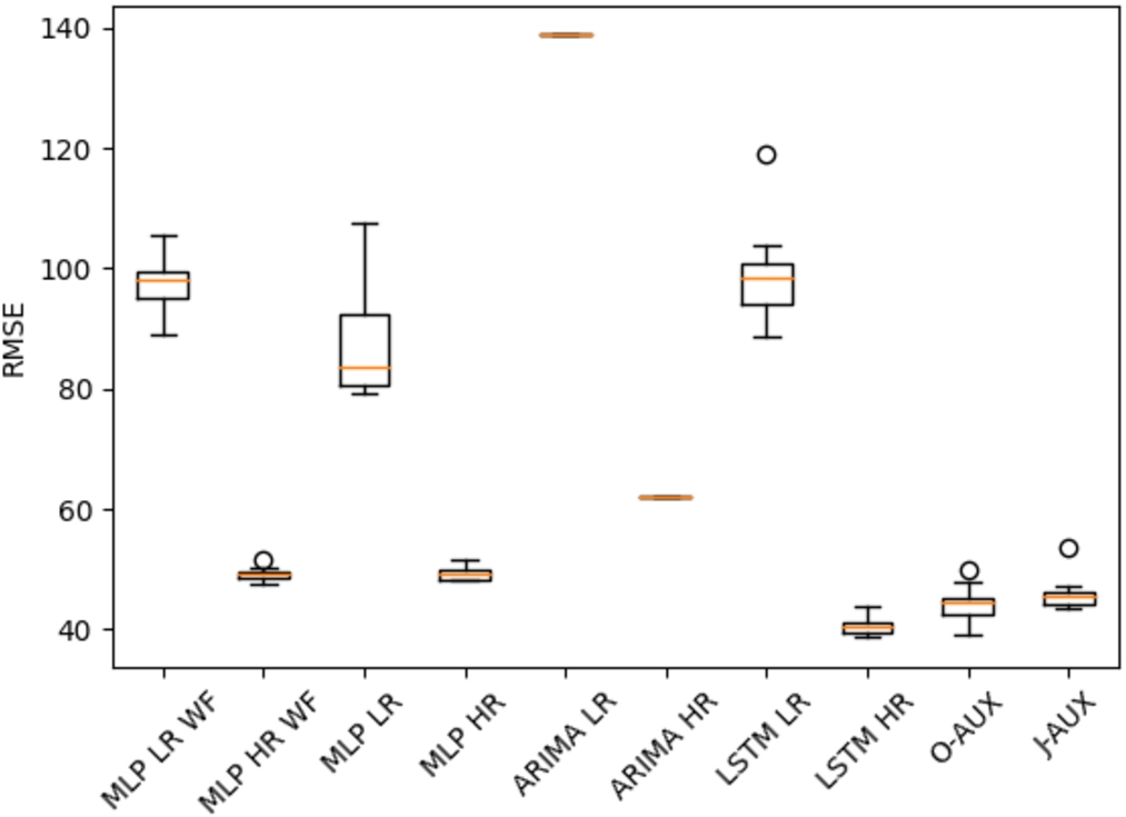
The box plots for RMSE of models are shown in Fig. 11. ARIMA does not show any variation because it is not repeated. LSTM performed the best on high-resolution data with a 17% better average RMSE compared to the second-best MLP model. An improvement from [25] is that our best LSTM model (LSTM2) performs well at modelling peak values. Peak occupancy predictions are only 5.6% inaccurate which can be considered acceptable at floor level.
Amongst the LSTM and Aux-LSTM models, LSTM performed slightly better in terms of RMSE. However, the Aux-LSTM still performed significantly well compared to other models. The difference between LSTM HR and O-Aux is 8%, and the difference between LSTM HR and J-Aux is 12%. These minor differences should not be considered only at face value. It should be noted that the fit-plots for each LSTM indicate large difference between true and predicted value for peak occupancy, which can skew the results. Furthermore, the frequency of large occupancy values is much lower than small occupancy values. Thus the effect of the difference of RMSE between the models is within acceptable bounds.
The availability of data also limits all models in their predictive capacity. This is more true for advanced models such as LSTM and Aux-LSTM which learn patterns in the data. The full data consisted of three weeks where two weeks were used in training and one week was used in testing. It should be noted that each week had a significantly different pattern especially during peak hours. This can be identified as a reason for LSTM and Aux-LSTM models to struggle in predicting peak occupancy.
By observing the Box-plot in Fig. 11, we observe that O-Aux has a higher variance than LSTM HR. This provides us the insight that using auxiliary variable as an input is not contributing useful information to the LSTM. When comparing LSTM HR to J-Aux we can see there is reduction in accuracy. However, the variance of RMSE is much less in J-Aux. The smaller variance translates to a higher reliability in prediction which can be a suitable trade-off in applications of facility management.
By introducing the auxiliary variable, we loose a very small amount of accuracy of the model. However, we gain access to another control variable (i.e., flow) which is a parameter that can be used by decision makers and facility managers to improve operations or simulation based digital twin.
Walk forward validation was shown to improve the MLP models. If data collection, data processing, and model fitting can be automated, allowing for real-time operation, then using walk-forward validation can allow the use of simpler models depending on the use-case.
6.Discussion and conclusions
Occupancy prediction can be used in many applications such as operational decision-making, facility management, and can even be used as a feature space to develop other models. The use of ubiquitous networks has the potential to be used due to their large-scale application and low cost. We propose a methodology for inferring occupancy counts using Wi-Fi log data. The flexibility in processing the Wi-Fi data allows us to study various aggregation levels that can be used to interpret the data for different use cases. The aggregation of data over time intervals shows us that Wi-Fi data can accurately capture daily trends over time. By building sequences of time steps, the data is formulated for a time series prediction problem. LSTM was found to be superior to other models in capturing high-resolution data. We can also extract valuable information from Wi-Fi data such as flow which can be used as auxiliary variables. We use Wi-Fi data to derive auxiliary variable and implement it in two architectures of LSTM. It was found that using auxiliary variable and LSTM output, connected through a DNN, we can increase reliability of results with negligible loss of accuracy, while making the model more useful for the facilities manager and decision makers. For example, a more reliable model can be used in HVAC control. The accurate and high resolution models can be used in simulation studies. By using high resolution models, it is also possible to reduce their predictions to low level through aggregating the occupancy counts over the required time interval. This provides a temporal resolution for planners, designers, and makes this methodology integratable with digital twins. Our methodology provides a bottom-up approach to tackle occupancy prediction, where we model floor-level occupancy that can be expanded to building and campus level occupancy. An alternative method is to use a top-down approach where data of buildings with similar attributes can be aggregated and a generalized building level model can be created. Similarly, floor level data with same attributes can be aggregated and a generalized floor level model can be created. This can perhaps also overcome the limitation of requiring long term data as many different patterns can be learnt from various buildings with similar attributes.
Acknowledgements
This research is supported by Smart Campus Digital Twin, a Natural Science and Engineering Council’s Alliance project with FuseForward.
Conflict of interest
None to report.
References
[1] | M. Abadi, P. Barham, J. Chen, Z. Chen, A. Davis, J. Dean, M. Devin, S. Ghemawat, G. Irving, M. Isard et al., Tensorflow: A system for large-scale machine learning, in: 12th {USENIX} Symposium on Operating Systems Design and Implementation ({OSDI} 16), (2016) , pp. 265–283. |
[2] | L. Alfaseeh, R. Tu, B. Farooq and M. Hatzopoulou, Greenhouse gas emission prediction on road network using deep sequence learning, Transportation Research Part D: Transport and Environment 88: ((2020) ), 102593. doi:10.1016/j.trd.2020.102593. |
[3] | J.C. Augusto (ed.), Handbook of Smart Cities, Springer International Publishing, Cham. ISBN 9783030696979; 3030696979. |
[4] | F. Chollet et al., Keras, GitHub, 2015, https://github.com/fchollet/keras. |
[5] | B. Farooq, A. Beaulieu, M. Ragab and V.D. Ba, Ubiquitous monitoring of pedestrian dynamics: Exploring wireless ad hoc network of multi-sensor technologies, in: 2015 IEEE Sensors, IEEE, (2015) , pp. 1–4. |
[6] | S. Hochreiter and J. Schmidhuber, Long short-term memory, Neural computation 9: (8) ((1997) ), 1735–1780. doi:10.1162/neco.1997.9.8.1735. |
[7] | W.-C. Hong, Application of seasonal SVR with chaotic immune algorithm in traffic flow forecasting, Neural Computing and Applications 21: (3) ((2012) ), 583–593. doi:10.1007/s00521-010-0456-7. |
[8] | Y. Hua, Z. Zhao, R. Li, X. Chen, Z. Liu and H. Zhang, Deep learning with long short-term memory for time series prediction, IEEE Communications Magazine 57: (6) ((2019) ), 114–119. doi:10.1109/MCOM.2019.1800155. |
[9] | R.J. Hyndman and G. Athanasopoulos, Forecasting: Principles and Practice, OTexts, (2018) . |
[10] | W. Jung and F. Jazizadeh, Human-in-the-loop HVAC operations: A quantitative review on occupancy, comfort, and energy-efficiency dimensions, Applied Energy 239: ((2019) ), 1471–1508, https://www.sciencedirect.com/science/article/pii/S030626191930073X. doi:10.1016/j.apenergy.2019.01.070. |
[11] | A. Kalatian and B. Farooq, Mobility mode detection using WiFi signals, in: 2018 IEEE International Smart Cities Conference (ISC2), (2018) , pp. 1–7. doi:10.1109/ISC2.2018.8656903. |
[12] | A. Kalatian and B. Farooq, A semi-supervised deep residual network for mode detection in Wi-Fi signals, Journal of Big Data Analytics in Transportation 2: (2) ((2020) ), 167–180. doi:10.1007/s42421-020-00022-z. |
[13] | S. Kim, Y. Sung, Y. Sung and D. Seo, Development of a consecutive occupancy estimation framework for improving the energy demand prediction performance of building energy modeling tools, Energies 12: (3) ((2019) ), 433. doi:10.3390/en12030433. |
[14] | X. Li, G. Pan, Z. Wu, G. Qi, S. Li, D. Zhang, W. Zhang and Z. Wang, Prediction of urban human mobility using large-scale taxi traces and its applications, Frontiers of Computer Science 6: (1) ((2012) ), 111–121. |
[15] | M.S. Mirnaghi and F. Haghighat, Fault detection and diagnosis of large-scale HVAC systems in buildings using data-driven methods: A comprehensive review, Energy and Buildings 229: ((2020) ), 110492. doi:10.1016/j.enbuild.2020.110492. |
[16] | Z. Patterson and K. Fitzsimmons, DataMobile: Smartphone travel survey experiment, Transportation Research Record 2594: (1) ((2016) ), 35–43. doi:10.3141/2594-07. |
[17] | G. Poucin, B. Farooq and Z. Patterson, Activity patterns mining in Wi-Fi access point logs, Computers, Environment and Urban Systems 67: ((2018) ), 55–67. doi:10.1016/j.compenvurbsys.2017.09.004. |
[18] | M. Rezaie, Z. Patterson, J.Y. Yu and A. Yazdizadeh, Semi-supervised travel mode detection from smartphone data, in: 2017 International Smart Cities Conference (ISC2), (2017) , pp. 1–8. doi:10.1109/ISC2.2017.8090800. |
[19] | S. Seabold and J. Perktold, Statsmodels: Econometric and statistical modeling with python, in: 9th Python in Science Conference, (2010) . |
[20] | M.A. Shafique and E. Hato, Use of acceleration data for transportation mode prediction, Transportation 42: (1) ((2015) ), 163–188. doi:10.1007/s11116-014-9541-6. |
[21] | R.H. Shumway, D.S. Stoffer and D.S. Stoffer, Time Series Analysis and Its Applications, Vol. 3: , Springer, (2000) . |
[22] | H. Song, R. Srinivasan, T. Sookoor and S. Jeschke, Smart Cities: Foundations, Principles, and Applications, John Wiley & Sons, (2017) . |
[23] | M.W. Traunmueller, N. Johnson, A. Malik and C.E. Kontokosta, Digital footprints: Using WiFi probe and locational data to analyze human mobility trajectories in cities, Computers, Environment and Urban Systems 72: ((2018) ), 4–12. doi:10.1016/j.compenvurbsys.2018.07.006. |
[24] | T.M. University, Campus Master Plan, Technical Report, 2019. |
[25] | Z. Wang, T. Hong, M.A. Piette and M. Pritoni, Inferring occupant counts from Wi-Fi data in buildings through machine learning, Building and Environment 158: ((2019) ), 281–294. doi:10.1016/j.buildenv.2019.05.015. |
[26] | A. Yazdizadeh, Z. Patterson and B. Farooq, Ensemble convolutional neural networks for mode inference in smartphone travel survey, IEEE Transactions on Intelligent Transportation Systems 21: (6) ((2019) ), 2232–2239. doi:10.1109/TITS.2019.2918923. |
[27] | H. Zhang and L. Dai, Mobility prediction: A survey on state-of-the-art schemes and future applications, IEEE Access 7: ((2018) ), 802–822. doi:10.1109/ACCESS.2018.2885821. |
[28] | Z. Zhao, W. Chen, X. Wu, P.C. Chen and J. Liu, LSTM network: A deep learning approach for short-term traffic forecast, IET Intelligent Transport Systems 11: (2) ((2017) ), 68–75. doi:10.1049/iet-its.2016.0208. |
[29] | Y. Zheng, Q. Li, Y. Chen, X. Xie and W.-Y. Ma, Understanding mobility based on GPS data, in: Proceedings of the 10th International Conference on Ubiquitous Computing, (2008) , pp. 312–321. doi:10.1145/1409635.1409677. |
[30] | H. Zou, Y. Zhou, H. Jiang, S.-C. Chien, L. Xie and C.J. Spanos, WinLight: A WiFi-based occupancy-driven lighting control system for smart building, Energy and Buildings 158: ((2018) ), 924–938, https://www.sciencedirect.com/science/article/pii/S0378778817313907. doi:10.1016/j.enbuild.2017.09.001. |


