
McStas (ii): An overview of components, their use, and advice for user contributions
Abstract
A key element of the success of McStas is the component layer where users and developers alike are contributing to the description of new physical models and features. In McStas, components realise all physical elements of the simulated instrument from source via optics and samples to detector. In this second review paper of the McStas package, we present an overview of the component classes in McStas: sources, monitors, optics, samples, misc, and contrib. Within each component class we give thorough examples of high-quality components, including their algorithms and example use. We present two example instruments, one for a continuous source and one for a time-of-flight source, that together demonstrate the use of the main component classes. Finally, we give tips and instructions that will allow the reader to write good components and elucidate the pathway of contributing new components to McStas.
1.Introduction
We present the second article in a review series concerning the neutron simulation package McStas. The first article in the series described the package, its use, philosophy, and mathematical background [29]. For reasons of clarity and conciseness, we will here often refer to material in the previous article.
Since the foundation of McStas in 1997–1998 the software has been Open Source and Free Software.11 From the start, it has been our vision that our users – often instrument scientists at neutron facilities or expert neutron users at universities – should be able to work from a set of basic ready-made elements. In addition, the users should be able to easily contribute new functionality to the software by means of new sections of code [15]. This basic philosophy led to McStas having a strongly modular structure, where individual optical elements were programmed in separate files, known simply as components, whereas a full neutron scattering instrument was described in so-called instrument files, that made use of (a subset of) the programmed components. The components may realise all physical elements of the instruments to be simulated, from source via optics and samples to detector(s).
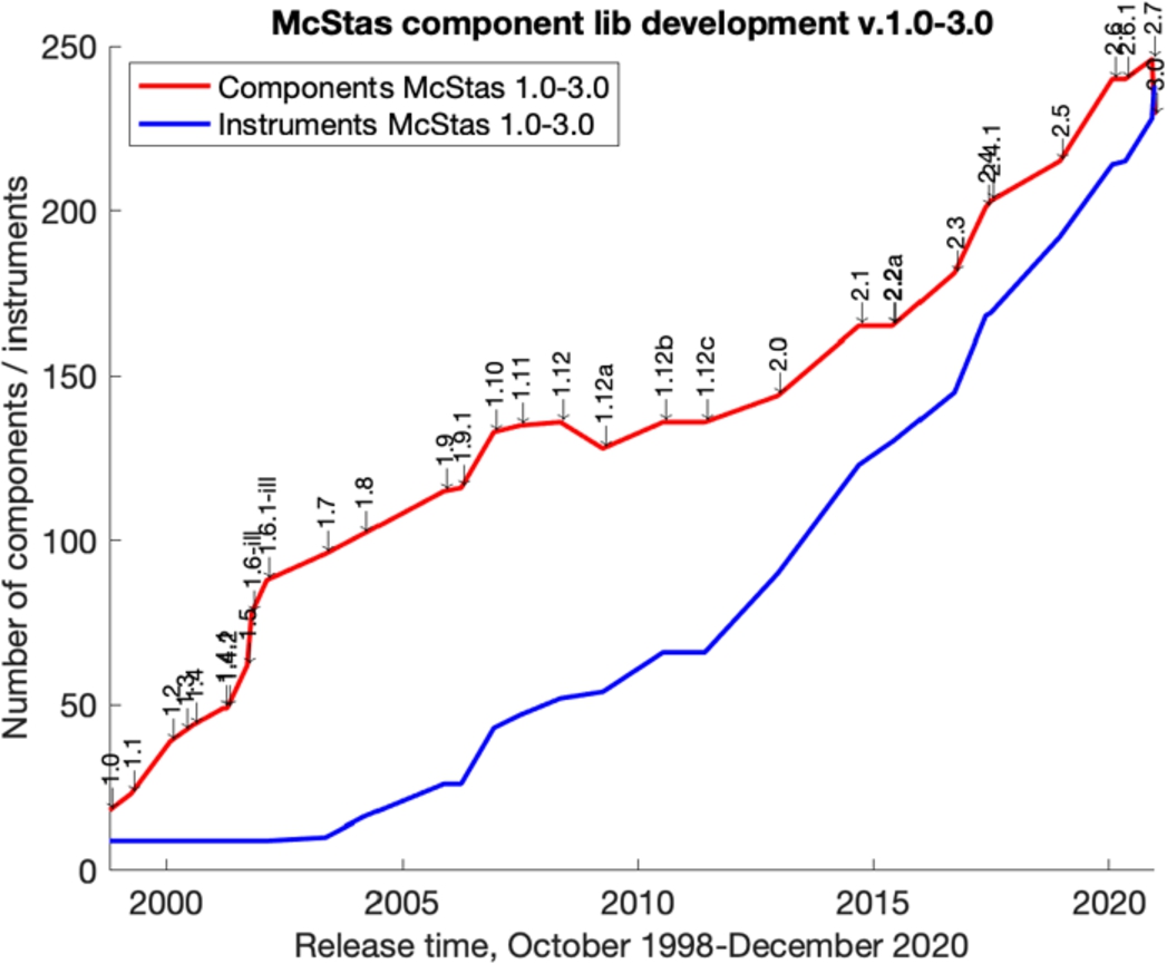
By this separation of instrument-near functionality from the (complex) basic McStas system, it has proved possible for users and the central McStas team alike to develop a large number of components, each with a different purpose. In most cases, each component contains less than 200 lines of C-code, facilitating overview and maintenance by persons different from the author. Since year 2000, the component library including the example instrument files has been the largest growth area of the McStas project, as illustrated in Fig. 1.
In this article, we will present the different classes of McStas components and present selected components in additional detail. We will present two demonstration instrument files that contain most of the selected components: A two-axis diffractometer for a continuous source and a powder diffractometer for a time-of-flight source. In addition, we will elaborate on the expectations for component contribution to the McStas project, with the hope that this will inspire even more user contributions in the future.
Fig. 1.
The development of the number of components in the McStas component library since the beginning of the project….
2.The McStas component categories
The McStas component library is naturally divided into categories, depending on the component functionality. The categories in the current (v. 2.6) release are:
Sources: | Components used to define the starting condition of the neutron state. In McStas the term source corresponds to the neutron moderators of real-world facilities like steady-state reactor sources or pulsed spallation sources. The reason for this is that McStas does not include the needed physics to describe e.g. fission or spallation.22 In McStas we also provide sources of a purely mathematical nature, e.g. a (non-)divergent source and a point source. |
Monitors: | To measure or visualise beam characteristics in the instrument, McStas includes so-called monitor components. Almost all monitors can be said to be perfect probes of the neutron state, i.e. no physical detection process is simulated. The output of a monitor generally is a one- or two-dimensional histogram, but can also be a list of neutron events. |
Optics: | This component category covers any device on the instrument used to transport or manipulate the neutron beam. Examples are super-mirror neutron guides, slits and collimators, rotating optics like disk choppers or velocity selectors or Bragg optics like monochromators.33 |
Samples: | Components used to model matter on the beam-line, e.g. to be included as a scientific sample in an experiment. Since this review series will include a dedicated article on these complex components, the paper at hand only includes a brief overview of the available models. |
Misc: | Components that do not fit in the other categories. Examples are the components supporting i/o for the MCPL particle list format and the Scatter_logger components used to study beam-losses in neutron guide systems. |
Contrib: | Components that are written by McStas users (i.e. not the package developers). This is a rich library of functionality for McStas in categories of sources, monitors, optics and samples. A special case among these components are the contrib/Union components written by Mads Bertelsen [3], allowing to assemple complex arrangements of material and perform multiple scattering within this assembly, e.g. a sample inside a cryostat. |
2.1.Component basics
A McStas component receives an incoming neutron state (a ray) (x,y,z,vx,vy,vz,t,sx,sy,sz,p)in from the McStas system, then transports, records or manipulates the state and finally returns the resulting neutron state (x,y,z,vx,vy,vz,t,sx,sy,sz,p)out back to the McStas system.
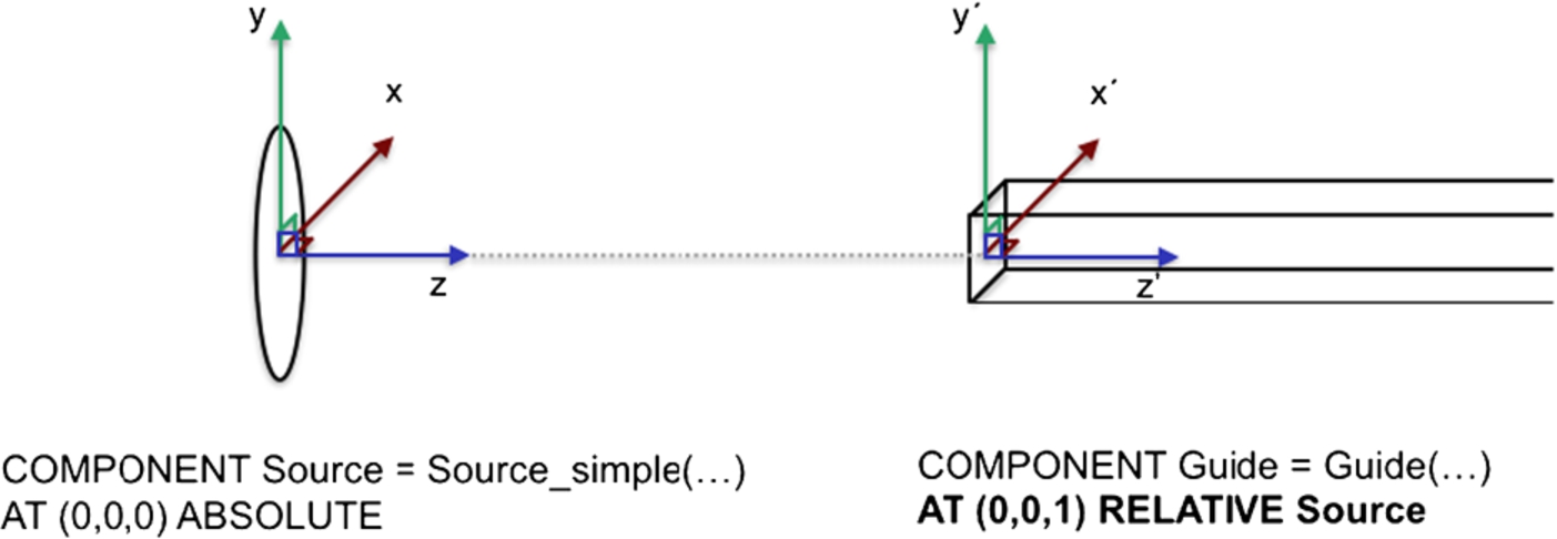
The component coordinate system can be chosen freely as to whatever is the easy system of the device/problem at hand. However, the usual starting condition in McStas sources is to have z along the neutron beam and y vertical, and since our coordinate system is right-handed x is horizontally transverse to the neutron beam, pointing left as seen from the source. This convention is then naturally carried over to other components in the instrument, e.g. a neutron guide would typically be translated along z seen from the source, as shown in Fig. 2.
Fig. 2.
(top) Illustration of a neutron source (left) and the entrance of the primary guide (right), displaced 1 m along the positive z direction. (bottom) the McStas instrument file code corresponding to the source and the primary guide.
2.2.Component structure
To be a valid McStas component, a file needs to be written in the syntax of the C-language and have the following structure and properties
Filename If our intended component is a Foobar, a good filename would be Foobar.comp
Documentation header The first section in the component file is a documentation header, enclosed in c-style (/*…*/) comments. This section contains subsections
%I – Information about who wrote the component, when and where
%D – Description of what exactly Foobar is and how it is supposed to be used, usually with an example use of Foobar in an instrument context, i.e. Example: Foobar(Par=3.1416)
%P – Parameter list of format:
∗ Par: [unit] Description of Par
%L – Optional subsection, typically with scientific references or hyperlinks
%E – marks the End of the document header
DEFINE COMPONENT Foobar Declares that the component is a Foobar (label should match the chosen filename).
DEFINITION PARAMETERS () List of component input ‘define’ parameters, i.e. given to the component in the form of a c-style #define compiler directive. Was historically used to enable allow lists, pointers and other base types not supported by the SETTING PARAMETERS list below. Support for this type of parameter has been removed in McStas 3.0 and instead the vector type has been added, see next paragraph.
SETTING PARAMETERS () List of parameters for the component. Type can be double (default if no type is explicitly given), int, string and in McStas 3.0 also the vector class, initialised by a (static) {1,2,3} type array or through an instrument variable defined via DECLARE and INITIALIZE sections in the instrument.
OUTPUT PARAMETERS () List of (internal) variables in the component that should be made private, i.e. masked from the scope of other components of the same type present in the instrument. (What technically happens is a variable-prefixing based on the component instance name.) The OUTPUT PARAMETERS are ignored in McStas 3.0, as all component parameters automatically become members of a named struct for the given component instance.
SHARE %{ … %} Section to define common types (e.g. structs) and functions for all used components of type Foobar. Hence included only once in the generated c-code.
DECLARE %{ … %} Section to declare variables of the component. In the McStas 3.0 release, this section is used to automatically generate a component struct, so please avoid initialization with explicit values, such as double a=1.0; .
INITIALIZE %{ … %} Section to initialize (internal) variables and state of the component, based on the given input PARAMETERS. This is the place to do your sanity checks and put warnings / errors, potentially raising an exit(); if fatal.
TRACE %{ … %} This is where to write lines of C-code that control the action, i.e. handle your incoming neutron state (x,y,z,vx,vy,vz,t,sx,sy,sz,p)in, propagate, perform checks on the given neutron and perform calculations, and assign new values to variables in the state vector. Please consider using RESTORE_NEUTRON(INDEX_CURRENT_COMP,x,y,z,vx,vy,vz,t,sx,sy,sz,p) if your component could, after all, not do anything useful with the given neutron ray. This makes life easier e.g. in GROUPs of components acting in parallel.
MCDISPLAY %{ … %} This is where you draw a sketch of the component using a subset of these basic macros:
∗ line(x0,y0,z0,x1,y1,z1)
to draw a line between two points.
∗ dashed_line(x0,y0,z0,x1,y1,z1)
to draw a dashed line with n dashes between two points.
∗ multiline(n,x0,y0,z0,…,xn-1,yn-1,zn-1)
to draw a set of n line segments
∗ circle("xy",cx,cy,cz,radius)
draws a circle with given radius on the "xy" plane, centered at c. Give "xz" or "yz" to access the other component planes.
∗ rectangle("yz",cx,cy,cz,zwidth,yheight)
draws a rectangle of given dimensions on the "yz" plane, centered at c. Give "xy" or "xz" to access the other component planes.
∗ box(cx,cy,cz,xwidth,yheight,zdepth)
draws a box centered on a given point in space.
∗ cylinder(cx,cy,cz,r,h,N,nx,ny,nz,)
draws a cylinder centered on point c, directed along normal n with radius r, height h and with N lines to illustrate the cylinder wall.
∗ sphere(cx,cy,cz,r,N,nx,ny,nz,)
draws a sphere of radius r centered on c, with N lines illustrating longitude and latitude.
END Marks the end of the component code.
3.Example components from the library
We here attempt the difficult task of describing the contents of the McStas component library. For brevity, we limit ourselves to only a few examples within each component category. A description of all components can be found in the online component documentation on the McStas home page [21] and in the McStas component manual [22]. Two test instruments, showing the use of most components described, are presented in Section 4.
3.1.Sources
All McStas simulations start with a Source-type component, which can initialize the parameters of the simulated neutron ray, i.e. its position
In the first McStas review article [29], we presented the rule for intensities of a simulation at component j in the instrument,
This focusing was also discussed in Ref. [29], where we presented the fundamental equation
This is the initial weight used in the most basic source components, including the component Source_simple(), which is the one used in the first instrument example.
Different continuous sources can be provided in the same way, where only the flux function
For pulsed sources, there is a further complication that the intensity varies with time. The component Moderator() is a simple example of this. Here, the emission time is chosen from an exponential distribution,
A much more elaborate time-of-flight component is ESS_butterfly(), which covers the most recent description of the moderators for the European Spallation Source (ESS). An in-depth treatment of this component is out of the scope of this review, and we refer instead to the online documentation [21].
When a McStas component description or parameter-file does not yet exist for your source, an option is to use the MCPL_input component which makes use of the MCPL [9] framework. MCPL provides a very nice interchange-format for particle lists, with backends available for McStas and McXtrace, SIMRES [18]-[19], Vitess [30], Geant4 [1], PHITS [20] and several variants of MCNP [27]. Thus you can perform your McStas simulations with particle data directly out of your neutron source simulations performed in e.g. MCNP. You should however bear in mind that your derived McStas simulation is in principle statistically limited to what the chosen input-file contains and avioding bias can be dificult. The MCPL_input component provides facilities for smoothing when repeating the particle data an integer number of times, which e.g. happens implicitly when running MPI-parallel simulations. This is done by making Monte Carlo choices within a small sphere of confusion around each event in the input file. When using these user-parameters to resample the MCPL data, please examine your MCPL data carefully and make conservative choices, e.g. based on inspection of the particle distributions. Please also consider the energy-ranges available in your MCPL-input and set relevant, physically meaningful E_min and E_max limits in MCPL_input. – McStas is for instance not suited for transport of eV, keV, or MeV range neutrons!
3.2.Monitors
The term “monitor” in McStas is rather loosely defined and describes any way to gather information about the beam passing a component (typically a specified surface). The neutron ray is propagated until it intersects the specified surface, and the monitor component will determine whether the ray is within the boundary of the monitor. If so, the neutron ray will be registered in a way particular for each monitor (see details below). The monitor will keep track of both number of rays,
Unlike a physical monitor or detector, the neutron ray is not affected by the monitor and may continue after the interaction. In fact, if the flag Restore_neutron is set to 1, the neutron ray is even propagated back to its position from before the interaction with the monitor, just to ensure that the monitor is transparent to the other parts of the simulation.
Monitors are as ubiquitous as source components, since this is the only way McStas simulations can produce results. Typically, each monitor will produce one data file for every simulation run. Monitor data are almost always histogrammed. The corresponding bins are either one-dimensional (for example in the L_monitor() and TOF_monitor() described below), or two-dimensional (such as the PSD_monitor() and Divergence_monitor() described below). The physical size, the binning range and the number of bins are taken as input parameters for all monitor components. Routines for formatting one- and two-dimensional data to file are present in the McStas library, to ensure uniformity in data formats.
A number of monitors exist that can perform rudimentary data treatment, for example by transforming time-of-flight and scattering angle into scattering vector, given proper information on the instrument geometry. The use of such components may speed up the design of full instruments, since simulated data are immediately in a human understandable format. However, a detailed description of these more complex monitors is outside the scope of this review.
Below, we describe in more detail some of the most used monitor components.
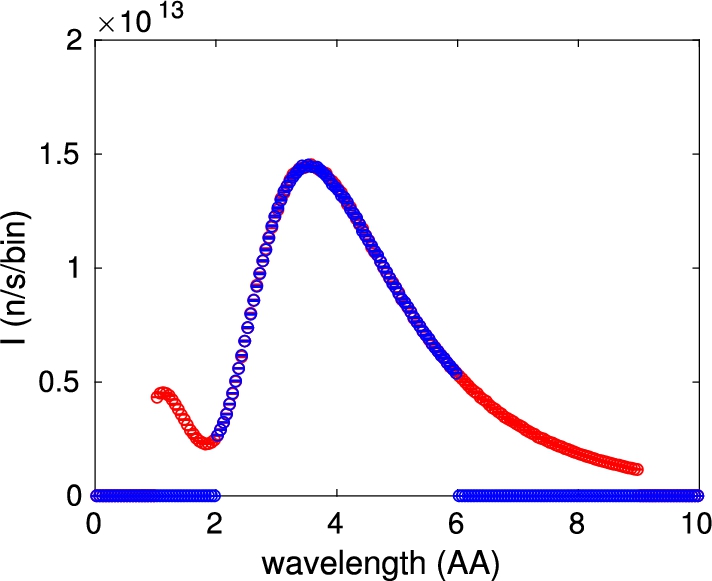
L_monitor(). This component is a rectangular shaped one-dimensional monitor that registers the true neutron wavelength and histograms the incoming intensity on a number of wavelength bins. A typical output from this monitor is shown in Fig. 3.
TOF_monitor(). This component is very reminescent of L_monitor(), only the neutron rays are distributed according to their arrival time at the detector surface. As such, it can be seen as a simple version of the physical time-of-flight detectors. A typical output from this monitor is shown in a later example, Fig. 9.
Fig. 3.
The simulation results obtained from shooting neutron rays from Source_Maxwell_3() into an L_Mon(), in effect showing the wavelength distribution of the source intensity. The Maxwellian source is run with two non-zero intensities, one corresponding to
PSD_monitor(). This monitor is another example that actually has a physical counterpart. It produces a two dimensional image of the neutron intensity in real space. It is often used to characterize the beam in a guide or just before the sample – or as the detector for neutron imaging instruments. An example of output from this component is shown in a later example, Fig. 7.
Divergence_monitor(). This two-dimensional monitor ditributes the neutrons according to their divergence in the two dimensions perpendicular to the detector normal. This unphysical monitor is usually used to inspect the phase space distribution of the beam inside a neutron guide system or at the sample position.
Monitor_nD(). This monitor can measure almost anything you can imagine, by means of a flexible options parameter string. Monitor_nD is very powerful, but using it correctly can take some effort and describing all features is out of the scope of this review. Instead, we refer to the relevant section of the McStas component manual, the Monitor_nD mcdoc page and the many McStas example instruments that make use of this component. The monitor can assume many geometrical shapes including flat panels, cylinders, spheres and a surface-description in OFF format, where each surface polygon becomes a pixel on the detector. The monitor generates 1-dimensional histograms (or multiples of these), 2-dimensional histograms and event lists with user-selectable columns of neutron data. This means that Monitor_nD can be used to measure anything the other monitors can do, and more. One powerful speciality is the use of the special user1,2,3 variables which can measure any c variable in your instrument file. An example of this can be found in the ILL_IN6 instrument by Emmanuel Farhi, found in the McStas examples: A variable measures which of the 7 IN6 monochromator blades has scattered the neutron, to be later correlated against the beam wavelength at the sample position. Further McStas-Mantid interface [17] to the Mantid [2] data reduction framework is implemented via a combination of mcdisplay.pl and Monitor_nD. Lastly, Monitor_nD can measure neutron states elsewhere upstream in your instrument file using the previous keyword or in combination with PreMonitor_nD (see below).
PreMonitor_nD(). The PreMonitor_nD component can store the neutron properties for use later in the simulation work flow, e.g. measure the originating state of the neutron at the source to be studied at the sample position. The component has a single input, namely the instance name of the Monitor_nD which will perform the measurement. (That Monitor_nD should correspondingly have premonitor in its options string.) The dedicated example instrument Test_PreMonitor_nD available in the McStas installation demonstrates its use.
3.3.Optics
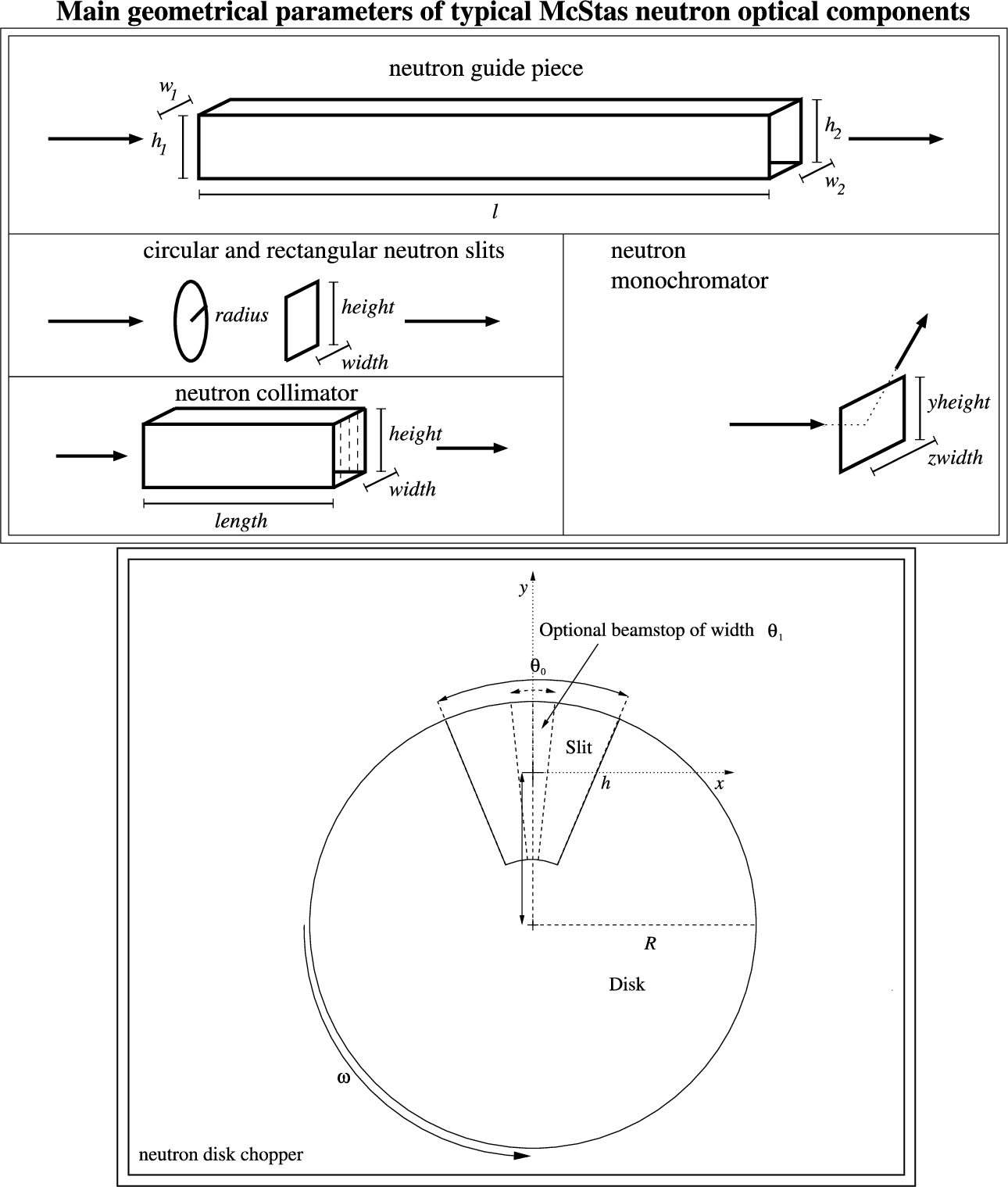
We now turn to the optical components that in general are used to modify the beam characteristics. The geometry of the components in this section is shown in Fig. 5.
Arm(). This is possibly the most used McStas component, yet it does not affect the neutron ray at all(!) The component is to be used as a reference for the internal coordinate system in McStas. Typically, an Arm() is placed at an axis of rotation, and following components – including further Arm()’s – are to be placed relative to the first Arm(). Used in this way, the Arm() component has the same function as an optical bench.
Slit() aka. Diaphragm(). This component is a simple slit, which in effect is an infinitely wide, 100% effective absorber with a single central opening, being either circular or rectangular. As rectangular, the slit opening width is given by the parameters xmin and xmax. Alternatively, a symmetric opening is given by instead setting the parameter xwidth. The corresponding parameters setting the opening height are denoted ymin and ymax, alternatively yheight. These variable names are generally used for heights and widths of components within McStas – as described in the (rarely studied) NOMENCLATURE document on the McStas home page [21].
If Slit() should rather have a circular opening (in this case centered at the origin of the local coordinate system), this is done by setting the input parameter radius. This way of controlling the component functionality via setting of input variables is a frequent feature within McStas library components.
The Slit() functions in the following way: First the neutron ray is propagated to the plane of the component. Next, a check is performed to see if the neutron has hit the slit opening. If not, the neutron ray is discarded, using the McStas command ABSORB.
Collimator_linear(). This component models a linear Soller collimator, physically made from a stack of absorbing, parallel blades. It is box-shaped with the physical dimensions xwidth, yheight, and length, as shown in Fig. 5. The degree of collimation is parametrised as the maximal divergence allowed through, using the parameters for the two directions: eta_x and eta_y – just as for a Soller collimators on an experimental set-up. If any of these parameters is zero, this is interpreted as if there is no collimation restriction in the corresponding direction (the default value).
The neutron ray is first propagated to the entry plane, then to the exit plane of the component. If the ray does not pass the collimator opening at both planes, it is ABSORB’ed. If the neutron ray has a larger divergence than the maximally allowed, in either the x or the y direction, it is also ABSORB’ed.
In a physical Soller collimator, the transmission of a certain neutron is either 0 or 1, depending whether the neutron trajectory intersects one of the absorbing plates. The test for collision for each of the plates is somewhat tedious, so in this McStas component we use a stochastic approach. If we assume that we do not know exactly where the absorber blades are positioned (but only the distance between them), we can calculate the probability of being transmitted as a function of divergence (for collimation in one dimension):
Guide(). McStas contains a number of neutron guide components. We here describe the simplest of them, Guide(). This is a neutron guide with rectangular openings. The entry has the dimensions h1 × w1, while the exit has dimensions h2 × w2, i.e. it is possible to describe a linearly tapering guide by making the entry and exit rectangles having different sizes. The length of the guide is given by l.
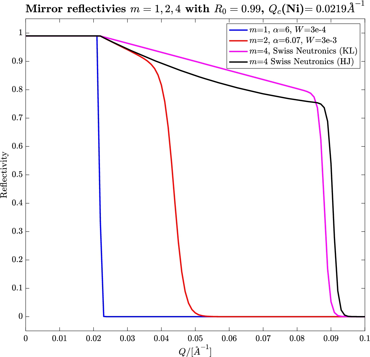
The inner surface of Guide() is imagined to be covered by a neutron-reflecting layer or layers, where the outermost layer is Ni, which has a critical scattering vector of
To quantify this, we need to define the actual scattering vector, q, in the conventional way,
The component functions by propagating the neutron ray to the entry plane. If the rectangular opening is not hit, the neutron is ABSORB’ed. Otherwise it continues into the guide. Each time the ray intersects one of the four guide sides, a specular reflectivity event is assumed. The scattering vector, q, is calculated, and the neutron weight multiplier becomes
For a consistent description of the mirror reflectivity, it can be recommended in stead of R0 and alpha to use the library ref-lib, which contains updated descriptions of reflectivity for mirrors of different values of m. This library is used for all McStas components that decribe optics with reflecting surfaces, such as Guide_gravity(), Guide_wavy(), Mirror() and several others. The current version of the reflectivity profiles is illustrated in Fig. 4.
Fig. 4.
The reflectivity profiles,
Monochromator_flat(). This component models a simple crystal monochromator of dimensions yheight × zwidth. The coordinate z is here used to denote the width, since the unrotated monochromator lies in the
The Monochromator_flat() is assumed to be an ideally imperfect mosaic crystal, i.e. it is assumed to have a Gaussian mosaic spread of tiny crystallites, each too small to have significant primary extinction. This, in turn, gives rise to a Gaussian distribution of the scattering from the monochromator. The divergence of the scattered beam is characterized by the parameters mosaich and mosaicv, for the horizontal and vertical directions, respectively. In other words, mosaich is the effective mosaic in the horisontal direction, such that an in-plane oriented monochromator will display a rocking curve width (FWHM) with the value mosaich. Likewise, mosaicv is the effective mosaic in the vertical direction, such that a pencil-beam reflected from the same monochromator will have a vertical spread (FWHM) of
Two other monochromators exist in the McStas package: Monochromator_curved() is a multi-slab composite of crystals, focusing the scattering to a particular point, while Monochromator_pol is a flat, neutron polarizing monochromator. Polarized neutrons are described in a later article in this review series.
Monochromators of perfect (or bent perfect) single crystals are at present not present in McStas, as primary extinction is not implemented. An approximation does however exist in the Single_crystal component, where the crystal lattice can be bent locally, keeping the external geometry of the crystal unchanged. In this approximation, curvature is spherical along the outer vertical and horizontal axes of the crystal.
DiskChopper(). This component models a disk chopper; a neutron-absorbing flywheel spinning with its axis along the beam direction, and with wedges cut into the wheel to let through neutrons at particular times. A sketch of the component is shown in Fig. 5.
The component takes the geometry parameters radius, nslit, yheight, theta0 – the latter representing the angular width of each slit (in degres). In addition, we have the chopper frequency nu (in Hz) and the phase of the choppers (at time zero), phase.
A special feature of this component is its effect on a continuous beam. Here, the intention is that the beam will be pulsed after hitting the chopper. However, naively used, this could result in a huge loss in simulated neutron rays. This we have remedied by letting all neutron rays pass the first chopper, while its time is being adjusted to a (random) value where the chopper was indeed open for this ray. This functionality is activated by setting the flag isfirst. It should, however, be used on the fist chopper only, since otherwise very misleading results could arise.
McStas also features other rotating optical components, such as the descriptions of spinning velocity selectors, Selector() and V_selector(), and two different descriptions of Fermi choppers, FermiChopper() and Vitess_ChopperFermi(). For descriptions of these components, we refer to the McStas documentation.
Fig. 5.
Geometries of the five described beam-optical elements with the standard naming of geometrical parameters shown. Top: Guide(), Monochromator(), Collimator() and Slit(). Bottom: DiskChopper().
3.4.Samples
At this place, we only briefly touch upon scattering samples in McStas, since a later article in this series is dedicated to exactly samples. For this reason, we here initially present two very simplified examples and then only list all presently available samples in McStas.
Incoherent(). This sample scatters all incoming neutron rays incoherently, i.e., uniformly in the
Powder1(). This sample introduces powder diffraction from a single value of q. The neutron rays are Bragg scattered out into different directions, forming a Debye-Scherrer cone. The scattering and absoption cross sections for the sample are parametrized by F2 and sigma_abs, respectively. The sample has a larger sibling, PowderN(), which can tackle an arbitrary number of powder lines, read from an specified crystallographic input file.
The McStas sample suite. For completeness, in Table 1 we list the presently available scatering samples in McStas. All samples take as parameters their physical size, their absorption (and possibly incoherent) cross section, and then a parametrized or file-based description of their scattering cross section.
Table 1
A list of sample components currently supported in the McStas package
| Component | Description | Comment | Reference |
| Incoherent | Simple incoherent scatterer | – | – |
| Tunneling_sample | Elastic and inelastic incoherent scatterer | – | [16] |
| Powder1 | Powder diffraction with 1 peak | – | – |
| PowderN | Realistic powder diffraction with N peaks | – | [28] |
| Single_crystal | A single crystal with multiple scattering | – | – |
| Sans_spheres | Small angle scattering from monodisperse spheres | – | – |
| SASView_model | A general SANS sample from the SASView library | – | – |
| Mirror | A sample with tabulated reflectivity | Also used as optical mirror | – |
| Phonon_simple | A simple acoustic-phonon sample on an fcc lattice | – | – |
| Isotropic_Sqw | A general inelastic powder sample | – | [6] |
| Magnon_bcc | A simple magnon sample on the bcc lattice | – | – |
| Res_sample | A “sample” used to calculate triple-axis resolution functions | – | [25] |
| TOFRes_sample | A “sample” used to calculate time-of-flight resolution functions | – | [25] |
3.5.Misc
Our miscellaneous component category contains the components that do not naturally fit into the other categories where physical properties are a common denominator, e.g. sources or samples. The most notable misc components are these:
Progress_bar(), does not interact with the beam, but monitors the ongoing simulation statistics. It prints output along the lines of Trace ETA 18 [s] % 57 60 70 80 90%. The flag_save parameter allows to trigger a save (i.e. write a set of intermediary files) when the simulation status is updated.
MCPL_input() and MCPL_output(), provide the McStas interface to the MCPL [9] framework. As also mentioned elsewhere, MCPL provides an easy-to-use interchange-format for particle lists, with support for McStas and McXtrace, SIMRES [18], Vitess [30], Geant4 [1], PHITS [20] and several variants of MCNP [27]. This means that you can use MCPL whenever you want to split your simulation in multiple parts, optionally simulated in different Monte Carlo softwares. We strongly recommend to use the MCPL components in place of Virtual_input() and Virtual_output() components, firstly since the binary MCPL files are more compact and secondly since nice tools are included for the handling (e.g. filtering or merging) and visualisation of the event list content.
Components for Scatter_logging, these allows to monitor where and how neutrons are scattered/reflected e.g. in a guide system. For further details, please consult the related publication [10] and the Test_Scatter_log_* instruments included with your McStas installation.
Shape(), allows to include a shape in your instrument for visualisation purposes (only). The component does not interact or scatter the beam in any way. Both simple geometries like spheres, boxes, cylinders or free-form OFF surface descriptions (via input files) are supported.
3.6.Contrib
The contrib component category is where a user-contributed component is placed for distribution with McStas. In principle we offer the same technical support for contributed components as the official components of the other categories, but the McStas authors did not write these component themselves and can therefore naturally not take full responsibility for their behaviour or performance. Yet, the contributed components are generally speaking both relevant and working as they should. There are currently 117 components in the contrib section, of different types. For author information, please consult the individual component definition.
Sources:
∗ ISIS_moderator and ViewModISIS are the legacy and new component implementations of the TS1 and TS2 target-stations at the ISIS facility in UK.
∗ SNS_source and SNS_source_analytic are components for modelling the SNS source at ORNL in Tennessee, USA.
∗ Source_gen4 is developed at PSI, Switzerland, derived from the Source_gen component, with addition of a high-energy tail describing special features of the SINQ spallation source at PSI. Source_multi_surfaces is also a PSI development and allows a ‘pixelated’ source with localised intensity and spectrum differences.
Optics:
∗ Many guides and benders:
∗ Guide_anyshape_r from TUM/MLZ, OFF-geometry guide allowing to specify reflectivity per surface element.
∗ Guide_four_side, Guide_four_side_2_shells, Guide_four_side_10_shells. Allows flexible-geometry definitions of guides with four-sided guides, optionally with semi-transparent walls. There are three versions of the guide type, each with 1, 2 and 10 layers of nested guide walls.
∗ Guide_honeycomb, can be used to model a guide with honeycomb geometry as seen e.g. in the ILL BRISP spectrometer.
∗ Guide_multichannel, multichannel neutron guide with semi-transparent blades. Allows to simulate bi-spectral extraction optics.
∗ Guide_curved, curved neutron guide.
∗ Guide_gravity_psd, guide-monitor hybrid that allows to monitor lost neutron intensity along the guide.
∗ Guide_m, similar to the usual Guide, but allows specification of reflectivity pr. surface.
∗ Vertical_Bender, a vertical bender that correctly takes gravity into account.
∗ Choppers: Two different Fermi choppers, FermiChopper_ILL and Fermi_chop2a. MultiDiskChopper a diskchopper that allows non-equidistant slits of varying size with just one component instance (with DiskChopper this must be done with a GROUP of components). StatisticalChopper chopper for describing a chopper with pseudostatistical pulsing as described in [26]. Vertical_T0a models a vertical-rotation-axis
∗ Collimators: Two different radial collimators, Collimator_ROC, an ideal radial oscillating collimator and Exact_radial_coll which is made of many trapezium shaped neutron-slits stacked radially.
∗ Filters and windows: Al_window, models Al-windows typically found at the ends of evacuated flight-tubes/guides. Filter_graphite and Saphire_Filter model graphite- and saphire neutron filters.
∗ Lenses: Lens and Lens_simple are two different implementations of refractive neutron lenses [8].
∗ Crystal monochromators/analyzers: Monochromator_2foc is a doubly-focusing monochromator, PerfectCrystal and Spherical_Backscattering_Analyser are two different implementations for backscattering analyzers.
∗ Slits and apertures: CavitiesIn and CavitiesOut together form a 2-dimensional set of input and output apertures. The multi_pipe component allowes to define a 2-dimensional grid of slits.
∗ Mirror_Elliptic models an elliptic mirror, Mirror_Parabolic models a parabolic mirror, Mirror_Curved_Bispectral Mirror_Elliptic_Bispectral are circular and elliptical mirrors intended for bispectral beam-extraction.
∗ Polarisation-oriented components: Foil_flipper_magnet models a TU Delft type [14] foil-flipper with an inclined, magnetised foil, Pol_bender_tapering models a tapered polarising bender, Pol_triafield models a triangular field for e.g. SEMSANS, He3_cell models a 3He cell, Pol_pi_2_rotator models a field-device to rotate the neutron beam polarisation by
Samples have been contributed in various scientific areas
∗ Single crystal models: Single_crystal_inelastic, elastic and inelastic scattering from a single crystal. Single_magnetic_crystal: magnetic diffraction from a single crystal.
∗ Single crystal/powder models: NCrystal_sample, elastic and inelastic scattering models from the NCrystal model framework [5]. NCrystal models elastic and ineleastic single crystals, powders and to some extent also liquids based on material scattering kernels.
∗ Powders/polyscrystalline: Sample_nxs, provides general powder/polycrystalline scattering with neutron-matter interaction based on neutron cross section calculations of a unit cell. SiC models scattering from nanocrystalline silicon-carbide.
∗ SANS: 16 contributions, 4 from FZ Jülich and 12 from the Niels Bohr Institute.
∗ Reflectometry: Multilayer_Sample that allows constructing a multilayer and performs dynamical scattering theory.
∗ Samples for studying resolution: Spot_sample defines discrete Dirac-δ functions in Q, ω.
Monitors: E_4PI is a spherical energy-monitor. NPI_tof_theta_monitor is a cylindrical ToF-angle monitor. NPI_tof_dhkl_detector is a cylindrical detector which converts time-of-flight data (x,y,z,time) to a 1D diffractogram in dhkl. PSD_monitor_4PI_spin measures parallel- and antiparallel spin-directions in a spherical geometry. Radial_div is a radial divergence sensitive monitor with wavelength restrictions. StatisticalChopper_Monitor is a monitor intended for combination with the StatisticalChopper component. PSD_Detector models an n times m pixel Position Sensitive Detector (PSD), box, cylinder or banana filled with a mixture of thermal-neutron converter gas and stopping gas. PSD_monitor_rad is a PSD monitor that allows for radial averaging, intended for SANS settings. SANSQMonitor is a circular detector measuring the radial average of intensity as a function of the momentum transform in the sample, intended for SANS settings. TOFSANSdet is a SANS detector for ToF-SANS.
Union: The union framework is an advanced tool to model complex arrangements of scattering materials, e.g. samples within complex sample environments. The author of union has recently become a full member of the McStas team, so these components will soon become promoted from the contrib section. Union contains features for scattering as well as monitoring the neutron beam, i.e. both sample-like and monitor-like functionality.
Shielding_logger: The shielding_logger components are a tool to estimate γ-production arising in and around neutron supermirror guides. The components correspond to a recently published model [11–13], and are implemented similarly to the so-called scatter-logger [10].
4.Two simple example instruments
We will here present two instruments created to exemplify (most of) the components highlighted in Section 3. For each instrument, we present the instrument, display the TRACE section of the instrument file, and show example output from the resulting simulations.
4.1.A two-axis diffractometer on a continuous source
Fig. 6.
The McStas instrument file describing a simple two-axis diffractometer on a continuous source.
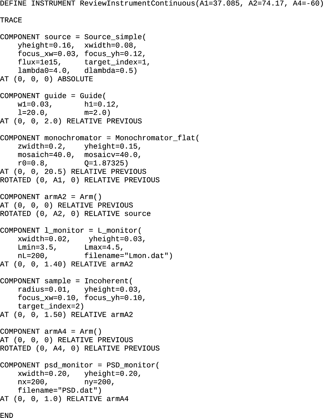
As the first example, we have assembled a very simple two-axis diffractometer on a continuous source, see Fig. 6. The instrument consists of a Source_simple() that feeds a neutron beam into a 20 m long,
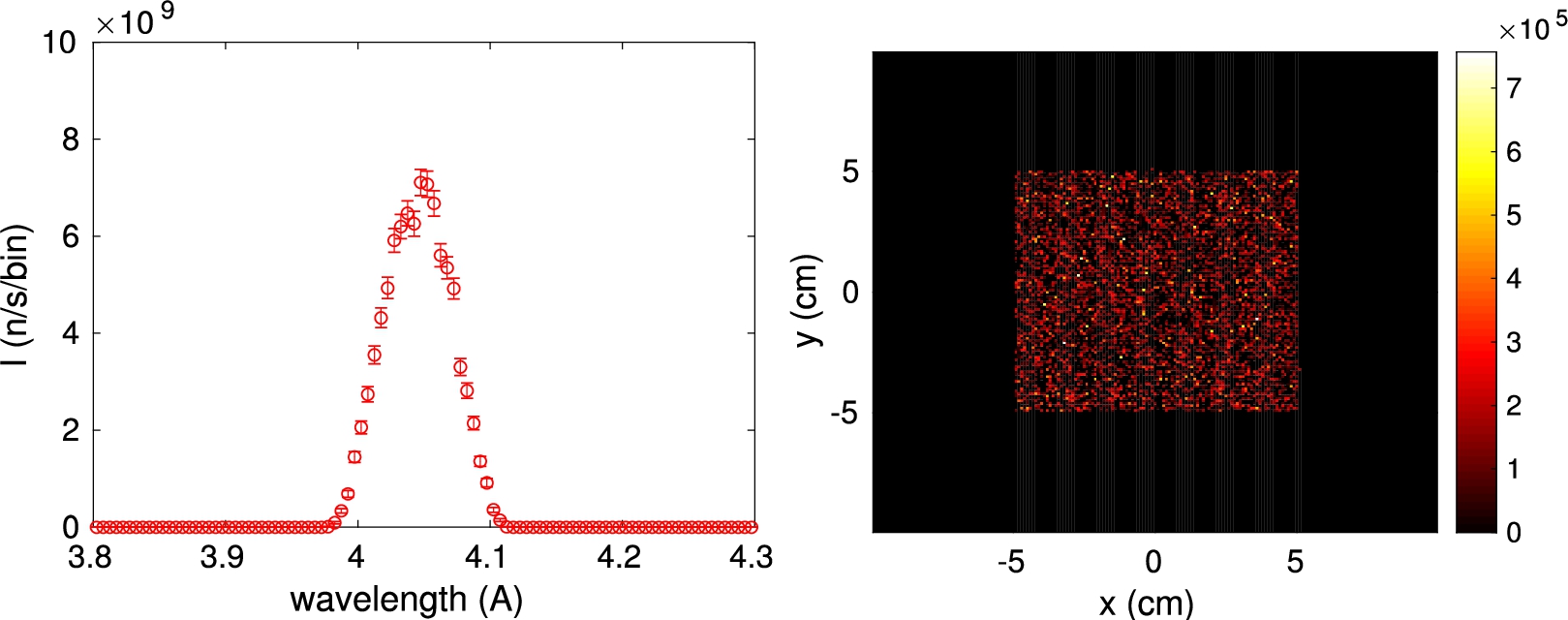
Typical results of simulations with this test instrument are shown in Fig. 7. The simulation is run with its default parameters: A2 value of 74.17° (corresponding to scattering of 5 meV neutrons on a PG monochromator), A1 being the half of this. Finally, we use as scattering angle, A4, a (somewhat arbitrary) value of 60°. The L_monitor shows a clear peak at
Fig. 7.
The simulation results obtained from the simple two-axis diffractometer in Fig. 6. (left) the wavelength distribution on the sample position as measured by L_monitor(). (right) The beam profile on the detector, measured by PSD_monitor().
4.2.A powder diffractometer on a pulsed source
The second example illustrates a very simple powder diffractometer at a pulsed source, as shown in Fig. 8. This instrument starts with a Progress_bar() that does nothing but generate information on the progress of the simulation. The neutron source is Moderator(), which is set to emit neutrons with energies between 2.5 meV and 6 meV. This is pulsed source, set to a pulse length of 100 μs. the neutron rays emitted from Moderator() are focused on a
After the source is placed a 50 Hz DiskChopper(), whose phase and opening angle can be controlled by external parameters, in this case PHASE and THETA. Next, the divergence of the beam is controlled by a Collimator_linear(), set to a maximum divergence of 60′ (60 arc minutes
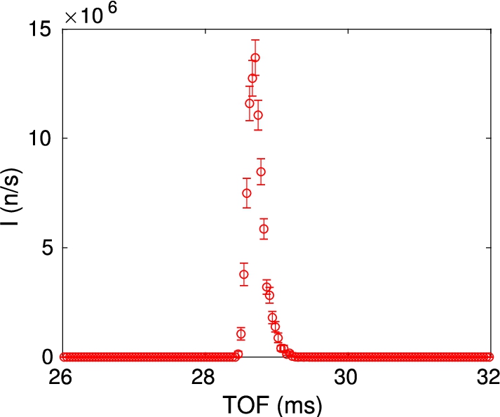
Figure 9 shows the outcome of this simple virtual experiment. A peak in intensity is seen close to a time of 28.7 ms. With a total flight path of
Fig. 8.
The McStas code for a simple powder diffractometer on a pulsed source.
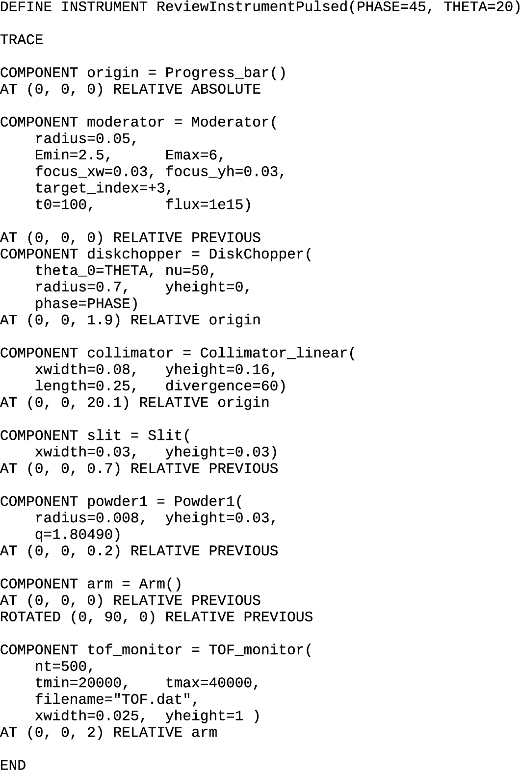
Fig. 9.
The simulation results obtained from the simple pulsed-neutron powder diffractometer in Fig. 8: the time dependence of the Braggdiffracted pulse on the detector position, as seen by a TOF_monitor().
5.Main elements of a good McStas component
For a component to become a user contribution in McStas, the list of formal requirements or ‘need-to-haves’ is relatively short:
(1) Have a correctly filled-in documentation header with full author information.
(2) Contain a readable and informative description of what the component can do.
(3) Have a well-described set of input parameters with physical dimension, preferably in “SI-units
(4) Describe how the given component differs from similar models already available in McStas.
(5) The component should further come with an example instrument, documented just as well as the component and demonstrating one or two typical settings and use-cases.
Where applicable, parameter names should be chosen in line with the McStas nomenclature description [24].
The component code has lots of explanatory comments for complicated or compact code, referencing relevant formulae from literature where needed.
Algorithms have generally been written aiming for clarity rather than having a complete physical description. For cases where accurate physical description is necessary, rather a dedicated component is written.
The related example instrument contains an %Example line, specifying what monitor output is expected in a test setting of the component.
Where applicable, the component has been tested in relevant asymptotic conditions, thereby reproducing either relevant theory or a given experimental condition.
6.The McStas review series
This article is the second in a series of McStas review papers. Planned themes in this series cover the main uses of McStas:
In addition to a review of these important cases, we also will describe a few topics of that deserve a more thorough and technical presentation than what has been given in literature so far:Modeling of scattering from samples
Simulation of polarized neutrons
Notes
1 McStas was originaly under a special RISØ license, but is since v.1.8 (2004) under GNU Public License v.2.0
2 To simulate such processes, multi-energy-multi-particle codes like e.g. MCNP [27], PHITS [20], FLUKA [4,7] or Geant4 [1] are needed.
3 Naturally, our diffracting sample components can also be used to monochromatize the neutron beam, but are most often also more demanding computationally, c.f. the Single_crystal component.
4 This paper.
Acknowledgements
It is a pleasure to thank everyone involved in the core McStas project over the decades. In chronological order: K. N. Clausen, K. Nielsen, H. M. Rønnow, E. Farhi, P.-O. Åstrand, K. Lieutenant, P. Christiansen, E. B. Knudsen, U. Filges, J. Garde, and M. Bertelsen.
References
[1] | J. Allison et al., Recent developments in Geant4, Nucl. Instrum. Meth. A 835: ((2016) ), 186–225. doi:10.1016/j.nima.2016.06.125. |
[2] | O. Arnold et al., Mantid–data analysis and visualization package for neutron scattering and μSR experiments, NIM A 764: ((2014) ), 156–166. doi:10.1016/j.nima.2014.07.029. |
[3] | M. Bertelsen, T. Guidi and K. Lefmann, McStas Union, (2021), in preparation. |
[4] | T.T. Böhlen, F. Cerutti, M.P.W. Chin, A. Fassò, A. Ferrari, P.G. Ortega, A. Mairani, P.R. Sala, G. Smirnov and V. Vlachoudis, The FLUKA code: Developments and challenges for high energy and medical applications, Nuclear Data Sheets 120: ((2014) ), 211–214. doi:10.1016/j.nds.2014.07.049. |
[5] | X.X. Cai and T. Kittelmann, NCrystal: A library for thermal neutron transport, Computer Physics Communications 246: ((2020) ), 106851. doi:10.1016/j.cpc.2019.07.015. |
[6] | E. Farhi, V. Hugouvieux, M.R. Johnson and W. Kob, Virtual experiments: Combining realistic neutron scattering instrument and sample simulations, J. Comp. Phys. 228: ((2009) ), 5251–5261. doi:10.1016/j.jcp.2009.04.006. |
[7] | A. Ferrari, P.R. Sala, A. Fasso and J. Ranft, “FLUKA: A multi-particle transport code” CERN-2005-10 (2005), INFN/TC_05/11, SLAC-R-773. |
[8] | H. Frielinghaus, J. Appl. Cryst. 42: ((2009) ), 681. |
[9] | T. Kittelmann et al., Monte Carlo particle lists: MCPL, Computer Physics Communications 218: ((2017) ), 17–42. doi:10.1016/j.cpc.2017.04.012. |
[10] | E.B. Knudsen, E.B. Klinkby and P.K. Willendrup, McStas event logger: Definition and applications, NIM A 738: ((2014) ), 20–24. doi:10.1016/j.nima.2013.11.071. |
[11] | R. Kolevatov, McStas and Scatter Logger driven calculations of prompt gamma shielding for neutron guides, Journal of Neutron Research 21: ((2019) ), 79–85. doi:10.3233/JNR-190123. |
[12] | R. Kolevatov, C. Schanzer and P. Böni, Neutron absorption in supermirror coatings, Journal of Neutron Research 20: ((2018) ), 127–129. doi:10.3233/JNR-180088. |
[13] | R. Kolevatov, C. Schanzer and P. Böni, Neutron absorption in supermirror coatings: Effects on shielding, NIM A 922: ((2019) ), 98–107. doi:10.1016/j.nima.2018.12.069. |
[14] | W.H. Kraan, J. Plomp, T.V. Krouglov, W.G. Bouwman and M.T. Rekveldt, Ferromagnetic foils as monochromatic π flippers for application in spin-echo SANS, Physica B: Condensed Matter 335: ((2003) ), 247–249. doi:10.1016/S0921-4526(03)00248-5. |
[15] | K. Lefmann and K. Nielsen, Neutron News 10: (3) ((1999) ), 20–23. doi:10.1080/10448639908233684. |
[16] | K. Lefmann, H. Schober and F. Mezei, Simulation of a multiple-wavelength time-of-flight neutron spectrometer for a long-pulsed spallation source, Meas. Sci. Techn. 19: ((2008) ), 034025. doi:10.1088/0957-0233/19/3/034025. |
[17] | T.R. Nielsen, A.J. Markvardsen and P. Willendrup, McStas and mantid integration, Journal of Neutron Research 18: ((2015) ), 79–92. doi:10.3233/JNR-160026. |
[18] | J. Saroun and J. Kulda, Physica B 234–236: ((1997) ), 1102. doi:10.1016/S0921-4526(97)00037-9. |
[19] | J. Saroun and J. Kulda, SPIE Proc. 5536: ((2004) ), 104; Saroun, J. and Kulda, J., SPIE Proc., 5536, 124, 2004. doi:10.1117/12.560925. |
[20] | T. Sato, Y. Iwamoto, S. Hashimoto, T. Ogawa, T. Furuta, S. Abe, T. Kai, P.E. Tsai, N. Matsuda, H. Iwase, N. Shigyo, L. Sihver and K. Niita, Features of particle and heavy ion transport code system PHITS version 3.02, J. Nucl. Sci. Technol. 55: ((2018) ), 684–690. doi:10.1080/00223131.2017.1419890. |
[21] | See the McStas home page at http://www.mcstas.org. |
[22] | See the McStas User Manual and the Component Manual at http://www.mcstas.org/documentation/manual/. |
[23] | The list of changes in McStas contains a summary of the most important changes in McStas for each release, It is published on the McStas website at http://mcstas.org/CHANGES_McStas. |
[24] | The McStas component nomenclature is defined in the file NOMENCLATURE found in your McStas installation and in the McStas GitHub repository https://github.com/McStasMcXtrace/McCode/blob/master/mcstas-comps/NOMENCLATURE.md. |
[25] | A. Vickery, L. Udby, N. Violini, J. Voigt, P.P. Deen and K. Lefmann, A Monte Carlo simulation of neutron instrument resolution functions, J. Phys. Soc. Jpn. 82: ((2013) ), SA037. doi:10.7566/JPSJS.82SA.SA037. |
[26] | R. Von Jan and R. Scherm, The statistical chopper for neutron time-of-flight spectroscopy, Nuclear Instruments and Methods 80: ((1970) ), 69–76. doi:10.1016/0029-554X(70)90299-5. |
[27] | S.C.J. Werner, J.S. Bull, C.J. Solomon et al., MCNP6.2 Release Notes, (2018) , LA-UR-18-20808, https://laws.lanl.gov/vhosts/mcnp.lanl.gov/pdf_files/la-ur-18-20808.pdf. |
[28] | P. Willendrup, U. Filges, L. Keller, E. Farhi and K. Lefmann, Validation of a realistic powder sample using data from DMC at PSI, Physica B 385–386: ((2006) ), 1032–1034. doi:10.1016/j.physb.2006.05.329. |
[29] | P.K. Willendrup and K. Lefmann, McStas (i): Introduction, use, and basic principles for ray-tracing simulations, Journal of Neutron Research 22: ((2020) ), 1–16. doi:10.3233/JNR-190108. |
[30] | G. Zsigmond, K. Lieutenant and F. Mezei, Neutron News 13: (4) ((2002) ), 11–14. doi:10.1080/10448630208218488. |


