Analysis of SESANS data by&nbsp;numerical&nbsp;Hankel transform implementation&nbsp;in&nbsp;SasView

Bakker, Jurrian H.; Washington, Adam L.; Parnell, Steven R.; van Well, Ad A.; Pappas, Catherine; Bouwman, Wim G.

doi:10.3233/JNR-200154

Analysis of SESANS data by numerical Hankel transform implementation in SasView

Article type: Research Article

Authors: Bakker, Jurrian H.^{a; *} | Washington, Adam L.^b | Parnell, Steven R.^a | van Well, Ad A.^a | Pappas, Catherine^a | Bouwman, Wim G.^a

Affiliations: [a] Radiation Science and Technology, Faculty of Applied Sciences, Delft University of Technology, Netherlands | [b] ISIS, Rutherford Appleton Laboratory, Chilton, Didcot, Oxfordshire, United Kingdom

Correspondence: [*] Corresponding author. E-mail: [email protected].

Keywords: Small-angle scattering, neutrons, SANS, SESANS, Hankel transform, SasView

DOI: 10.3233/JNR-200154

Journal: Journal of Neutron Research, vol. 22, no. 1, pp. 57-70, 2020

Published: 2 April 2020

Get PDF

Abstract

SESANS data analysis has been implemented in the SasView software package, allowing SESANS experiments to be analyzed using a numerical Hankel transformation of isotropic small-angle scattering (SAS) models. The error of the numerical approximation is three orders of magnitude below typical experimental errors. All advanced data fitting features of SasView (multi-model fitting, batch fitting, and simultaneous/constrained fitting) are now also available for SESANS and this is demonstrated by examples of fitting SAS models to SESANS measurements.

1.Introduction

Spin-Echo Small-Angle Neutron Scattering (SESANS) is a small-angle scattering technique for analyzing properties of condensed matter. It was first experimentally demonstrated by Keller et al. [13] and subsequently developed and made useful for analysis of real samples at the Delft University of Technology [6], where it has since been used to characterize many microscopic soft matter structures, such as colloidal suspensions [29], granular materials [1], food structures [31,33], and kinetics of structural changes [34]. The pioneering Delft SESANS instrument extends SANS to length scales reaching 20 μm and has inspired several other instrument development projects, such as a set-up using magnetic Wollaston prisms [19] and two time-of-flight instruments: Offspec [7,20,26] and Larmor [27], collaboratively developed by the Rutherford Appleton Laboratory and Delft University of Technology. Despite the successful design and implementation of these SESANS instruments, user-friendly data analysis tools have remained unavailable to a large extent. Here, we introduce the underlying theory of the numerical Hankel transform, and explain how it has been implemented into the SasView software package. We finally present several examples of successful data analysis, which highlight the capabilities of SESANS and the efficacy of the developed data analysis routines.

SESANS is a variant of the well-established Small-angle neutron scattering technique (SANS), which is itself a form of Small-angle scattering (SAS). The latter has been used over many decades to investigate properties of solids and liquids [10,11] and is a popular technique for material characterization. In a SANS experiment, a sample is placed in a beam of well-collimated neutrons and the small-angle scattering is detected by a position-sensitive detector. SESANS, on the other hand, uses the Larmor precession of polarized neutrons in carefully designed magnetic fields to label the scattering angle. The spin-echo principle can then be used to quantify this labelling to far smaller angles than a SANS instrument of comparable footprint and divergence could detect. Consequently, SESANS uses the available neutron flux far more efficiently than SANS at longer length scales. SESANS however, does not discriminate the scattered neutrons from the direct beam and thus works better in the presence of strong scattering, where multiple scattering corrections become important. Nonetheless, in contrast to SANS, these multiple scattering corrections can be easily accounted for in the SESANS data analysis [24]. Furthermore, the data interpretation is more accessible to non-experts in scattering techniques [4,5,12,22,24] for SESANS than it is for SANS. For the construction of an instrument with the combination of SANS and SEMSANS (Spin-Echo Modulated SANS) the reader is referred to the paper by Kusmin et al. [18].

SasView is an open-source software package for analyzing SAS experimental data written largely in the high-level programming language Python. It has a large, active community of developers from neutron and X-ray facilities and contains an extensive library of SAS model functions and fitting algorithms. As we will explain in the theory section below, for the analysis of the SESANS data the capabilities of SasView have been expanded to include the numerical Hankel transform, which is treated as a SAS resolution function.

2.Theory

In the following, we consider only small-angle scattering. In this case, the wave vector momentum transfer’s modulus Q is fully determined by the neutron wavelength λ and the scattering angle θ:

(1)Q=4πsin(θ)λ.

Furthermore, we will only consider radially homogeneous scattering, i.e. scattering with negligible azimuthal variation, such that the measured quantity of a SA(N)S experiment is the macroscopic differential scattering cross-section dΣ/dΩ. Without going into further detail, this function will be referred to as I(Q).

The measured quantity of a SESANS experiment is the polarization of the neutron beam P as a function of spin-echo length δ [1,13,17,22]. Spin-echo length is an experimental parameter that is determined by the neutron wavelength and the total magnetic field integral experienced by the neutrons. I(Q) and P(δ) are connected by the following equations:

(2)P(δ)=eλ2t(G(δ)−G(0)),

where t is the sample thickness and G(δ) is the “projected correlation function”, i.e. the 2D projection of the 3D auto-correlation function γ(r) [17], meaning that δ is the 2D projection of a radial distance r in 3D space. Alternatively, this can be re-written as the absolute scattering correlation function [16,24,35]:

(3)ln(P(δ))λ2t=G(δ)−G(0).

Assuming that all neutrons are detected [2],

(4)G(δ)=12π∫0∞I(Q)J0(Qδ)QdQ,

where J0 is the 0th order Bessel function of the 1st kind. In our SasView approach I(Q) is now a single-scatter SAS model function from the SasView library and G(δ) the SESANS fitting model. An example of I(Q) and J0(Qδ)Q on the same scale is given in Fig. 1. This means the left-hand side of Eq. (3) is entirely experimental and the right-hand side of Eq. (4) is entirely numerical. This separation is exploited to create the numerical Hankel transform (Eqs (6)–(22)). I(Q) can be defined by a single phenomenological function (SasView refers to such a function as a “shape-independent” function), or it can be defined as a combination of a form factor F(Q,x)2, a structure factor S(Q) and a parameter distribution PDF(x) (see Eq. (5)), which describes intra-scatterer interactions, inter-scatterer interactions and a distribution of SAS model parameters, respectively:

(5)I(Q)=S(Q)∫0∞F(Q,x)2·PDF(x)dx

where x can be one or several SAS model object parameters (e.g., the radius of a spherical colloid).

Fig. 1.

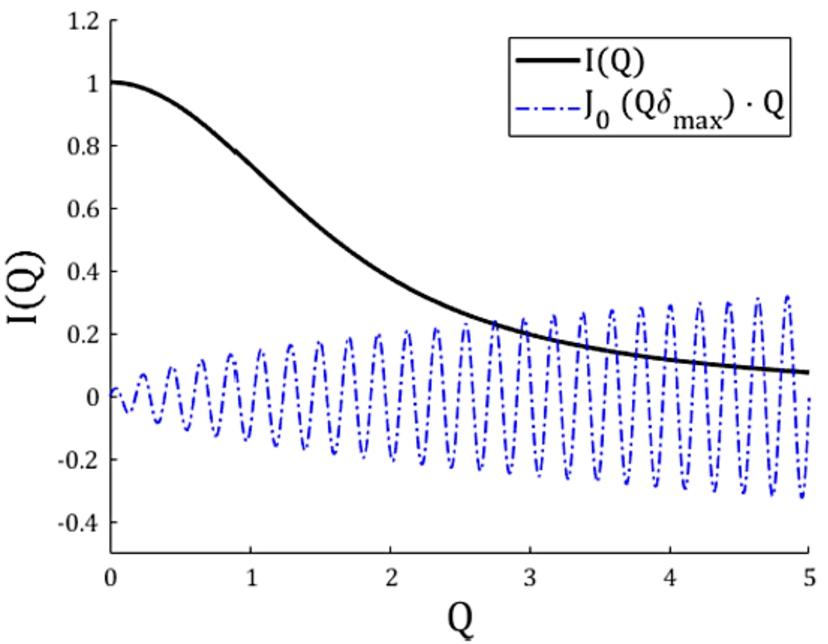
Plot of a scattering function I(Q), along with the zeroth order Bessel function of the first kind (J0) for δmax multiplied by Q. I(0) is assumed to be 1.

For our numerical approach, integrating Eq. (4) from zero to infinity is not possible. Therefore we must re-write this equation with lower and upper finite integration boundaries Qmin and Qmax. These are chosen such that the numerical errors of integration are negligible with respect to common SESANS experimental errors, which will be justified below:

(6)Gnum(δ)=12π∫QminQmaxI(Q)J0(Qδ)QdQ,

Gnum(δ)−Gnum(0) must approximate G(δ)−G(0) to minimize numerical errors. Furthermore, Qmax must be large enough to perform a full integration of (I(Q)×Q) for δ=0 and the step-size ΔQ must be small enough to sample J0(Qδ) for δ=δmax. This gives the following criteria:

(7)Qmax≫2πd,ΔQ≲2πδmax,

where d is the minimum characteristic length scale of the SAS model. Since every SAS model has a different d, this criterion is not practical. However, in practice, δmin≪d for all models and this can be used to create a robust criterion for Qmax. As the Q-space for the numerical integration is always linear in SasView, Qmin≡ΔQ. After testing, Qmax was judged to provide sufficient sampling without the need for scaling, while Qmin required scaling by a factor of 0.1. Taking these considerations into account, we arrive at the following criteria for the integration boundaries.

(8)Qmax⩾2πδmin,Qmin≡ΔQ⩽0.12πδmax.

At present, there is no option for the user to manually set the integration limits. The implementation of these mathematical formulations and conditions into SasView is as follows: firstly, δ, the spin-echo length, is a 1D array of size Z (taken directly from the experimental data) and Q is a 1D array of size N,

(9)δ=δ1δ2…δZ,(10)Q=Q1Q2…QN,

where the values of Q are determined by

(11)Qn=(0.1·2πZ·(δZ−δ1))·n;n∈{1,2,…,N}

and N is determined from the cut-off value Qmax: QN⩽Qmax.

(12)Qmax=2πδ1,

J0(Qδ) is the outer product of Q and δ with the 0th order Bessel function of the 1st kind J0 applied to all elements and is a 2D array of size [N,Z]. Since N scales with Z2, this array, and all subsequent arrays based on it, scale as Z3.

(13)J0(Qδ)=J0(Q×δ)=J0Q1δ1Q1δ2…Q1δZQ2δ1Q2δ2…Q2δZ…………QNδ1QNδ2…QNδZ.

The Hankel kernel H is Q∘J0(Qδ)ΔQ, where ∘ denotes a Hadamard product, Q is a 2D array made by tiling QT (transposed Q) Z times to match the dimensions of J0(Qδ). The Hankel kernel at δ=0 is given by H0=QΔQ. For a pair of 2D arrays of equal size, the Hadamard product (or entry-wise product) is defined for each element as:

(14)(A∘B)ij=Aij·Bij,

Q is:

(15)Q=Q1Q1…Q1Q2Q2…Q2…………QNQN…QN,

where Q has Z columns.

(16)H=Q∘J0(Q δ)ΔQ=Q1J0(Q1δ1)Q1J0(Q1δ2)…Q1J0(Q1δZ)Q2J0(Q2δ1)Q2J0(Q2δ2)…Q2J0(Q2δZ)…………QNJ0(QNδ1)QNJ0(QNδ2)…QNJ0(QNδZ)ΔQ,(17)H0=QΔQ=Q1Q2…QNΔQ.

Once the Hankel kernel has been calculated, it can be applied to the SAS model I(Q) to perform the numerical Hankel transform and start the fitting to the data. I(Q) is a vector of size N, because it is derived from Q, with each element I(Qn) calculated by passing Qn to the user-selected SAS model:

(18)I(Q)=I(Q1)I(Q2)…I(QN)

H then acts upon I(Q) (I(Q)T tiled Z times, as with Q) and is summed over the Q dimension to produce G, the numerical projected correlation function.

(19)Gz=∑n=1N(I(Q))nz∘Hnz

or as a vector:

(20)G=[∑n=1N(I(Qn)QnJ0(Qnδ1))…∑n=1N(I(Qn)QnJ0(Qn δZ))]

and the initial value:

(21)G0=∑n=1N(I(Qn)∘(H0)n).

The final step in calculating the numerical Hankel transform is to subtract G0 from all elements of G and deduce P.

(22)P=G−G0.

This is the numerical equivalent of the left-hand side of Eq. (3). P is then tested against the SESANS data and the SAS model parameters in Eq. (18) are modified by the fitting algorithm (default: Levenberg–Marquardt). This process is repeated until the fitting algorithm’s criterion is satisfied. Equations (15)–(22) can be replaced by the single expression:

(23)P=[J0(Q×δ)(I(Q)∘Q)T]T−[I(Q)·QT],

where J0(Q×δ) and Q must be pre-calculated for efficiency. However, this single expression was not implemented because it would have been difficult to debug for future developers of the SESANS package within SasView.

3.Validation and examples

3.1.Validating the numerical approach with an analytical sphere model

The accuracy of the numerically Hankel transformed SAS models was tested on several cases. Here we present a calculation of the point-wise difference between the numerically Hankel transformed SAS model and the analytical (exact) SESANS model of a uniform sphere. The numerical Hankel transform is applied to the following SAS model:

(24)F(Q,R)2=12πR3φ(Δρ)2(j1(QR)QR)2,

where φ is the volume fraction, Δρ is the scattering length density (SLD) difference between the spheres and the surrounding medium and R is the radius of the solid sphere. The analytical solution of the Hankel transform (Eq. (2)) of a solid sphere (Eq. (24)), is [17]:

(25)G(δR)=1−(δR2)2(1+18δR2)+12δR2(1−δR4)2ln(δR2+4−δR2)

with δR=δ/R, the spin-echo length normalized by the radius. The two resulting functions, as well as the difference between them, are plotted in Fig. 2.

Fig. 2.

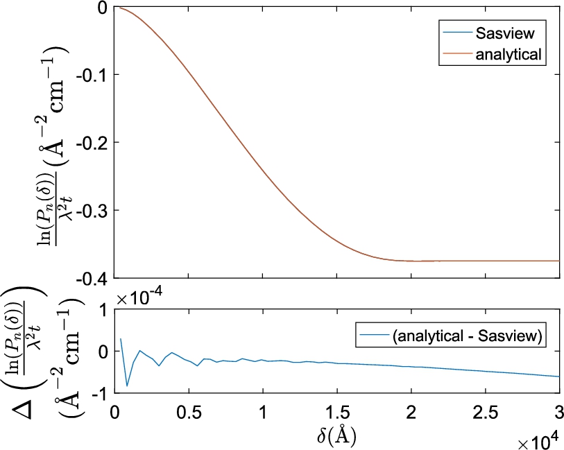
Plot of the numerically Hankel transformed SAS model of a sphere in SasView and the analytical projected correlation function of a sphere. Identical parameters were used for both functions (R=10,000 Å, φ=0.01, Δρ=5×10−6 Å−2). The top figure shows the 2 curves superimposing almost exactly; the difference is invisible at this scale, and therefore not significant when comparing to experiments. The bottom figure shows the difference between the 2 curves with a 104 magnification of the “absolute SESANS correlation function” axis scale.

The difference between the analytical equation and SasView’s numerical Hankel transform in Fig. 2 is a factor 1000 smaller than the magnitude of the absolute correlation values of the models themselves and a factor 100 smaller than typical experimental errors (see Figs 3 and 5 for examples). The oscillations in Fig. 2 at small δ are caused by too small Qmax and the deviation at large δ are caused by too high Qmin. This was tested only for the sphere model by varying the values for Qmin and Qmax. It is worth noting that Eq. (6) is more realistic than Eq. (25), since SESANS detectors have a finite size and thus detect a finite Q-range. Although the Qmax parameter in this paper does not currently represent this finite size, it could be made to do so in future versions of SasView, making data analysis using the numerical method presented here more realistic than data analysis using analytical functions.

3.2.Examples of fitting a numerical model to a data-set

In the following we validate our approach on experimental data, which have been acquired at the SESANS instrument in Delft [23]. These measurements used neutrons of λ=2.11 Å with a measurable δ-range of 10 nm to 20 μm. Fits were performed on several sets of experimental data. The solid sphere model (Eq. (24)) was applied to SESANS data of R=1 μm polystyrene spheres (NIST traceable standard) dissolved in 59% H₂O and 41% D₂O (sample provided by M. Strobl [29]) (Fig. 3). The fit correctly assigns a value of approximately R=1 μm (=10,000 Å) to the spheres. The sphere model, in combination with a log-normal distribution (Eq. (26)) for R, was applied to SESANS data of a dispersion of NILAC fat-free milk powder in D₂O (powder sample provided by NIZO Research, Netherlands) (Fig. 4). The powder consists of highly polydisperse casein micelles [31,33].

(26)PDF(x)=12πxΔxe(−ln(x/x0))22(Δx)2

with x the polydisperse quantity, Δx its standard deviation and x0 its mean value. Since log-normal distributions have long tails, the fitted value for R (431 Å) is much lower than the one obtained when fitting without any size distribution (1200 Å, not shown).

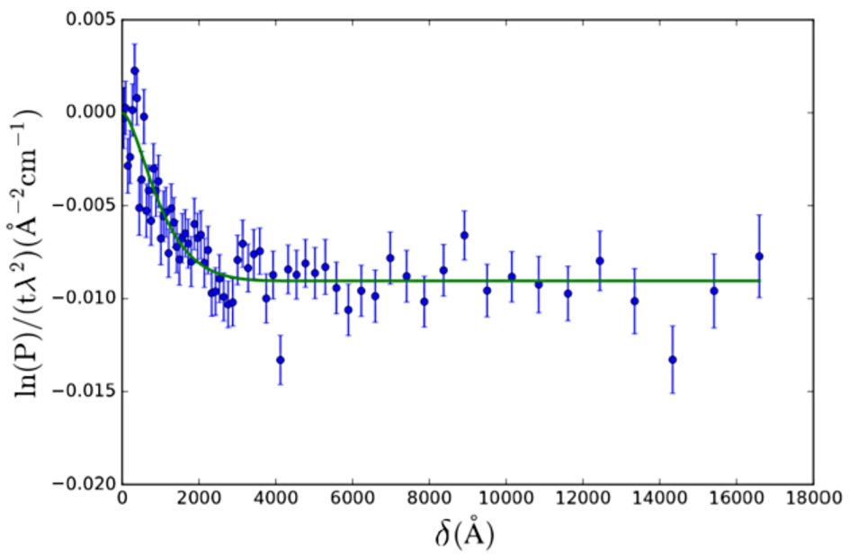
Fig. 3.

SESANS data of R=1 μm spherical poly-styrene colloids in D₂O. The SAS model used is the solid sphere (Eq. (24)). Fitted values are: R=(1040±10) Å and φ=(3.30±0.03)×10−2. Δρ was fixed at 2×10−6 Å−2. Data from M. Strobl et al. [29].

SESANS data of R=1 μm spherical poly-styrene colloids in D2O. The SAS model used is the solid sphere (Eq. (24)). Fitted values are: R=(1040±10) Å and φ=(3.30±0.03)×10−2. Δρ was fixed at 2×10−6 Å−2. Data from M. Strobl et al. [29].

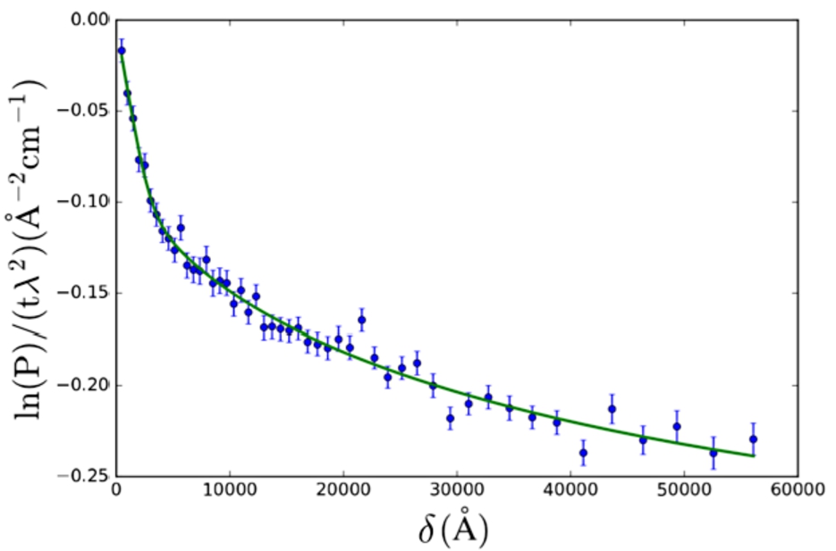
Fig. 4.

SESANS data of Nilac fat-free milk powder in D₂O. The SAS model used is the solid sphere (Eq. (24)) with lognormal polydispersity (Eq. (26)) of the radius. Fitted values are: R=(470±30) Å, Δρ=(0.76±0.02)×10−6 Å−2. PDI was fixed at 0.50 (σ/μ) (estimate by NIZO) and φ was fixed at 0.1 (estimate from Nilac bulk density and mass percentage in sample). Data from J.H. Bakker.

SESANS data of Nilac fat-free milk powder in D2O. The SAS model used is the solid sphere (Eq. (24)) with lognormal polydispersity (Eq. (26)) of the radius. Fitted values are: R=(470±30) Å, Δρ=(0.76±0.02)×10−6 Å−2. PDI was fixed at 0.50 (σ/μ) (estimate by NIZO) and φ was fixed at 0.1 (estimate from Nilac bulk density and mass percentage in sample). Data from J.H. Bakker.

The polymeric gel model (Eq. (27), from [28]) was applied to SESANS data of a gel (yogurt) of NILAC fat-free milk powder in D₂O (powder sample provided by NIZO Research, Netherlands) (Fig. 5). This sample is a dispersion of casein micelles in D₂O treated with glucono δ-lactone (GDL) to create a yogurt-like substance. The resulting structure has been previously described as a self-affine random medium [2,14,15]. Here we selected a SAS model which approximates the expected structure of the sample (casein micelles connected by a network of gel fibres).

(27)I(Q)=IL(0)(1+D+13ξ2Q2)D/2+IG(0)e−(RG2Q23)

where IL(0) and IG(0) are the absolute scattered intensities at Q=0 for the Lorentzian (gel) and Gaussian (polymer) contributions, respectively. D is the mass fractal dimension of the gel, ξ is its persistence length, and RG is the average radius of gyration of polymer clusters. The fit shows that most of the scattering is accounted for by the Lorentzian term (IL, the gel structure). This, in conjunction with the comparatively small contribution of the Gaussian term (IG, the casein micelles), indicates a high degree of gelation on the microscopic scale. The RG of the yogurt (≈ 2000 Å) is greater than the monodisperse R of the milk (≈ 1200 Å), most likely due to aggregation of the casein micelles before becoming “frozen in” in the gel structure [3,8,9].

Fig. 5.

SESANS data of Nilac fat-free milk powder in D₂O, treated to become yogurt. The SAS model used is the polymeric gel model (Eq. (27)). Fitted values are: IL=(4.3±2.0)×105 Å−1, IG=85±22 Å−1, D=2.38±0.06, RG=(2.0±0.2)×103 Å, ξ=(7.8±1.9)×104 Å. Data from J.H. Bakker.

SESANS data of Nilac fat-free milk powder in D2O, treated to become yogurt. The SAS model used is the polymeric gel model (Eq. (27)). Fitted values are: IL=(4.3±2.0)×105 Å−1, IG=85±22 Å−1, D=2.38±0.06, RG=(2.0±0.2)×103 Å, ξ=(7.8±1.9)×104 Å. Data from J.H. Bakker.

3.3.Example of fitting multiple models to a data-set

Two models were fitted to SESANS data of 70 nm radius spherical core-shell colloids with poly-styrene (PS) core and poly-ethylene oxide (PEO) corona in D₂O (data from K. v. Gruijthuijsen et al. [32]).The form factors used were those of solid spheres (Eq. (24)) and core-shell spheres (Eq. (28)),

(28)F(Q,Rs,Rc)2=3φ4πRs3(4πRc3(Δρ)scj1(QRc)QRc+4πRs3(Δρ)smj1(QRs)QRs)2,

where Δρsc=ρs−ρc and Δρsm=ρs−ρm. ρc, ρs and ρm are the scattering length densities of the core, shell and medium (solvent), respectively. Rc and Rs are the radii of the core and shell, respectively. In order to take the inter-particle correlations due to the high volume fraction into account, both form factors were multiplied by the hard-sphere structure factor (Eq. (29))

(29)S(Q)=11+24φX(Q)Rs

with Rs the “hard sphere radius”, and

(30)X(Q)=αK0(A)+βK1(A)+φα2·K3(A),(31)K0(A)=j1(A),K1(A)=2Asin(A)+(2−A2)cos(A)−2A3,(32)K3(A)=−A4cos(A)+4·[(3A2−6)cos(A)+(A3−6A)sin(A)+6]A5,(33)A=2QRHS,α=(1+2φ)2(1−φ)4,β=−6φ(1+φ/2)2(1−φ)4.

The fit to the data is shown in Fig. 6 and the resulting model parameters are given in Table 1. The colloids were designed to become positively charged on their exterior surface when dispersed in water. In the sample used for this example, the colloids’ charges were assumed to be fully screened, resulting in hard-sphere interactions only. The fits clearly show that simplifying the form factor for the colloids to solid spheres does not give a good fit; when using a core-shell form factor instead, the fit to the model describes the data well.

Fig. 6.

SESANS data of core-shell colloids with a poly-styrene (PS) core and poly-ethylene oxide (PEO) shell in D₂O. The data is fitted with the solid sphere (Eq. (24), red) and the core-shell sphere (Eq. (28), green) form factor. Both SAS models were multiplied by the hard sphere structure factor (Eq. (29)). Model fit parameter values are given in Table 1. Data from K. v. Gruijthuijsen et al. [32].

SESANS data of core-shell colloids with a poly-styrene (PS) core and poly-ethylene oxide (PEO) shell in D2O. The data is fitted with the solid sphere (Eq. (24), red) and the core-shell sphere (Eq. (28), green) form factor. Both SAS models were multiplied by the hard sphere structure factor (Eq. (29)). Model fit parameter values are given in Table 1. Data from K. v. Gruijthuijsen et al. [32].

Table 1

Fit parameter values for the multi-model fit (Fig. 6). ρsolvent was kept fixed

Fit model	Sphere	Core-shell
Rcore (Å)	703 ± 6	508 ± 24
Rshell (Å)		748 ± 35
ρcore (10−6 Å−2)	2.46 ± 0.01	0.28 ± 0.38
ρshell (10−6 Å−2)		5.61 ± 0.22
ρsolvent (10−6 Å−2)	6.4
ϕ	0.377 ± 0.008	0.338 ± 0.007

Fig. 7.

SANS (top) and SESANS (bottom) data of casein micelles in D₂O using the double power law scattering function (Eq. (34)). For this fit, all parameter values of the model, except for the SANS background, were linked between data-sets. The model fit parameter values are given in Table 2. Data from B. Tian [30].

SANS (top) and SESANS (bottom) data of casein micelles in D2O using the double power law scattering function (Eq. (34)). For this fit, all parameter values of the model, except for the SANS background, were linked between data-sets. The model fit parameter values are given in Table 2. Data from B. Tian [30].

3.4.Examples of simultaneous constrained fitting of SANS and SESANS data

A simultaneous constrained fit was performed on SANS and SESANS data of spray-dried calcium caseinate micelles in D₂O (data from B. Tian, [30]). The data-sets were fitted with a double power law scattering function (Fig. 7).

(34)I(Q)=AQ−m1if Q⩽Qc,CQ−m2if Q>Qc,

where C=AQcm2−m1. A and C are the scale factors for the power laws, m1 and m2 the two exponents at different length scales, and Qc the critical Q value separating the two power laws. The fit parameters are listed in Table 2. The fit indicates a cross-over between characteristic length scales at Q=9×10−4 Å−1. The value of m1 (1.37) indicates that the larger structures in the sample are either cylinders or strands, or very open networks. The value of m2 (2.95) suggests that the structures at shorter length scales are extremely rough or consist of collapsed polymer globules. The difference between the SANS and SESANS fit is only in the value of A, which corresponds to the I0 value for the low-Q power law. These samples are known to aggregate over time, and since SANS was performed after SESANS (on the same sample) the higher value of A could be due to aggregation of small particles into larger clusters.

USANS and SESANS data of poly-styrene spheres in D₂O (data from C. Rehm et al. [21]) were also analyzed using simultaneous/constrained fitting. The data-sets were fitted with a solid sphere form factor (Fig. 8) and the fit parameters are listed in Table 3. It should be noted that the USANS and SESANS measurements were not done on the same sample: 2 samples (1 for USANS, 1 for SESANS) were prepared using the same recipe, but were not taken from the same batch. Also, the SESANS sample was synthesized much longer in advance of the experiment than the USANS one. Due to the size of the particles, this led to significant sedimentation of the SESANS sample. For SESANS, multiple scattering correction is included in the data analysis [2,24]. This is not the case for USANS [25] and SasView does not take multiple scattering into account for SANS. These three factors (different samples, sedimentation, and multiple scattering correction) may explain the factor of 5 difference in φ. The fitted value for R (≈ 21300 Å) agrees well with the published data.

Table 2

Fit parameter values for the simultaneous fit of SANS and SESANS of casein micelles in D₂O (Fig. 7), using the double power law scattering function (Eq. (34)). Among the parameters, only Qc, m1 and m2 were constrained to be the same for both, SANS and SESANS, data sets. A and C were fitted without linking. Background (bkg) is a fit parameter only for SANS and was set to 0 for SESANS. SasView was unable to generate error estimates for this fit

Fit model	SANS	SESANS
A	23.0	18.6
C	0.0009	0.0007
Qc (Å−1)	9 × 10 -4
m1	1.19
m2	2.95
bkg (Å−1)	0.05	0

Fig. 8.

USANS (top) and SESANS (bottom) data of polystyrene micro-spheres in D₂O using the solid sphere form factor (Eq. (24)). For this fit, only R is constrained to be the same for both data sets, background (bkg) is only a fit parameter for USANS, Δρ was fixed and φ was fitted freely. For the USANS fit, a “slit smearing” resolution function with Γ1/2=2×10−5 was used. The derived parameter values are given in Table 3. Data from C. Rehm et al. [21].

USANS (top) and SESANS (bottom) data of polystyrene micro-spheres in D2O using the solid sphere form factor (Eq. (24)). For this fit, only R is constrained to be the same for both data sets, background (bkg) is only a fit parameter for USANS, Δρ was fixed and φ was fitted freely. For the USANS fit, a “slit smearing” resolution function with Γ1/2=2×10−5 was used. The derived parameter values are given in Table 3. Data from C. Rehm et al. [21].

Table 3

Fit parameter values for the simultaneous fit of USANS and SESANS of poly-styrene spheres in D₂O using the solid sphere form factor (Eq. (24)) (Fig. 8). R is linked. Δρ is fixed. φ is fitted without linking. Background (bkg) is only a fit parameter for SANS and was set to 0 for SESANS

Fit parameter	USANS	SESANS
R (Å)	21295 ± 22
Δρ (10−6 Å−2)	1.3
φ	0.293a	(6.30±0.03)×10−2
bkg	500a	0

^aSasView was unable to determine errors for these fit parameter values.

4.Conclusion

The validation of the numerical Hankel transform of a solid sphere against its projected correlation function showed excellent agreement and demonstrates that the numerical Hankel transform is, by extension, reliable for other SAS models. Fitting using single and multiple data-sets, in batch mode or with constrained fitting parameters has been proven to work without errors and examples of data analyses have been provided. SasView can now be used to analyze SESANS experimental data.

Acknowledgements

The authors would like to thank the SasView development team for their support in enabling user-friendly SESANS data analysis. Of the members of the SasView team, special thanks go to dr. J.R. (Jeffery) Krzywon for help with understanding the SasView code structure in the early stages of the project, dr. A.J. (Andrew) Jackson for keeping a broad perspective and the brief, yet extremely fruitful discussion leading to the understanding that resolution functions are coordinate transforms, dr. P.A. (Paul) Kienzle for extensive discussions and assistance integrating the SESANS routine into the SasView code-base, and P. Rozyczko and W. Potrzebowski for help with GUI integration and ensuring code stability. This work benefited from the use of the SasView application, originally developed under NSF award DMR-0520547. The USANS data presented in this paper was measured on the BT-5 instrument at NCNR (NIST) and the SANS data was measured on the Larmor instrument at ISIS (RAL).

SasView contains code developed with funding from the European Union’s Horizon 2020 research and innovation programme under the SINE2020 project, grant agreement No 654000. The authors acknowledge Nederlandse Organisatie voor Wetenschappelijk Onderzoek Groot grant no. LARMOR 721.012.102.

References

[1]	R. Andersson, W.G. Bouwman, S. Luding and I.M. De Schepper, Stress, strain, and bulk microstructure in a cohesive powder, Physical Review E – Statistical, Nonlinear, and Soft Matter Physics 77: (5) ((2008) ), 051303. doi:10.1103/PhysRevE.77.051303.
[2]	R. Andersson, L.F. van Heijkamp, I.M. de Schepper and W.G. Bouwman, Analysis of spin-echo small-angle neutron scattering measurements, Journal of Applied Crystallography 41: (5) ((2008) ), 868–885. doi:10.1107/S0021889808026770.
[3]	G.V. Bhaskar, O.H. Campanella and P.A. Munro, Effect of agitation on the coagulation time of mineral acid casein curd: Application of Smoluchowski’s orthokinetic aggregation theory, Chemical Engineering Science 48: (24) ((1993) ), 4075–4080. doi:10.1016/0009-2509(93)80252-L.
[4]	W.G. Bouwman, J. Plomp, V.O. de Haan, W.H. Kraan, A.A. van Well, K. Habicht, T. Keller and M. Theo Rekveldt, Real-space neutron scattering methods, Nuclear Instruments and Methods in Physics Research, Section A: Accelerators, Spectrometers, Detectors and Associated Equipment 586: (1) ((2008) ), 9–14. doi:10.1016/j.nima.2007.11.045.
[5]	W.G. Bouwman, R. Pynn and M.T. Rekveldt, Comparison of the performance of SANS and SESANS, Physica B: Condensed Matter 350: (1) ((2004) ), E787–E790. doi:10.1016/j.physb.2004.03.205.
[6]	W.G. Bouwman, O. Uca, S.V. Grigoriev, W.H. Kraan, J. Plomp and M.T. Rekveldt, First quantitative test of spin-echo small-angle neutron scattering, Applied Physics A: Materials Science and Processing 74: (Suppl. I) ((2002) ), s115–s117. doi:10.1007/s003390101081.
[7]	R.M. Dalgliesh, S. Langridge, J. Plomp, V.O. De Haan and A.A. Van Well, Offspec, the ISIS spin-echo reflectometer, Physica B: Condensed Matter, 406: ((2011) ), 2346–2349. doi:10.1016/j.physb.2010.11.031.
[8]	C.G. De Kruif, Casein micelle interactions, International Dairy Journal 9: (3–6) ((1999) ), 183–188. doi:10.1016/S0958-6946(99)00058-8.
[9]	C.G. de Kruif, Supra-aggregates of casein micelles as a prelude to coagulation, Journal of Dairy Science 81: (11) ((2010) ), 3019–3028. doi:10.3168/jds.s0022-0302(98)75866-7.
[10]	P. Debye, H.R. Anderson and H. Brumberger, Scattering by an inhomogeneous solid. II. The correlation function and its application, Journal of Applied Physics 28: (6) ((1957) ), 679–683. doi:10.1063/1.1722830.
[11]	P. Debye and A.M. Bueche, Scattering by an inhomogeneous solid, Journal of Applied Physics 20: (6) ((1949) ), 518–525. doi:10.1063/1.1698419.
[12]	R. Gähler, R. Golub, K. Habicht, T. Keller and J. Felber, Space-time description of neutron spin echo spectrometry, Physica B: Condensed Matter 229: (1) ((1996) ), 1–17. doi:10.1016/S0921-4526(96)00509-1.
[13]	T. Keller, R. Gähler, H. Kunze and R. Golub, Features and performance of an NRSE spectrometer at BENSC, Neutron News, 6: (3) ((1995) ), 16–17. doi:10.1080/10448639508217694.
[14]	L. Klimeš, Estimating the correlation function of a self-affine random medium, Pure and Applied Geophysics 159: (7–8) ((2002) ), 1833–1853. doi:10.1007/s00024-002-8711-1.
[15]	L. Klimeš, Correlation functions of random media, Pure and Applied Geophysics 159: (7–8) ((2002) ), 1811–1831. doi:10.1007/s00024-002-8710-2.
[16]	J. Kohlbrecher and A. Studer, Transformation cycle for spherical symmetric correlation functions, projected correlation function and small angle scatteringas implemented in SASfit, Journal of Applied Crystallography 50: ((2017) ), 1395–1403. doi:10.1107/S1600576717011979.
[17]	T. Krouglov, I.M. De Schepper, W.G. Bouwman and M.T. Rekveld, Real-space interpretation of spin-echo small-angle neutron scattering, Journal of Applied Crystallography 36: (1) ((2003) ), 117–124. doi:10.1107/S0021889802020368.
[18]	A. Kusmin, W.G. Bouwman, A.A. van Well and C. Pappas, Feasibility and applications of the spin-echo modulation option for a small angle neutron scattering instrument at the European Spallation Source, Nuclear Instruments and Methods in Physics Research Section A: Accelerators, Spectrometers, Detectors and Associated Equipment 856: ((2017) ), 119–132. doi:10.1016/j.nima.2016.12.013.
[19]	S.R. Parnell, A.L. Washington, K. Li, H. Yan, P. Stonaha, F. Li, T. Wang, A. Walsh, W.C. Chen, A.J. Parnell, J.P.A. Fairclough, D.V. Baxter, W.M. Snow and R. Pynn, Spin echo small angle neutron scattering using a continuously pumped 3He neutron polarisation analyser, Review of Scientific Instruments 86: (2) ((2015) ), 023902. doi:10.1063/1.4909544.
[20]	J. Plomp, V.O. de Haan, R.M. Dalgliesh, S. Langridge and A.A. van Well, Neutron spin-echo labelling at OffSpec, an ISIS second target station project, Thin Solid Films 515: (14 Spec. Iss.) ((2007) ), 5732–5735. doi:10.1016/j.tsf.2006.12.129.
[21]	C. Rehm, J. Barker, W.G. Bouwman and R. Pynn, DCD USANS and SESANS: A comparison of two neutron scattering techniques applicable for the study of large-scale structures, Journal of Applied Crystallography 46: (2) ((2013) ), 354–364. doi:10.1107/S0021889812050029.
[22]	M.T. Rekveldt, Novel SANS instrument using neutron spin echo, Nuclear Instruments and Methods in Physics Research Section B: Beam Interactions with Materials and Atoms 114: (3–4) ((1996) ), 366–370. doi:10.1016/0168-583X(96)00213-3.
[23]	M.T. Rekveldt, J. Plomp, W.G. Bouwman, W.H. Kraan, S. Grigoriev and M. Blaauw, Spin-echo small angle neutron scattering in Delft, Review of Scientific Instruments 76: (3) ((2005) ), 033901. doi:10.1063/1.1858579.
[24]	M.Th. Rekveldt, W.G. Bouwman, W.H. Kraan, O. Uca, S.V. Grigoriev, K. Habicht and T. Keller, Elastic neutron scattering measurements using Larmor precession of polarized neutrons, in: Neutron Spin Echo Spectroscopy Viscoelasticity Rheology, F. Mezei, C. Pappas and T. Gutberlet, eds, Lecture Notes in Physics, Vol. 601: , Springer, Berlin, (2007) , pp. 87–99. ISBN 978-3-540-44293-6. doi:10.1007/3-540-45823-9.
[25]	J. Schelten and W. Schmatz, Multiple-scattering treatment for small-angle scattering problems, Journal of Applied Crystallography 13: (4) ((1980) ), 385–390. doi:10.1107/s0021889880012356.
[26]	Science and Technology Facilities Council, ISIS Target Station 2 – Offspec, https://www.isis.stfc.ac.uk/Pages/Offspec.aspx, http://www.isis.stfc.ac.uk/instruments/Offspec/.
[27]	Science and Technology Facilities Council, ISIS Target Station 2 – Larmor, https://www.isis.stfc.ac.uk/Pages/Larmor.aspx.
[28]	M. Shibayama, T. Tanaka and C.C. Han, Small angle neutron scattering study on poly(N-isopropyl acrylamide) gels near their volume-phase transition temperature, Journal of Chemical Physics 97: (9) ((1992) ), 6829–6841. doi:10.1063/1.463636.
[29]	M. Strobl, B. Betz, R.P. Harti, A. Hilger, N. Kardjilov, I. Manke and C. Gruenzweig, Wavelength-dispersive dark-field contrast: Micrometre structure resolution in neutron imaging with gratings, Journal of Applied Crystallography 49: (2) ((2016) ), 569–573. doi:10.1107/S1600576716002922.
[30]	B. Tian, Structure and Dynamics of Fibrous Calcium Caseinate Gels Studied by Neutron Scattering, TU Delft University, Delft, (2020) . ISBN 9789402818857. doi:10.4233/uuid:90ed83af-4eca-45bc-af1a-816db85814d9.
[31]	R.H. Tromp and W.G. Bouwman, A novel application of neutron scattering on dairy products, Food Hydrocolloids 21: (2) ((2007) ), 154–158. doi:10.1016/j.foodhyd.2006.02.008.
[32]	K. van Gruijthuijsen, W.G. Bouwman, P. Schurtenberger and A. Stradner, Direct comparison of SESANS and SAXS to measure colloidal interactions, EPL (Europhysics Letters) 106: (2) ((2014) ), 28002. doi:10.1209/0295-5075/106/28002.
[33]	L.F. Van Heijkamp, I.M. De Schepper, M. Strobl, R. Hans Tromp, J.R. Heringa and W.G. Bouwman, Milk gelation studied with small angle neutron scattering techniques and Monte Carlo simulations, Journal of Physical Chemistry A 114: (7) ((2010) ), 2412–2426. doi:10.1021/jp9067735.
[34]	L.F. Van Heijkamp, A.M. Sevcenco, D. Abou, R. Van Luik, G.C. Krijger, P.L. Hagedoorn, I.M. De Schepper, B. Wolterbeek, G.A. Koning and W.G. Bouwman, Spin-echo small angle neutron scattering analysis of liposomes and bacteria, Journal of Physics: Conference Series, 247: ((2010) ), 012016. doi:10.1088/1742-6596/247/1/012016.
[35]	A.L. Washington, X. Li, A.B. Schofield, K. Hong, M.R. Fitzsimmons, R. Dalgliesh and R. Pynn, Inter-particle correlations in a hard-sphere colloidal suspension with polymer additives investigated by Spin Echo Small Angle Neutron Scattering (SESANS), Soft Matter 10: (17) ((2014) ), 3016–3026. doi:10.1039/c3sm53027b.