
McStas (i): Introduction, use, and basic principles for ray-tracing simulations
Abstract
We present an overview of, and an introduction to, the general-purpose neutron simulation package McStas. We present the basic principles behind Monte Carlo ray-tracing simulations of neutrons performed in the package and present a few simple examples. We present the implementation of McStas, the status of the package and its use in the neutron community. Finally, we briefly discuss the planned development of the package.
1.Introduction
Over the last decades, Monte Carlo ray-tracing simulation has become increasingly important for investigating the performance of neutron scattering instrumentation. Few neutron instruments are being built before undergoing a thorough investigation by simulation. In particular, the powerful spallation neutron sources in North America (SNS) [54] and Japan (J-PARC MLF) [49], the upgrade of the UK source (ISIS TS-2) [48], and the coming European Spallation Source (ESS) [47] have heavily utilized neutron simulation software, thereby also pushing the development of the simulation methods.
At the end of last century, neutron instrumentation ray-tracing simulations were performed using home-made monolithic codes. While fairly successful, this approach suffered from limited development ressources – with potential problems of quality assurance – while still creating a vast amount of duplicated effort between different projects and facilities. One exception from the monolithic approach was the general-purpose neutron simulation package NISP [7,52,57] released 1994/95, based on the earlier MCLIB subroutine library from 1978/1980 [17,18]. However, NISP never reached a critical mass of user community worldwide.
Almost simultanously, at the turn of the century, four general simulation packages were launched, following the NISP philosophy, but on more modern software platforms:
In the view of the authors of this paper, the state of the art of currently available neutron Monte Carlo ray-tracing packages are summarized in Table 1, including points of view on differences and main advantages and disadvantages.
Table 1
Overview of state of the art in Monte Carlo ray-tracing, with main advantages and disadvantages of the most widely used packages
| Package | Plusses | Minusses |
| VITESS | ∙ Easy for beginners – no code to write. ∙ Use of pipes gives automatically parallel execution. ∙ Is on track to become hosted at FZJ. | ∙ Modules historically written without common structure requirement/standard. ∙ Hard to modify at the physics/module level as a user. ∙ Open source, but without open software repository. ∙ Key staff has at periods had limited backing from hosting institution. |
| RESTRAX SIMRES | ∙ Has mode for “upstream” simulations from sample to source. Gives a clear speed boost for sparse phase-space simulations. ∙ Historically specialized for TAS. | ∙ Historically specialized for TAS. ∙ Open source, but without open software repository. ∙ Only few developers |
| NISP | ∙ No assumption that instruments should be linear. Any volume can scatter to any volume. ∙ Monte Carlo engine derived from early MCNP. | ∙ No assumption that instruments should be linear. (Intrinsically demanding/slow.) ∙ Monte Carlo engine derived from early MCNP. ∙ Legacy Fortran program with unspecified license terms. ∙ Only few developers |
| McVine | ∙ Automatically enherits much functionality from McStas. ∙ Instrument description written in pure Python. (Industry standard.) ∙ Interfaces with physics models written in Python/c++ ∙ Object-oriented with separated physics/geometry ∙ Open source (BSD) with open repository. | ∙ Instrument description written in pure Python. (Not a dedicated solution for neutron scatterers.) ∙ Interfaces with physics models written in Python/c++ ∙ Due to object-oriented nature, components only interact via the neutron ∙ Not widely used outside US neutron scattering. ∙ Only few developers. |
| RAMP | ∙ New kid on the block. ∙ Intrinsically GPU-capable. ∙ Written in pure Python. ∙ Open Source with open repository. | ∙ New kid on the block, i.e. short history so far. ∙ Functionality so far limited. ∙ Order of magnitude GPU speedup is not yet achieved. |
| McStas | ∙ Flexible, users can interact at instrument, component and c-code level. ∙ True Open Source from the beginning, has open repository, many user contributions. ∙ New functionality can be added through short, modular c-code. ∙ Several developers working in parallel for almost full duration of project history. ∙ Parallelised using industry-standard MPI solution. (GPU developments are under way.) ∙ Interfaces with many other codes e.g. MCNP, Mantid, iFit. | ∙ Extremely flexible, users can interact at instrument, component and c-code level. (Which may be error prone if many advanced features are combined.) ∙ True Open Source from the beginning, many user contributions. (There are however requirements for code inclusion.) |
Based on the need for instrument developments, the early use of the software packages concentrated on simulating neutron optics, especially guide systems, and concepts for full instruments, including instrument resolutions.
A huge effort was performed in the beginning of this century with systematic comparison between simulation results of guides and optics in different packages and to some extent with actual measured data [58,69]. This work served strongly to track down tricky numerical errors, to increase confidence in the packages themselves, and to establish the ray-tracing technique as such.
With the aim of being able to simulate complete virtual experiments, the last decade has seen a growing demand for – and development of – a suite of scattering sample components.
This is the first article in a series of short reviews of the McStas package – with the planned future articles described in Section 6. For this reason, we will here review the general expressions used for Monte Carlo ray-tracing simulations of neutron scattering, In addition, we will discuss the implementation of the McStas system, its utilization and user community, and the planned future development of the package.
We have aimed this article for neutron scatterers and software developers alike, and we thus begin with a few introductory paragraphs on the nature of neutrons and on the ray-tracing technique. Most material presented here, and other related information, can be found also in the user and component manual for McStas [51].
2.The mathematics of Monte Carlo ray-tracing simulations for slow neutrons
Monte Carlo simulations are in general a way to perform approximate solutions to complex problems by use of random sampling, thereby performing numerical experiments. The first known example of such a method is that of the Buffon needle problem [46] first posed in the 18th century by Georges-Louis Leclerc, Comte de Buffon:
“Suppose we have a floor made of parallel strips of wood, each the same width, and we drop a needle onto the floor. What is the probability that the needle will lie across a line between two strips?”
As explained in a wikipedia article [56], the thinking behind that numerical experiment can in fact be used to construct a Monte Carlo algorithm for the estimation of π. In terms of an actual mathematical algorithm, and later code for computers, the first formulation was in fact to facilitate calculations of neutron physics for the Manhattan project [29].
As with all stochastic methods, Monte Carlo methods are prone to statistical variances. To reduce the statistical errors, a number of variance reduction methods have been designed, of which we here mention two. In Stratified sampling, one divides the parameter space up into mutually exclusive strata, and sample a given amount of each stratum. In Importance sampling, one will choose to sample more often in regions more important for the final result. As an analogy, to calculate the average height over sea level of a landscape, one would map the ragged mountain slopes more carefully than the still water in the mountain lake.
The method relevant for neutron simulations is known as Monte Carlo ray-tracing. This is used to study objects which travel along a path (a ray), and can be (partially) absorbed or scattered into another direction, but not converted into other types of radiation. The most known example of this is visible light, and this type of ray-tracing is frequently used to generate realistic illumination in 3D computer graphics, see e.g. Pov-Ray [33].
2.1.The semiclassical representation of neutron coordinates
In neutron ray-tracing simulations a neutron is represented semiclassically by simultaneously well-defined position, r, velocity, v, time, t, and all three components of the neutron spin vector, s.
Formally, this approach violates the laws of quantum mechanics, in particular the Heisenberg uncertainty relations [28], given for pairs of conjugate position/momentum variables by
The validity of the semiclassical approach for neutron scattering is also discussed in detail in Ref. [30]. The similar issues with the semiclassical approximation of the neutron spin will be discussed in the future review on polarized scattering.
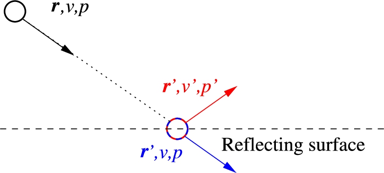
Fig. 1.
Neutron ray interacting with a reflecting surface: 1. The neutron begins with parameters
2.2.The weight factor
The physical unit of a neutron ray is neutron rate, or neutron intensity (s−1). On a typical neutron source, the emission rate can amount to 1015/s; an order of magnitude larger than the number of rays that can typically be simulated on a laptop in one year. For this reason, to simulate realistic values for neutron count numbers, a neutron ray in general represents more than a single physical neutron (per second). To accommodate this, each ray contains an additional parameter, the weight factor, p, with a unit of neutrons per second. When the ray begins at the source, p is typically 103/s to 109/s. The intensity of the given neutron ray is updated on interaction with components of the neutron instrument, see Fig. 1 for an illustration.
As one example of importance sampling, the weight factor is manipulated through the simulation. For example, when some physical neutrons are “lost” due to e.g. finite reflectivity or absorption, the simulated ray will in general continue in the simulations, while p is adjusted to reflect the correct average physical behaviour. When (if) the neutron ray reaches the detector, p may in practice be less than 1/s. Turning again to Fig. 1, using importance sampling by describing the reflected beam only will not neglect the physical influence of absorption, since we ensure conservation of intensity, i.e.
We proceed along this line of reasoning to calculate the neutron intensity in a beam. Consider a neutron component at a surface perpendicular to the beam. The neutron intensity is given by the sum of all simulated rays reaching this surface:
Often, there is only one non-trivial event to consider. This may, e.g., be the case for a neutron beam being attenuated by absorption. Here, each neutron ray either survives or is lost. Absorbed neutrons are typically not simulated (
When a Monte Carlo branch point is reached (selection between several events), we have
2.3.Neutron moderators and focusing
Consider a component that may send neutrons out in all directions, e.g. the moderator or the sample. Often in McStas, we choose uniform sampling when simulating all neutron directions. The sampling probability per solid angle is then:
Imagine a McStas moderator component, simulating a moderator that emits R neutrons per second, divided into N rays. The total intensity in the simulation is found from
2.4.Estimates of simulation uncertainty
In a simulation, like for real experiments, it is important to be able to estimate the statistical uncertainty. We here present a simple derivation of the uncertainty in simulations with weight factors.
Imagine M rays, all with weight factor p. Each ray is imagined to have an overall probability,
We now allow the rays to have different, but discrete, weight factors,
Now, let the simulations occur with rays of arbitrary weight factors,
2.5.Scaling to real-world statistics
In order to compare with real experiments, in particular when using simulated data as input to data analysis programs, simulated intensities must be converted to average integer counts using an imagined counting time, T. However, this time cannot be chosen to be arbitrarily high, since the data analysis program will assume
Let us now we quantify the effect of scaling with a counting time. The average count number is easily obtained by
If a series of simulated values need to be scaled by the same time, T, the maximum time is given by the smallest value of T that fulfills (22), or
In conclusion, the count-error-true simulation numbers are
This transformation to integer count numbers is not used in McStas, but must be applied as a post processing of the data after the simulations. Further work is, however, needed on the sampling strategies for future more efficient transformation of errorbars.
3.The concept and implementation of McStas
As also outlined in the introduction, the philosophy and mindset behind starting the McStas project, as laid out by K.N. Clausen, was to a large extent to minimize duplication of code and efforts by allowing code to be shared [26]. The main ideas that were implemented since the first version of McStas were:
Licensing should follow Open Source standards. Since version 1.8 McStas is released under the GNU General Public License v. 2.0. Earlier versions were licensed under a McStas- and RISØ specific license that was open, but did not allow redestribution.
The code should be modular to allowed sharing models of instrument parts between users. This evolved into the so-called components, explained below.
The syntax of the user-supplied instrument definition should be simple and powerful. For the development of the syntax details, K. Nielsen got input to the syntax, using pen and paper before writing any code, from the RISØ staff, in particular K. Lefmann and H.M. Rønnow wrote the first instrument and handful of components in this way.
The software concepts should first of all make sense to instrument scientists, allowing them to work in a way that felt almost like runnning an actual instrument
Documentation should as far as possible be embedded within the code
Simplicity and readability of the code should be preferred over performance.
McStas is implemented in a three-layered structure. The core system and run-time libraries take care of the compiling and execution of the program, user interface, and visualization of the results. The core and run-time c-code libraries typically come in a set of header and c-code files, such as
mccode-r.h and mccode-r.c, common to both McStas and McXtrace and containing functions for generating random numbers, routines for intersecting particle ray and geometrical objects etc.
mcstas-r.h and mcstas-r.c, containing physical constants for neutron physics, propagation routines with/without gravitation etc. (McXtrace has a similar set of files implementing X-ray physics)
interoff-lib.h and interoff-lib.c for handling of surface-polygon based geometries in GeomView OFF file format [41]
interpolation-lib.h and interpolation-lib.c, routines for interpolating in gridded and sparse datasets
ref-lib.h and ref-lib.c, routines for describing the physics of reflective super-mirror surfaces
read_table-lib.h and read_table-lib.c, routines for reading tabulated data from files
pol-lib.h and pol-lib.c, routines for handling polarized neutron transport
adapt_tree-lib.h and adapt_tree-lib.c, routines to define adaptive importance sampling schemes
These levels of code are only modified by a handful of system specialists. The core system also manages the main Monte-Carlo loop that in turn produces a specified number of neutron rays for the simulation.
Supplementing the core system run-time codes, a number of c-files are present to support individual McStas components, such as
monitor_nd-lib.h and monitor_nd-lib.c, supporting the very general Monitor_nD monitor component from Emmanuel Farhi, ILL
ESS_butterfly-lib.h, ESS_butterfly-geometry.c and ESS_butterfly-lib.c, supporting the ESS_butterfly source component
Geometry_functions.c, Union_functions.c and Union_initialization.c, supporting the Union component set by Mads Bertelsen, ESS DMSC
nxs.h and sginfo.h, supporting the Sample_nxs component from Mirko Boin, HZB
ess_source-lib.h and ess_source-lib.c, supporting the legacy ESS_moderator source component
chopper_fermi.h, chopper_fermi.c, general.h, general.c, intersection.h, intersection.c, vitess-lib.h and vitess-lib.h, supporting the Vitess_Chopperfermi component, ported from VitESS
The components are modular pieces of code. The McStas components are written in a unique domain-specific language, which is augmented using ANSI-C. A McStas component will typically be equivalent to a beam-optical component, such as a chopper, a collimator, a particular sample, or a detector (often called “monitor” in McStas). Sources and moderator are in McStas implemented as one combined component. Components are typically parametrised, e.g. with respect to size, in order to be of general use. The components will use the matematical tools for e.g. weight transformation and focusing, presented in Section 2.
The instrument is a description of a particular neutron scattering set-up. McStas operates at one instrument at a time. The instrument file contains a selection of components and their spatial position and orientation. The instrument is written fully in the McStas domain specific language, although ANSI-C may be used to augment the functionality. Also the instruments can be parametrised, for example to allow the scanning of a triple-axis instrument by changing a number of angles. Figure 2 illustrates the roles of system, components, and instrument file for a very simple time-of-flight instrument, consisting of a pulsed source, a guide, a chopper, and a time-of-flight detector.
Fig. 2.
The figure illustrates how the McStas (and McXtrace) codes are layered, including how user, developers and code generation mechanism interact with the various layers of code. The geometrical lay-out of the instrument to simulate is shown at the top panel, while the bottom panes represent the different interacting layers of McStas. The instrument file is shown fully in the large panel to the left; the figure is not to scale. Reproduced from [65].
![The figure illustrates how the McStas (and McXtrace) codes are layered, including how user, developers and code generation mechanism interact with the various layers of code. The geometrical lay-out of the instrument to simulate is shown at the top panel, while the bottom panes represent the different interacting layers of McStas. The instrument file is shown fully in the large panel to the left; the figure is not to scale. Reproduced from [65].](https://content.iospress.com:443/media/jnr/2020/22-1/jnr-22-1-jnr190108/jnr-22-jnr190108-g002.jpg)
When McStas is executed on an instrument file, the system compiles the information from the instrument file and the component library and produces an ANSI-C file. This is in turn compiled by a standard C-compiler to an executable code, which is called by the system. After the process has terminated, McStas collects the resulting data files, stores them in specified directories, and visualises the data upon request. Everything can be controlled from a user-friendly GUI interface, or by a scripting language.
McStas has a users manual and a component manual [51], both of which are very comprehensive documents. A more readily accessible documentation may be found in the project home page. Documentation of component functionality is furthermore embedded in the header of the component code. This documentation is e.g. used for the generation of online component help at the McStas home page [50].
4.Use and users of McStas
In its first two decades, McStas has seen a steady increase of users. We have chosen to illustrate this with a literature search. We have analyzed the 350 articles citing one (or more) of the basic McStas release articles, and by far most of these articles in fact represent simulation work done by the use of McStas.
In Fig. 3, we show the number of McStas-using articles as a function of publication year. We see that after a slow start (except for a spike in 2002), the publication rate reached 10/y in 2006 and 20/y in 2011. Since 2014, the number has been approx. 30/y, which is partly based on the large instrumentation work related to ESS.
Fig. 3.
The annual number of articles citing McStas shown as a function of publication year.
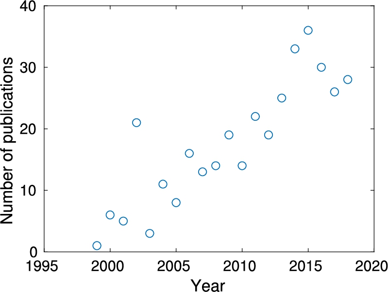
Fig. 4.
The number of articles citing McStas, divided into use categories, shown as a function of 5-year intervals.
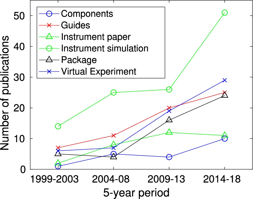
It is highly interesting to study what McStas has been used for, judging from this literature base. Figure 4 shows the six main use categories of the packages, distributed on 5-year periods. Although the overall use of McStas has increased by a factor 4 over the years, the distribution between the categories has remained remarkably constant. Let us present the themes one by one (all will be described in much more detail in later issues of this article series):
Components. These papers describe the simulations of individual beam-optical components, such as choppers, monochromators [36], lenses [14], or mirrors [59]. Around 5% of the articles fall in this category.
Guides. A particular application of McStas has been to study different guide systems, both generic guide geometries [20,40], and guide constructions for actual instruments [15,22]. Recently, tools have become available for semi-automatic optimization of guide geometries [4] and guide coatings [32], strongly enhancing the capabilities and speed of simulation-guided optimizations for guide designs. Around 20% of the McStas articles are in this category.
Instrument papers. This denotes the important papers describing the performance of an actual instrument. Such papers will typically obtain many citations, as they will be the standard reference for users of the instrument. Often, the use of McStas in these papers is related to prediction of flux on sample, and the calculation of resolution functions, both to be compared to the actual measured values. Approx. 10% of the McStas papers are instrument papers and represent instruments at the major facilities around the world, for example:
Instrument simulations. These articles represent the design work behind instruments, some of which are not yet built, and a few of which may never be built at all. This is a main category for McStas work, containing 35% of all articles. The simulations cover all facilities listed above, as well as:
the Algier reactor
the Argentine reactor
CSNS
Dhruva
ESS
HANARO
Dubna
LLB
PIK
As a separate task, McStas has been used in two demanding studies of the complete instrument suite for ESS, first to optimize the pulse structure [25], then to optimize the moderator geometry [2].
Virtual experiments. These articles represent the most advanced use of simulations, namely the performance of a full virtual experiment on a simulated instrument [13,27]. This has been used for the determination of accurate resolution functions [9,63], tools for teaching practical neutron scattering without the investment of beam time [62], for correcting for multiple scattering events in samples [5,12,13], and even for analysis of complete data sets [6,16,61,66]. Around 15% of the articles fall in this category.
Packages. These articles describe simulation packages, typically McStas, but also VITESS and RESTRAX have cited McStas, partially for the reason that these three packages have inspired and cross-fertilized each other over the last two decades. In addition, McStas has spawned an X-ray cousin (McXtrace) [21] and a He-scattering cousin [10]. Around 15% of the articles are in this category.
In addition to this bibliometric study, we have performed a survey of the McStas user community during the autumn of 2018. Ten questions were posed via the SurveyMonkey platform [42] in the period from November 6th 2018 to December 3rd 2018. All questions were voluntary/optional and contained the possibility of free-form input via an ‘other’ text field. In total 52 responses were received, out of which 47 filled demographic data. The full McStas user base is estimated to be approximately 400, based on the current 252 members of the McStas user mailinglist and knowing from experience that not all users register.
The main findings of the survey are that:
1. The McStas users are to a high degree running the most recent version of McStas, at the time of survey v. 2.4.1.
2. Linux is the dominant operating system, followed by Windows 10 and macOS. Some users are now running the Linux binaries under Windows 10 via the Windows Subsystem for Linux [44].
3. McStas users are distributed over all of the continents that have access to neutron facilities.
4. McStas users are mostly based at neutron facilities, but the package also finds use at universities and in industry.
5. Most users are now routinely using our modernised Python based gui and command-line utitlites.
6. The vast majority of McStas users are very happy about the McStas installation process, daily use and the available user support.
5.The future of McStas
As our user survey demonstrates, McStas is as a project alive and healthy with a 20 year long history of development and a stable user community. What separates McStas from the alternative simulation packages is mainly the applied code-generation technique, the quality of documentation and the strongly collaborative nature of the package, allowing users to contribute. To stay alive and healthy however, a sustained effort is needed in terms of manpower, resources, support and development.
The main focal points for the development in the coming years are:
1. Lower the typical release cycle of 12–18 months to 3–6 months. Updating more often lowers ‘time to market’ for new ideas, solutions and bug-fixes. McStas 2.5 was released in December 2018 and 2.5.1 will be released in the spring of 2019.
2. Make our test/validation effort more stringent and use more of a ‘continuous integration’ approach to testing. All components should have output test data that we can monitor against on a continuous basis. Today only a scalar numerical output defines a ‘test’ – in the future we would like to compare at a more detailed level of data in individual bins of individual monitors.
3. Enrich the sample library even further. A natural layer of growth is the Union [5] concept by Mads Bertelsen which allows to separate geometry and physical processes by defining an inner Monte Carlo loop (e.g. for describing complicated arrangements of matter in/around the sample area). The Union components should become complete in terms of describing all possible geometries and all possible physics, which is today not fully the case.
4. A modernization of the code generation layer is under way, which will allow us to move to a C-function based grammar rather than today’s #define-based approach.11 This will break certain backward-compatibility and move us to McStas v. 3.0
5. The modernized code-generation will ease the process of targeting modern GPU-based architectures.
6.The McStas review series
This article should be seen as an introduction to a series of McStas review papers. Planned themes in this series cover the main uses of McStas described above:
Components
Guide systems
Instrument simulations and virtual experiments
Modeling of scattering from samples
Simulation of polarized neutrons, including spin precession
Notes
1 The classical McStas code uses c-preprocessor [45] define instructions to locally change the meaning of a variable or parameter name. This means that e.g. a geometrical parameter symbol xwidth can be used by multiple components within the same instrument, but with a local meaning and without inconsistency.
Acknowledgements
It is a pleasure to thank everyone involved in the McStas project over the decades. In chronological order: K.N. Clausen, K. Nielsen, H.M. Rønnow, E. Farhi, P.-O. Åstrand, K. Lieutenant, P. Christiansen, E.B. Knudsen, U. Filges, J. Garde, and M. Bertelsen.
References
[1] | D.L. Abernathy, M.B. Stone, M.J. Loguillo, M.S. Lucas, O. Delaire, X. Tang, J.Y.Y. Lin and B. Fultz, Rev. Sci. Instr. 83: ((2012) ), 015114. doi:10.1063/1.3680104. |
[2] | K.H. Andersen, M. Bertelsen, L. Zanini, E.B. Klinkby, T. Schönfeldt, P.M. Bentley and J. Saroun, Optimization of moderators and beam extraction at the ESS, J. Appl. Cryst. 51: ((2018) ), 264. doi:10.1107/S1600576718002406. |
[3] | R.J. Barlow, Statistics, Wiley, (1999) . |
[4] | M. Bertelsen, Guide-Bot, Nucl. Instr. Meth. A ((2017) ). |
[5] | M. Bertelsen, T. Guidi and K. Lefmann, Expanding the McStas sample simulation logic with McStas Union components, 2019, in preparation. |
[6] | M. Boin, R.C. Wimpory, A. Hilger, N. Kardjilov, S.Y. Zhang and M. Strobl, Monte Carlo simulations for the analysis of texture and strain measured with Bragg edge neutron transmission, Journal of Physics Conference Series 340: ((2012) ), 012022. doi:10.1088/1742-6596/340/1/012022. |
[7] | L.L. Daemen, P.A. Seeger, T.G. Thelliez and R.P. Hjelm, A Monte Carlo tool for simulations of neutron scattering instruments, AIP Conference Proceedings 479: ((1999) ), 41–46. doi:10.1063/1.59486. |
[8] | S.A. Danilkin, M. Yethiraj, T. Saerbeck, F. Klose, C. Ulrich, J. Fujioka, S. Miyasaka, Y. Tokura and B. Keimer, TAIPAN: First results from the thermal triple-axis spectrometer at OPAL research reactor, Journal of Physics Conference Series 340: ((2012) ), 012003. doi:10.1088/1742-6596/340/1/012003. |
[9] | G. Eckold and O. Sobolev, Analytical approach to the 4D-resolution function of three axes neutron spectrometers with focussing monochromators and analysers, Nucl. Instr. Meth. A 752: ((2014) ), 54. doi:10.1016/j.nima.2014.03.019. |
[10] | S.D. Eder, A.K. Ravn, B. Samelin, G. Bracco, A. Salvador Palau, T. Reisinger, E.B. Knudsen, K. Lefmann and B. Holst, Zero-order filter for diffractive focusing of de Broglie matter waves, Phys. Rev. A 95: ((2017) ), 023618. doi:10.1103/PhysRevA.95.023618. |
[11] | G. Ehlers, A.A. Podlesnyak, J.L. Niedziela, E.B. Iverson and P.E. Sokol, The new cold neutron chopper spectrometer at the Spallation Neutron Source: Design and performance, Rev. Sci. Instr. 82: ((2011) ), 085108. doi:10.1063/1.3626935. |
[12] | E. Farhi, V. Hugouvieux, M.R. Johnson and W. Kob, J. Comp. Phys. 228: ((2009) ), 5251. doi:10.1016/j.jcp.2009.04.006. |
[13] | E. Farhi, V. Hugouvieux, M.R. Johnson and W. Kob, Virtual experiments: Combining realistic neutron scattering instrument and sample simulations, J. Comp. Phys. 228: ((2009) ), 5251. doi:10.1016/j.jcp.2009.04.006. |
[14] | H. Frielinghaus, J. Appl. Cryst. 42: ((2009) ), 681. doi:10.1107/S0021889809017919. |
[15] | R.M. Ibberson, Nucl. Instr. Meth. A 600: ((2009) ), 47. doi:10.1016/j.nima.2008.11.066. |
[16] | H. Jacobsen, S.L. Holm, M.-E. Lacatusu, A.T. Rømer, M. Bertelsen, M. Boehm, R. Toft-Petersen, J.-C. Grivel, S.B. Emery, L. Udby, B.O. Wells and K. Lefmann, Distinct nature of static and dynamic magnetic stripes in cuprate superconductors, Phys. Rev. Lett 120: ((2018) ), 037003. doi:10.1103/PhysRevLett.120.037003. |
[17] | M.W. Johnson, MCGUIDE: A thermal neutron guide simulation program, Rutherford and Appleton Laboratories report RL-80-065, 1980. |
[18] | M.W. Johnson and C. Stephanou, MCLIB: A library of Monte Carlo subroutines for neutron scattering problems, Rutherford Laboratory report RL-78-090, 1978. |
[19] | R. Kajimoto, M. Nakamura, Y. Inamura, F. Mizuno, K. Nakajima, S. Ohira-Kawamura, T. Yokoo, T. Nakjatani, R. Maruyama, K. Soyama, K. Shibata, K. Suzuya, S. Sato, K. Aizawa, M. Arai, S. Wakimoto, M. Ishikado, S. Shamoto, M. Fujita, H. Hiraka, K. Ohoyama, K. Yamada and C.H. Lee, J. Phys. Soc. Jpn. 80: ((2011) ), SB025. doi:10.1143/JPSJS.80SB.SB025. |
[20] | K.H. Klenø, K. Lieutenant, K.H. Andersen and K. Lefmann, Systematic performance study of common guide geometries, Nucl. Instr. Meth. A 696: ((2012) ), 75. doi:10.1016/j.nima.2012.08.027. |
[21] | E.B. Knudsen, A. Prodi, J. Baltser, M. Thomsen, P.K. Willendrup, M. Sanchez del Rio, C. Ferrero, E. Farhi, K. Haldrup, A. Vickery, R. Feidenhans’l, K. Mortensen, M.M. Nielsen, H.F. Poulsen, S. Schmidt and K. Lefmann, McXtrace: A Monte Carlo software package for simulating X-ray optics, beamlines and experiments, J. Appl. Cryst. 46: ((2013) ), 679. doi:10.1107/S0021889813007991. |
[22] | M.D. Le, D. Quinteros-Castro, R. Toft-Petersen, F. Groitl, M. Skoulatos, K.C. Rule and K. Habicht, Gains from the upgrade of the cold neutron triple-axis spectrometer FLEXX at the BER-II reactor, Nucl. Instr. Meth. A 729: ((2013) ), 220. doi:10.1016/j.nima.2013.07.007. |
[23] | W.-T. Lee, X.-L. Wang, J.L. Robertson, F. Klose and C. Rehm, Appl. Phys. A 74: ((2002) ), S1502. doi:10.1007/s003390201723. |
[24] | K. Lefmann, Physica B 385: (86) ((2006) ), 1083. doi:10.1016/j.physb.2006.05.372. |
[25] | K. Lefmann, K.H. Klenø, J.O. Birk, B.R. Hansen, S.L. Holm, E. Knudsen, K. Lieutenant, L. von Moos, M. Sales, P.K. Willendrup and K.H. Andersen, Simulation of a suite of generic long-pulse neutron instruments to optimize the time structure of the European Spallation Source, Rev. Sci. Instr. 84: ((2013) ), 055106. doi:10.1063/1.4803167. |
[26] | K. Lefmann and K. Nielsen, Neutron News 10: (3) ((1999) ), 20. doi:10.1080/10448639908233684. |
[27] | K. Lefmann, P.K. Willendrup, L. Udby, B. Lebech, K. Mortensen, J.O. Birk, K. Klenø, E. Knudsen, P. Christiansen, J. Saroun, J. Kulda, U. Filges, M. Konnecke, P. Tregenna-Piggott, J. Peters, K. Lieutenant, G. Zsigmond, P. Bentley and E. Farhi, Virtual experiments: The ultimate aim of neutron ray-tracing simulations, J. Neutr. Res. 16: ((2008) ), 97. doi:10.1080/10238160902819684. |
[28] | E. Merzbacher, Quantum Mechanics, 3rd edn, Wiley and Sons, (1997) . |
[29] | N. Metropolis, http://library.lanl.gov/la-pubs/00326866.pdf. |
[30] | F. Mezei, in: The Basic Physics of Neutron Scattering Experiments, Lecture Notes of the Introductory Course to the ECNS99, Report KFKI-1999-04/E, (1999) , pp. 27–39. |
[31] | K. Nakajima, S. Ohira-Kawamura, T. Kikuchi, M. Nakamura, R. Kajimoto, Y. Inamura, N. Takahashi, K. Atzawa, K. Suzuya, K. Shibata, T. Nakatani, K. Soyama, R. Maruyama, H. Tanaka, W. Kambara, T. Iwahasmi, Y. Itoh, T. Osakabe, S. Wakimoto, K. Kakurai, F. Maekawa, M. Harada, K. Oikawa, R.E. Lechner, F. Mezei and M. Arai, AMATERAS: A cold-neutron disk chopper spectrometer, J. Phys. Soc. Japan 80: ((2011) ), SB028. doi:10.1143/JPSJS.80SB.SB028. |
[32] | M.A. Olsen, M. Bertelsen and K. Lefmann, Optimizing neutron guides: Coating writer, J. Neutr. Res. ((2019) ). |
[33] | Pov-Ray – Persistence of Vision Pty. Ltd. (2004) , http://www.povray.org/download/. |
[34] | A. Radulescu, V. Pipich, H. Freilinghaus and M.S. Appavou, J. Phys. Conf. Ser. 351: ((2012) ), 12026. doi:10.1088/1742-6596/351/1/012026. |
[35] | J.A. Rodriguez, D.M. Adler, P.C. Brand, C. Broholm, J.C. Cook, C. Brocker, R. Hammond, Z. Huang, P. Hundertmark, J.W. Lynn, N.C. Maliszewskyj, J. Moyer, J. Orndorff, D. Pierce, T.D. Pike, G. Scharfstein, S.A. Smee and R. Vilaseca, MACS – a new high intensity cold neutron spectrometer at NIST, Measurement Science and Technology 19: ((2008) ), 034023. doi:10.1088/0957-0233/19/3/034023. |
[36] | J.R. Santisteban, J. Appl. Cryst. 38: ((2005) ), 934. doi:10.1107/S0021889805028190. |
[37] | J.R. Santisteban, M.R. Daymond, J.A. James and L. Edwards, J. Appl. Cryst. 39: ((2006) ), 812. doi:10.1107/S0021889806042245. |
[38] | J. Saroun and J. Kulda, Physica B 234–236: ((1997) ), 1102. doi:10.1016/S0921-4526(97)00037-9. |
[39] | J. Saroun and J. Kulda, SPIE Proc. 5536: ((2004) ), 124. doi:10.1117/12.560925. |
[40] | C. Schanzer, P. Böni, U. Filges and T. Hils, Advanced geometries for ballistic neutron guides, Nucl. Instr. Meth. A 529: ((2004) ), 63. doi:10.1016/j.nima.2004.04.178. |
[41] | See http://www.geomview.org and http://www.geomview.org/docs/html/OFF.html. |
[42] | |
[43] | See http://survey2018.mcstas.org for a complete, summarized survey report. |
[44] | |
[45] | See https://en.wikipedia.org/wiki/C_preprocessor for an explanation. |
[46] | See de l’Acad. Roy. des. Sciences (1733), 43–45; naturelle, générale et particulière Supplément 4 (1777), p. 46. |
[47] | See the ESS home page http://europeanspallationsource.se. |
[48] | See the ISIS home page https://www.isis.stfc.ac.uk/. |
[49] | See the J-PARC MFL home page https://j-parc.jp/researcher/MatLife/en/. |
[50] | See the McStas home page at http://www.mcstas.org. |
[51] | See the McStas User Manual and the Component Manual at http://www.mcstas.org/documentation/manual/. |
[52] | See the NISP home page http://paseeger.com. |
[53] | See the RESTRAX/SIMRES home page at http://neutron.ujf.cas.cz/restrax/. |
[54] | See the SNS home page https://neutrons.ornl.gov/sns. |
[55] | See the VITESS home page at https://www.helmholtz-berlin.de/forschung/oe/em/transport-phenomena/neutronmethods/vitess/. |
[56] | See the wikipedia article at https://en.wikipedia.org/wiki/Buffon%27s_needle. |
[57] | P.A. Seeger and L.L. Daemen, The neutron instrument simulation package, NISP, Proceedings of SPIE 5536: ((2004) ), 109–123. doi:10.1117/12.559817. |
[58] | P.A. Seeger, L.L. Daemen, E. Farhi, E.-T. Lee, L. Wang, L. Passel, J. Saroun and G. Zsigmond, Monte Carlo code comparisons for a model instrument, Neutron News 13: ((2002) ), 24–29. doi:10.1080/10448630208218491. |
[59] | J. Stahn, U. Filges and T. Panzner, Focusing specular neutron reflectometry for small samples, Europ. Phys. J. – Appl. Phys. 58: ((2012) ), 11001. doi:10.1051/epjap/2012110295. |
[60] | J.R. Stewart, J. Appl. Cryst. 42: ((2009) ), 69. doi:10.1107/S0021889808039162. |
[61] | S. Taminato et al., Real-time observations of lithium battery reactions-operando neutron diffraction analysis during practical operation, Scientific Reports 6: ((2016) ), 28843. doi:10.1038/srep28843. |
[62] | L. Udby et al., 2019, in preparation. |
[63] | L. Udby, P.K. Willendrup, E. Knudsen, C. Niedermayer, U. Filges, N.B. Christensen, E. Farhi, B.O. Wells and K. Lefmann, Analysing neutron scattering data using McStas virtual experiments, Nucl. Instr. Meth. A 634: ((2011) ), S138. |
[64] | P.K. Willendrup, E. Farhi, E.B. Knudsen, U. Filges and K. Lefmann, Journal of Neutron Research 17: ((2014) ). |
[65] | P.K. Willendrup, E.B. Knudsen, E.B. Klinkby, T. Nielsen, E. Farhi, U. Filges and K. Lefmann, Journal of Physics: Conference Series (Online) 528: ((2014) ), 012035. |
[66] | R. Woracek, D. Penumadu, N. Kardjilov, A. Hilger, M. Boin, J. Banhart and I. Manke, 3D mapping of crystallographic phase distribution using energy-selective neutron tomography, Adv. Mater. 26: ((2014) ), 4069. doi:10.1002/adma.201400192. |
[67] | Yang et al., IEEE Transactions on Nuclear Science 65: ((2018) ), 1324–1330. doi:10.1109/TNS.2018.2833510. |
[68] | G. Zsigmond, K. Lieutenant and F. Mezei, Neutron News 13: (4) ((2002) ), 11. doi:10.1080/10448630208218488. |
[69] | G. Zsigmond, S. Manoshin, K. Lieutenant, P.A. Seeger, P. Christiansen, P. Willendrup and K. Lefmann, Monte Carlo simulations for the development of polarized neutron instrumentation – an overview, Physica B 397: ((2007) ), 115. doi:10.1016/j.physb.2007.02.040. |


