
Statistical properties and applications of the modified beta weibull family of distributions to engineering data
Abstract
In this work, a new family of distribution, which generalizes the Beta Weibull-G family by the introduction of a shape parameter to enhance better fit and flexibility, called the Modified Beta Weibull-G family of distributions is obtained. The mixture representation of the derived family of distributions was discussed, with the results effective in studying moments, moment generating functions, order statistics. Parameters of the family of distributions were estimated using the maximum likelihood estimation method. By utilizing this modified class of distributions, we build a new distribution called the modified beta Weibull Weibull and applied it to engineering datasets. Application revealed a better performance in model fit, compared to some other distributions.
1Introduction
Of recent, many distributions are developed by adding parameter(s) to the baseline distribution, which are more flexible and give A better fit to real-time data. These distributions have gained application to real life situations in engineering, health, finance, education, environmental sciences, economics, e.t.c. Examples of families of distribution include Beta-G ([14]), Weibull-G ([9]), Poisson-G ([1]), Exponentiated-G ([16]),Transmuted-G ([26]), Cubic Transmuted-G ([18]), Exponentiated Chen-G ([7]) to mention a few. With these generated families of distributions, researchers have been enabled to develop new distributions. The generated families have attracted many researchers due to the availability of computational and analytical facilities in most symbolic computation software platforms. Furthermore, with the aid of the mixture representation of the Exponentiated-G distributions, several properties of the derived distribution have been extensively studied.
The Weibull-H family of distributions has been extensively studied and applied to real life datasets due to its flexibility. Some of the studies had considered using the family of distributions in deriving extensions of some baseline distributions. Some of the extended distributions include Weibull-Gamma [5], Weibull-Burr ([6]), Weibull-sigma distribution ([20]), Weibull Exponential distribution ([30]) e.t.c. Given a baseline cumulative distribution function (c.d.f) G(x;σ) with p.d.f g(x;σ), the c.d.f of the Weibull-H distribution ([9]) is
(1)
(2)
The Beta- G family of distributions has also been explored by researchers after it was derived by Eugene et.al(2002) ([14]) and applied to the normal distribution. It has been used as generator to develop new distributions in order to achieve better fit for data and flexibility. Examples of these include Beta-Weibull distribution ([15]), Beta Half logistic distribution ([19]), Beta Type I generalized half logistic distribution ([8]), Beta Exponential distribution ([23]) e.t.c. Using the Beta-G family, some researchers were able to bring new families of distributions which include Beta Transmuted-G ([2]), Beta Weibull G ([21]), Beta-Odd Log-Logistic G ([10]) e.t.c. Nadarajah et.al(2014) ([24]) obtained a modified form of the beta G distribution called the Modified beta distribution. It has the c.d.f as
(3)
(4)
(5)
The Modified Beta G has not been extensively used in obtaining generalized distributions. Some of its submodels in literature are Modified Beta Gompertz ([12]), Modified Beta Modified Weibull ([25]) e.t.c. Therefore, in this research, we are combining both the modified beta-G family of distributions and the Weibull-H family of distributions to obtain a new family of distributions that is more flexible and has the potentiality to fit data better than the modified beta-G and the Weibull-G family of distributions.
The plan of the paper is as follows. The Modified Beta Weibull G family of distributions is derived and defined in Section 2. Section 3 discusses the mixture representation of the p.d.f and c.d.f of the family of distributions. In Section 4, some statistical properties of this family of distributions were studied and discussed. Maximum Likelihood Estimation for the parameters of the family of distributions is discussed in Section 5. In Section 6,the family of distributions was applied to two real data sets.Section 7 has the concluding remarks given.
2Derivation of the modified beta Weibull-G family of distribution
In this section, the p.d.f and c.d.f of the Modified Beta Weibull- G (MBWG) family of distributions are discussed. Inserting Equations 1 and 2 in Equation 5, we obtained the p.d.f of the MBWG as
(6)
(7)
(8)
(9)
(10)
2.1Sub-Family of the MBWG family of distributions
Some of the sub-family of the MBWG family of distributions includes:
1. When θ=ζ=φ=1, we obtain the Weibull-G distribution of Bourguignon et.al(2014)
2. When ζ=φ=1, we have the Modified Weibull-G family of distribution(NEW) as
4. When φ = 1, we have the modified exponentiated Weibull G family of distributions (NEW) as
6. When φ=ρ=1, we have the Modified Beta G family of distributions of Nadarajah et.al(2014)
2.2Submodels of the MBW-G family of distributions
In this section, three(3) special models of the MBWG family of distributions are presented. These models generalize some models in literatures. The models have baselines of Exponential(Ex), Weibull(W) and Frechet(F) distributions.
2.3Modified Beta Weibull Exponential (MBWEx) distribution
The pdf and cdf of exponential distribution are given as
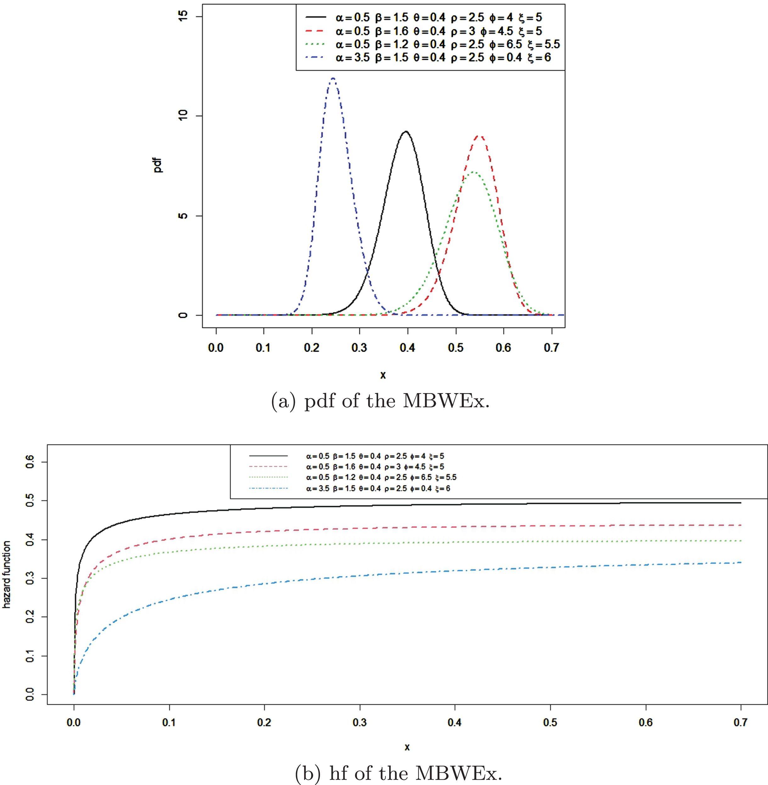
The MBWEx distribution includes the Weibull Exponential(WE) when θ=ζ=φ=1. For θ=α=ρ=1, the MBWEx becomes Beta Exponential(BE) distribution. For θ=ζ=1, MBEx reduces to Exponentiated Weibull Exponential(EWE) distribution. Plots of the density function and the hazard function of the MBWEx with various assigned parameter values are shown in Fig. 1.
Fig. 1
Plots of the Modified Beta Weibull exponential distribution.
2.4Modified Beta Weibull Weibull (MBWW) distribution
The pdf and cdf of Weibull distribution are given as
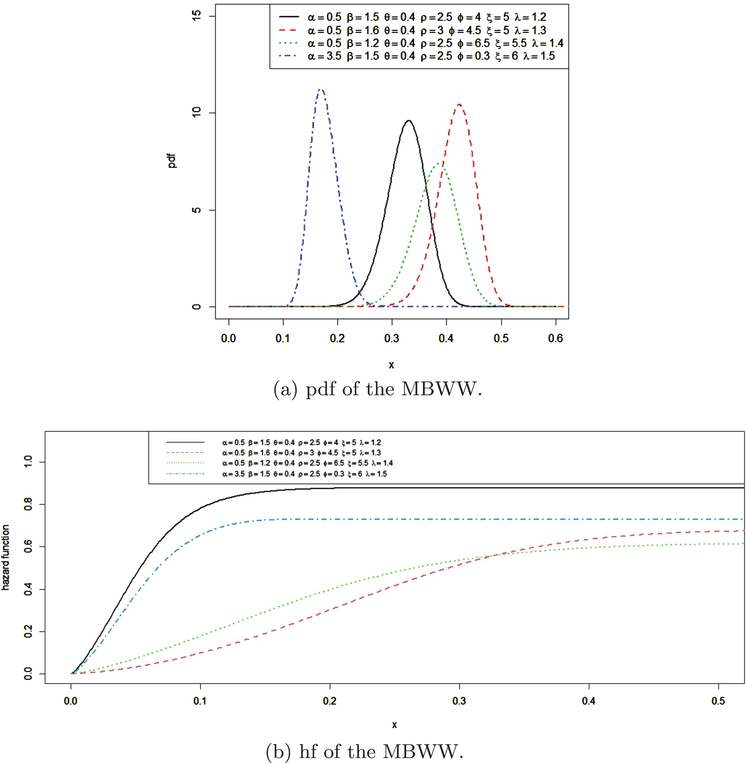
For θ=α=ρ=1, the MBWW becomes Beta Weibull(BW) distribution. For θ=ζ=1, MBWW reduces to Exponentiated Weibull Weibull(EWE) distribution. Plots of the density function and the hazard function of the MBWW with various assigned parameter values are shown in Fig. 2.
Fig. 2
Plots of the Modified Beta Weibull Weibull distribution.
2.5Modified Beta Weibull Frechet (MBWF) distribution
The pdf and cdf of Frechet distribution are given as
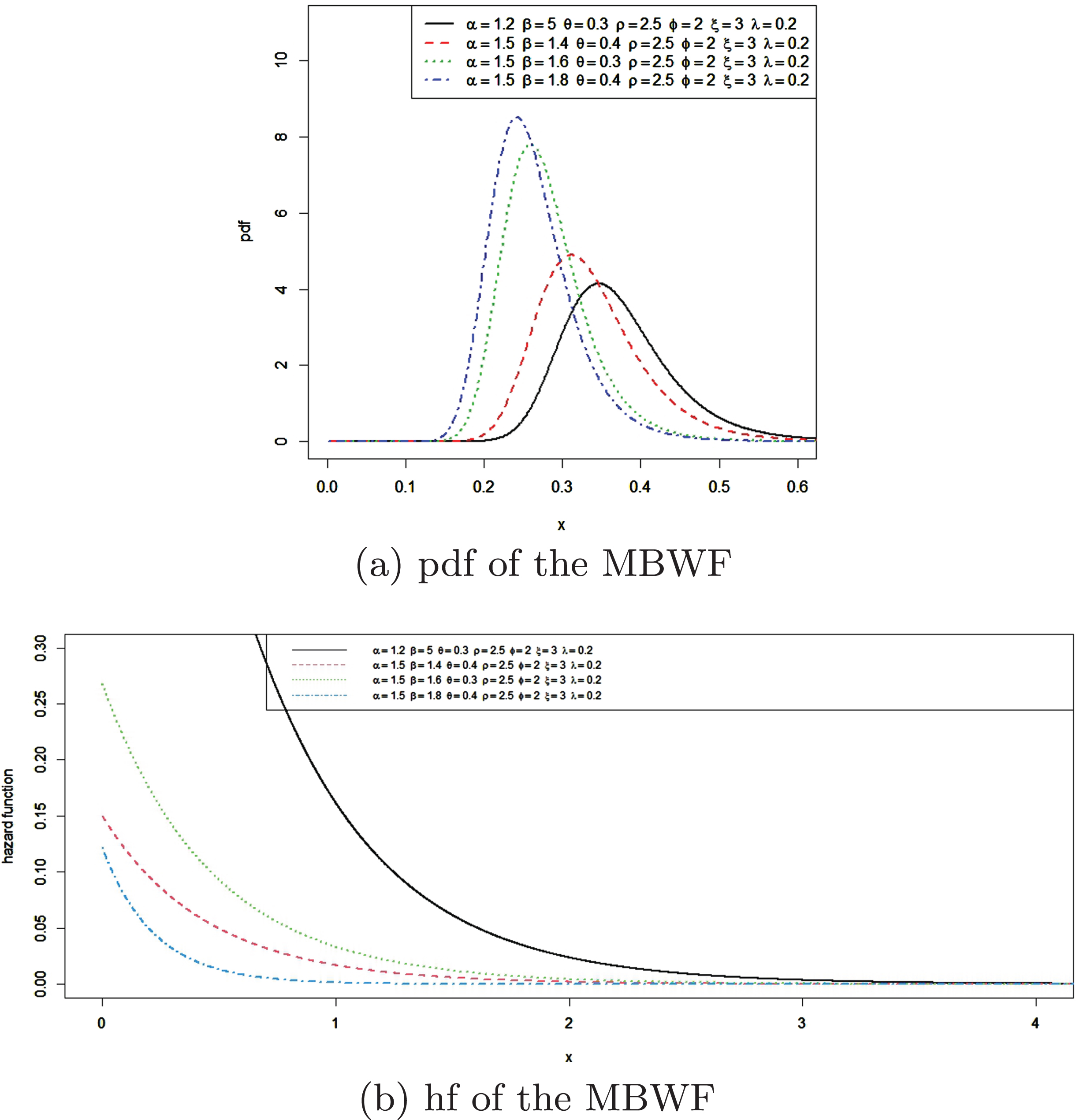
The MBWF distribution includes the Weibull Frechet(WF) when θ=ζ=φ=1. For θ=α=ρ=1, the MBWF becomes Beta Frechet(BF) distribution. For θ=ζ=1. Plots of the density function and the hazard function of the MBWF with various assigned parameter values are shown in Fig. 3.
Fig. 3
Plot of pdf of the Modified Beta Weibull Frechet distribution.
3Linear representation
In this section, a useful mixture representation for the density function of the MBWG distribution is derived. The derived representation is crucial for the derivation of statistical properties of the MBWG distribution such as moments, generating functions, order statistic properties. Using the Binomial Expression given as
(11)
(12)
(13)
(14)
(15)
(16)
(17)
(18)
(19)
(20)
(21)
(22)
(23)
Furthermore, integrating expression in 23, we have the linear mixture c.d.f of the MBWG family in terms of the Exp-G distribution as
(24)
4Statistical properties
In this section, the statistical properties of the MBWG distribution are extensively studied. The properties considered are moments, monet generating function, quantile function, and order statistics
4.1Quantile function
The quantile function of the MBWG distribution is obtained by solving
(25)
4.2Moments
The rth moment
(26)
For the nth central moment of X (Mn), the expression is obtained as
(27)
(28)
(29)
4.3Moment generating function
The moment generating function (Mf (t))= E[etX] of X.In this section, two formula in computing the moment generating function(m.g.f) of the family is discussed.
Firstly, we derived the m.g.f form equation 23 as
Secondly, the m.g.f was also derived from the baseline of the quantile function as
4.4Order statistics
Let X1, . . . , Xn be a random sample from the MBWG distribution, The pdf of ith order statistic, say Xi:n, can be written as
(30)
(31)
5Parameter estimation
In this section, we derived the expressions for the estimates of the parameters of the MBWG distribution. We employed the use of the maximum likelihood estimation (M.L.E) method. Let δ=(ζ,φ,θ,α,ρ,σ) be the parameter vector and x = (x1, . . . . . , xn) be the sample from the MBWG distribution, then the log-likelihood function for δ can be written as
(32)
(33)
(34)
(35)
(36)
(37)
(38)
For interval estimation of the model parameters, we require the observed information matrix for interval estimation and test of hypothesis on the parameters (ζ, φ, θ, α, ρ, θ), we obtain a 6x6 unit information matrix
Under the conditions that are fulfilled for parameters, the asymptotic distribution of
(39)
6Application to real life data sets
In this section, application of the MBWG distribution was done on two real datasets using the Weibull distribution as the baseline model to illustrate the importance and fit of the MBWG distribution. The maximum likelihood estimates (M.L.E) of the distribution and that of the competitive distributions will be obtained. We assessed the goodness of fit of the distributions using the log-likelihood, Akaike’s information criterion (AIC), Bayesian information criterion (BIC), and corrected Akaike’s information criterion (CAIC). The R statistical software is employed for data analysis. Estimation of model parameter estimates was done using the optim() function in stats packages in R version 4.1.1 [32]. The fit of the MBWW distribution is compared with other competitive distributions which are Weibull exponential (WEx) ([30]), Kumaraswamy Weibull (KW) [31]), Beta Weibull (BW) ([28]) and Exponentiated Weibull Weibull (ExWW) ([29]) distributions. The p.d.fs of these distributions are as follows:
• Weibull exponential (WEx) distribution.
• Kumaraswamy Weibull (KW) distribution
• Beta Weibull (BW) distribution
• Exponentiated Weibull Weibull (ExWW) distribution
Data set 1: The first data set represents the breaking strength of 100 yarn as reported by Gomes-Silva et al (2017). The data-set consists of 63 measurements of the strengths of 1.5 cm glass fibres, which were initially collected by United Kingdom National Physical Laboratory staff. The data is presented below:
0.55, 0.74, 0.77, 0.81, 0.84, 1.24, 0.93, 1.04, 1.11, 1.13, 1.30, 1.25, 1.27, 1.28,1.29, 1.48, 1.36, 1.39, 1.42, 1.48, 1.51, 1.49, 1.49, 1.50, 1.50,1.55, 1.52, 1.53, 1.54, 1.55, 1.61, 1.58,1.59, 1.60, 1.61, 1.63,1.61, 1.61, 1.62, 1.62, 1.67, 1.64, 1.66, 1.66, 1.66, 1.70, 1.68,1.68, 1.69, 1.70, 1.78, 1.73, 1.76, 1.76, 1.77, 1.89, 1.81, 1.82,1.84, 1.84, 2.00, 2.01, 2.24.
Data set 2:
The second data set represents the breaking stress of carbon fibers of 50 mm length (GPa) which was reported by Nicholas and Padgett (2006). This data was used by Yousof et al. (2017). The data set is:
0.39, 0.85, 1.08, 1.25, 1.47, 1.57, 1.61, 1.61, 1.69, 1.80, 1.84, 1.87, 1.89, 2.03, 2.03, 2.05, 2.12, 2.35, 2.41, 2.43, 2.48, 2.50, 2.53, 2.55, 2.55, 2.56, 2.59, 2.67, 2.73, 2.74, 2.79, 2.81, 2.82, 2.85, 2.87, 2.88, 2.93, 2.95, 2.96, 2.97, 3.09, 3.11, 3.11, 3.15, 3.15, 3.19, 3.22, 3.22, 3.27, 3.28, 3.31, 3.31, 3.33, 3.39, 3.39, 3.56, 3.60, 3.65, 3.68, 3.70, 3.75, 4.20, 4.38, 4.42, 4.70, 4.90.
After analysis of the two datasets, Fig. 6 describes the shape of the hazard plots of the data. It shows that the hazard curve os non-decreasing for the two datasets. Furthermore Fig. 4 is the histogram which further reveals the fit of the model to both datasets. Figure 5 shows how close the fitted pdf is to the empirical distribution which further established the fact that the model fits the data well. In Tables 1 and 2, we have observed that the modified beta weibull weibull distribution gives the best fit when compared to its submodels, therefore making it the preferred model to consider for this data on the basis of the selection criterion considered.
Fig. 4
Estimated pdf plots for Data I and Data II.
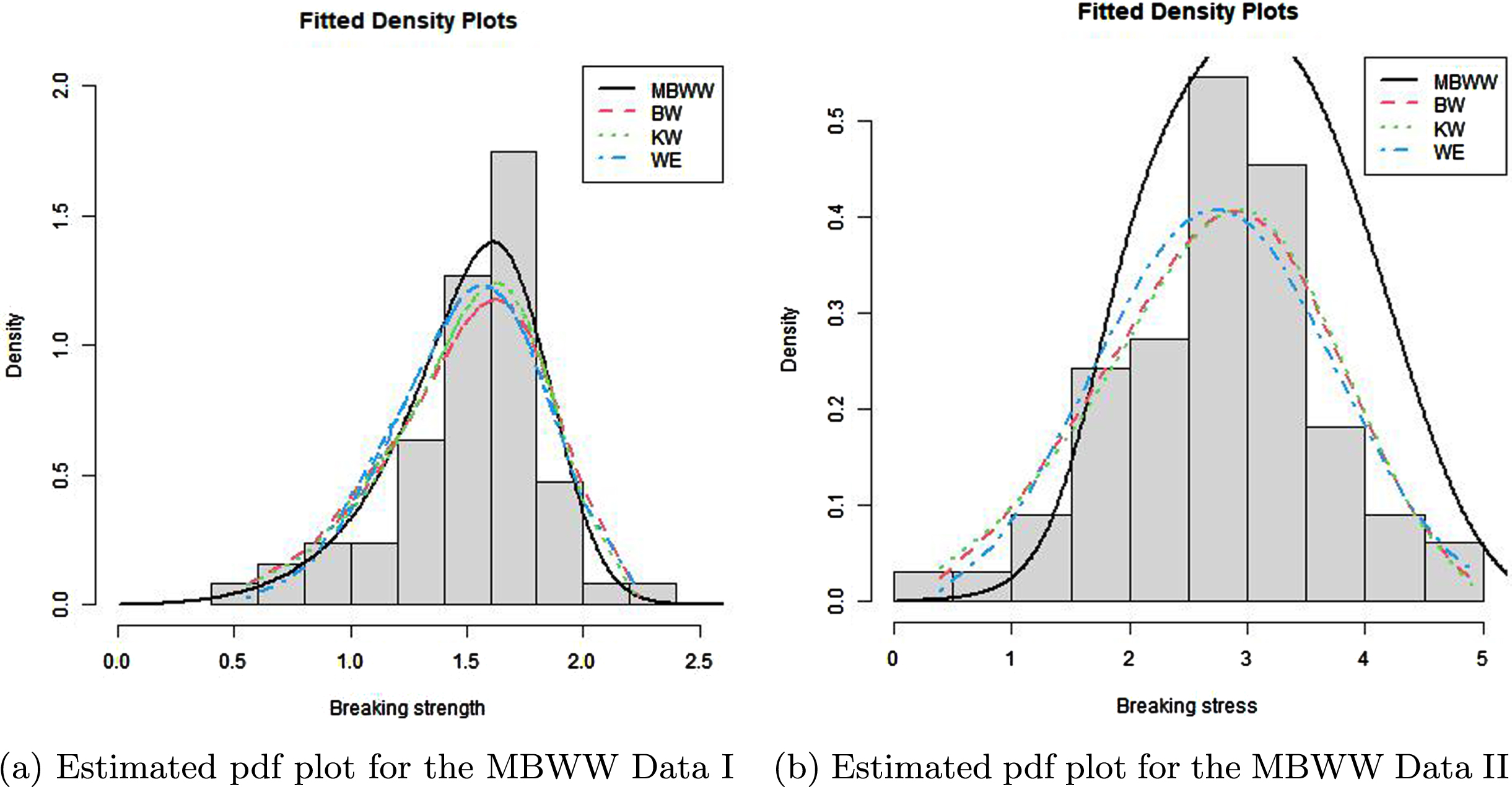
Fig. 5
Estimated cdf plot for the MBWW
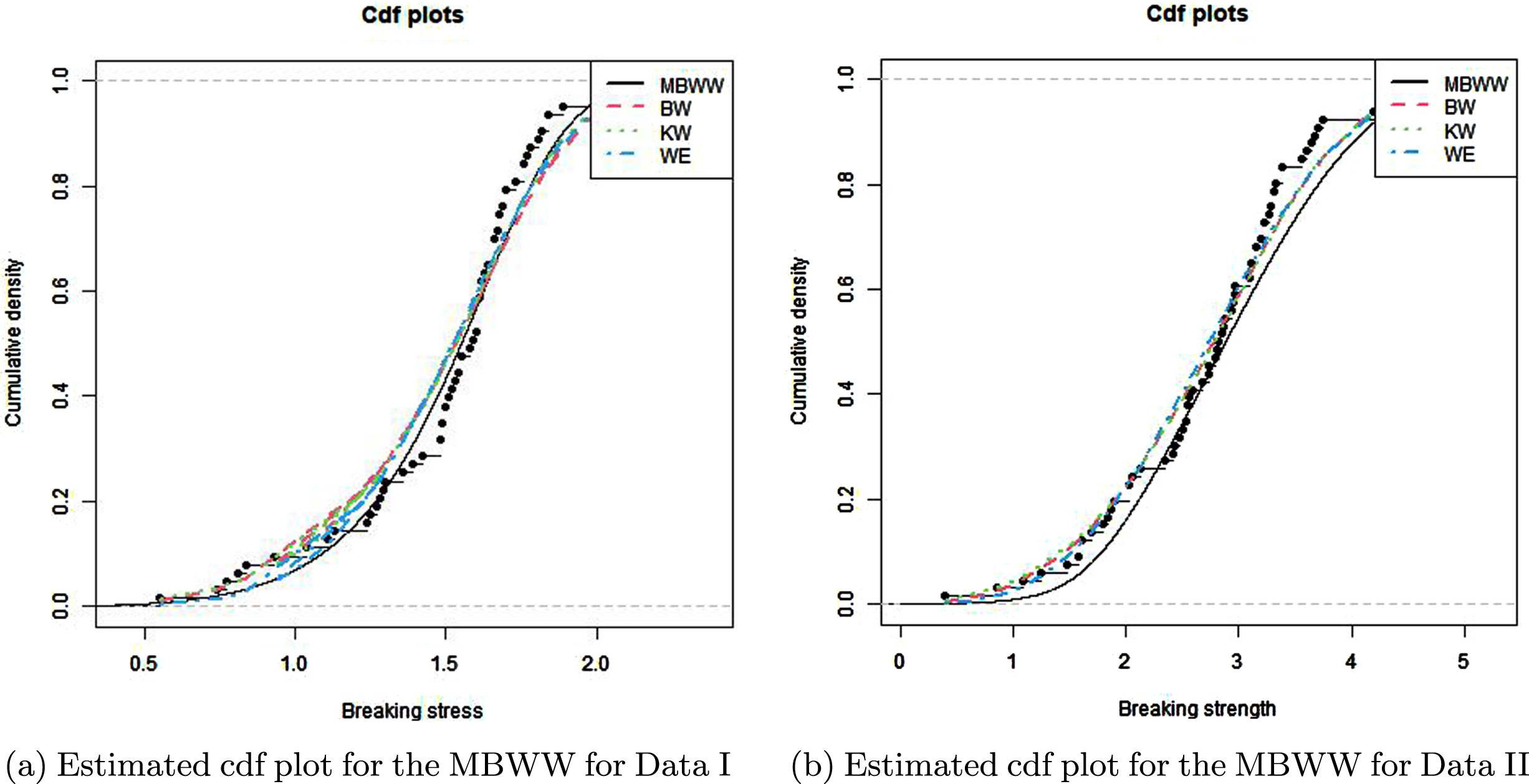
Fig. 6
TTT plot of MBWW
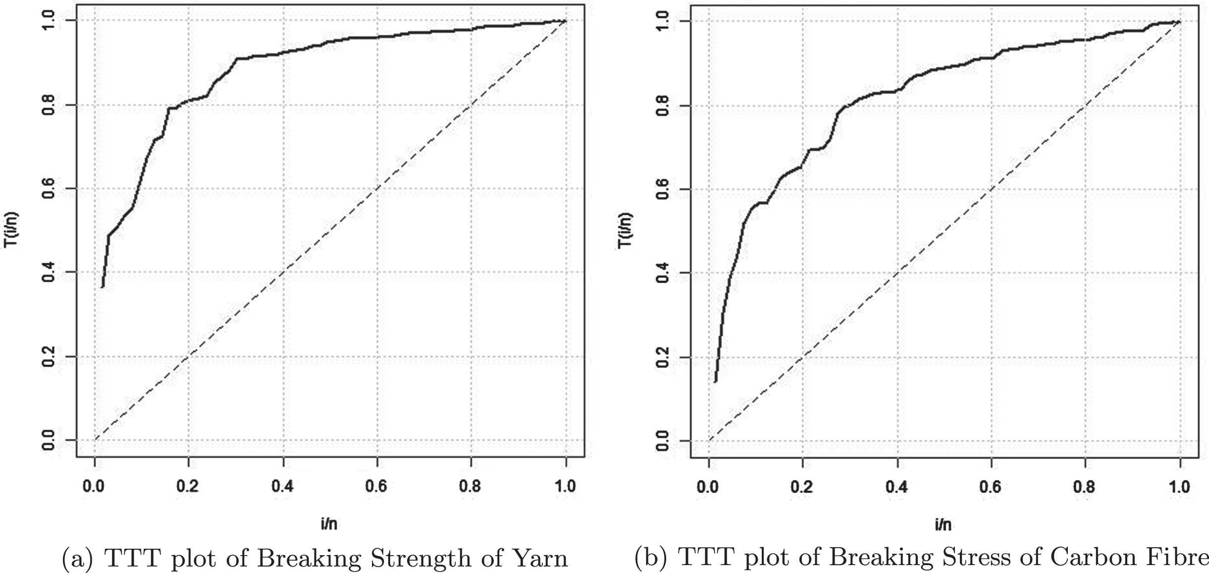
Table 1
The MLEs and Information Criteria of the models based on data set 1
| Model |
|
|
|
|
|
|
| -LL | AIC | BIC | CAIC |
| MBWW | 1.5549 | 0.5758 | 0.7992 | 0.1928 | 2.2280 | 1.4243 | 1.5953 | 11.1390 | 36.2780 | 51.2799 | 38.9446 |
| WEx | 5.3583 | 1.4233 | 0.8726 | - | - | - | - | 15.5250 | 37.0500 | 43.4794 | 37.45684 |
| KW | 0.5040 | 0.1729 | 6.5245 | 1.2858 | - | - | - | 15.0980 | 38.1959 | 46.7685 | 38.8856 |
| BW | 0.6243 | 6.4974 | 7.1824 | 2.3007 | - | - | - | 14.6656 | 37.3311 | 45.9036 | 38.3837 |
| EKW | 1.8536 | 5.5418 | 0.4837 | 5.0944 | 2.0662 | - | - | 14.8422 | 39.6844 | 50.4001 | 40.7371 |
Table 2
The MLEs and Information Criteria of the models based on data set 2
| Model |
|
|
|
|
|
|
| -LL | AIC | BIC | CAIC |
| MBWW | 0.6931 | 0.0250 | 1.4581 | 1.2725 | 0.7170 | 0.0823 | 1.5192 | 67.2027 | 148.4056 | 153.345 | 149.708 |
| WEx | 3.2187 | 1.4841 | 0.4835 | - | - | - | - | 86.3347 | 178.6695 | 185.2385 | 179.0566 |
| KW | 0.5380 | 0.1338 | 3.6983 | 1.8507 | - | - | - | 86.3365 | 180.6732 | 189.4318 | 181.3289 |
| BW | 0.7280 | 4.5270 | 3.9104 | 4.9847 | - | - | - | 86.1975 | 180.3951 | 189.1537 | 181.0508 |
| EKW | 0.0673 | 0.1641 | 2.9947 | 2.8437 | 1.4215 | - | - | 85.0870 | 180.1732 | 191.1214 | 181.1732 |
7Conclusion
In applications to real life situations, there has always been a clear need for extended forms of existing distributions which are more flexible and gives better fit to model real data which has high degree of kurtosis and skewness. In this work, we proposed a new family of distribution called the Modified Beta Weibull Family which generalizes the beta weibull G family by the addition of a shape parameter. Some well known family of distributions are special cases of the Modified Beta Weibull Family. Some mathematical properties of the new class including linear expression of the distribution,,moments,quantile, moment generating functions and order statistics are provided. The model parameters are estimated by the maximum likelihood estimation method and the observed information matrix is determined. We prove empirically by means of an application to a real data set that special cases of the proposed family can give better fits than other models generated from well-known families.
References
[1] | Abouelmagd T. , Hamed M. , Ebraheim H. , The Poisson-G Family of Distributions with Applications.? Pakistan Journal of Statistics and Operation Research 13: ((2017) ), 313. doi: 10.18187/pjsor.v13i2.1740. |
[2] | Afify A. , Yousof H.M. , Nadarajah S. , The beta transmuted-H family for lifetime data.? Statistics and Its Interface 10: ((2017) ), 505–520. doi: 10.4310/SII.2017.v10.n3.a13. |
[3] | Afify A. , Yousof H.M. , Cordeiro G. , Ortega E. , Nofal Z. , The Weibull Fréchet Distribution and its Applications, Journal of Applied Statistics 43: ((2016) ), 2608–2626. 10.1080/02664763.2016.1142945. |
[4] | Oguntunde P.E. , Balogun O.S. , Okagbue H.I. , Bishop S.A. , The Weibull-Exponential Distribution: Its Properties and Applications, Journal of Applied Sciences 15: ((2015) ), 1305–1311. |
[5] | Klakattawi H.S. , The Weibull-Gamma Distribution: Properties and Applications, Entropy ((2019) ), 21. |
[6] | Ibrahim N.A. , Khaleel M.A. , Merovci F. , Kílíçman A. and Shitan N., Weibull Burr X distribution properties and application, ((2017) ). |
[7] | Awodutire P. , Statistical Properties and Applications of the Exponentiated Chen-G Family of Distributions: Exponential Distribution as a Baseline Distribution, Austrian Journal of Statistics 51: (2) ((2022) ), 57–90. |
[8] | Awodutire P.O. , Nduka E.C. , Ijomah M.A. , The Beta Type I Generalized Half Logistic Distribution: Properties and Application, Asian Journal of Probability and Statistics 6: (2) ((2020) ), 27–41. https://doi.org/10.9734/ajpas/2020/v6i230156. |
[9] | Bourguignon M. , Silva R. , GM C. , The Weibull-G family of probability distributions, J. Data Sci. 12: (2014), 53. |
[10] | Cordeiro G. , Alizadeh M. , Tahir M. , Mansoor M. , Bourguignon M. , Hamedani G. , The Beta Odd Log-Logistic Generalized Family of Distributions, Hacettepe University Bulletin of Natural Sciences and Engineering Series B: Mathematics and Statistics 45: ((2015) ). 10.15672/HJMS.20157311545. |
[11] | Cordeiro G.M. , Afify A.Z. , Yousof H.M. , Pescim R.R. , Aryal G.R. , Mediterranean Journal of Mathematics 14: ((2017) ), Article number: 155. |
[12] | Elbatal I. , Jamal F. , Chesneau C. , Elgarhy M. , The Modified Beta Gompertz Distribution:Theory and Applications.? Mathematics ((2018) ), 7. doi: 10.3390/math7010003. |
[13] | Elgarhy M. , Shakil M. , Kibria B.M. , Exponentiated Weibull-Exponential Distribution with Applications, Applications and Applied Mathematics: An International Journal (AAM) 12: ((2017) ), 710–725. |
[14] | Eugene N. , Lee C. , Famoye F. , Beta-normal distribution and its applications, Commun. Stat.-Theory Methods 31: ((2002) ), 497. |
[15] | Famoye F. , Lee C. , Olumolade O. , The beta-Weibull distribution, Journal of Statistical Theory and Applications 4: ((2005) ), 121–136. |
[16] | Gupta R. , Gupta P. , Gupta R. , Modeling failure time data by Lehmann alternatives, Commun. Stat. Theory Methods 27: ((1998) ), 887. |
[17] | Hassan A. , Elgarhy M. , Exponentiated Weibull-Weibull Distribution: Statistical Properties and Applications, Gazi University Journal of Science ((2018) ). |
[18] | Hussain Z. , Asghar Z. , Cubic Transmuted-G Family of Distributions and Its Properties, Stochastics and Quality Control 33: ((2018) ). doi: 10.1515/eqc-2017-0027. |
[19] | Jose J. , Manoharan M. , Beta half logistic distribution: A new probability model for lifetime data, Journal of Statistics and Management Systems 19: ((2016) ), 587–604. 10.1080/09720510.2015.1103457. |
[20] | Klakattawi H.S. , The Weibull-sigma Distribution: Properties and Applications, Entropy 19. |
[21] | Makubate B. , Oluyede B. , Motobetso G. , Huang S. , Fagbamigbe A. , The Beta Weibull-G Family of Distributions: Model, Properties and Application, International Journal of Statistics and Probability 7: ((2018) ), 12. 10.5539/ijsp.v7n2p12. |
[22] | Nadarajah S. , Gupta A. , The beta Fréchet distribution, Far East Journal of Theoretical Statistics 14: ((2004) ). |
[23] | Nadarajah S. , Kotz S. , The beta exponential distribution, Reliability Engineering and System Safety 91: (6) ((2006) ), 689–697. |
[24] | Nadarajah S. , Teimouri M. , Shih S. , Modified Beta Distributions. Sankhya:, The Indian Journal of Statistics 76: ((2014) ), 19–48. doi: 10.1007/s13571-013-0077-0. |
[25] | Saboor A. , Khan M.N. , Cordeiro G.M. , Pascoa M.A. , Bortolini J. , Mubeen S. , Modified beta modified-Weibull distribution, Comput Stat 34: ((2019) ), 173–199. https://doi.org/10.1007/s00180-018-0822-y |
[26] | Shaw W.T. , Buckley I.R. , The alchemy of probability distributions: Beyond GramCharlier expansions, and a skew-kurtotic-normal distribution from a rank transmutation map, ((2009) ). |
[27] | Gradshteyn I.S. , Ryzhik I.M. , Table of Integrals, Series, and Products, seventh edition, Academic Press, New York. (2007) MR2360010 map. |
[28] | Famoye F. , Lee C. , Olumolade O. , The beta-Weibull distribution, Journal of Statistical Theory and Applications 4: ((2005) ), 121–136. |
[29] | Hassan A. , Elgarhy M. , Exponentiated Weibull-Weibull Distribution: Statistical Properties and Applications, Gazi University Journal of Science 32: (2) ((2018) ), 616–635. |
[30] | Oguntunde P. , Balogun O. , Okagbue H. , Amina B. , The Weibull-Exponential Distribution: Its Properties and Applications, Journal of Applied Fire Science 15: ((2015) ), 1305–1311. |
[31] | Cordeiro Gauss M., Edwin M.M. and Nadarajah S., The Kumaraswamy Weibull distribution with application to failure data, Journal of the Franklin Institute 347: (8) ((2010) ), 1399–1429. |
[32] | R Core Team. R: A language and environment for statistical computing. R Foundation for Statistical Computing, Vienna, Austria. ((2020) ) URL https://www.R-project.org/. |


