
A novel transfer deep learning model with reinforcement-learning-based hyperparameter optimization for short-term load forecasting during the COVID-19 pandemic
Abstract
The coronavirus disease 2019 pandemic has significantly impacted the world. The sudden decline in electricity load demand caused by strict social distancing restrictions has made it difficult for traditional models to forecast the load demand during the pandemic. Therefore, in this study, a novel transfer deep learning model with reinforcement-learning-based hyperparameter optimization is proposed for short-term load forecasting during the pandemic. First, a knowledge base containing mobility data is constructed, which can reflect the changes in visitor volume in different regions and buildings based on mobile services. Therefore, the sudden decline in load can be analyzed according to the socioeconomic behavior changes during the pandemic. Furthermore, a new transfer deep learning model is proposed to address the problem of limited mobility data associated with the pandemic. Moreover, reinforcement learning is employed to optimize the hyperparameters of the proposed model automatically, which avoids the manual adjustment of the hyperparameters, thereby maximizing the forecasting accuracy. To enhance the hyperparameter optimization efficiency of the reinforcement-learning agents, a new advance forecasting method is proposed to forecast the state-action values of the state space that have not been traversed. The experimental results on 12 real-world datasets covering different countries and cities demonstrate that the proposed model achieves high forecasting accuracy during the coronavirus disease 2019 pandemic.
1Introduction
Short-term load forecasting (STLF) refers to the load forecasting from one hour to one week [1]. Forecasted short-term load facilitates efficient dispatching of power systems. Although STLF is challenging owing to the significant uncertainty and volatility of the load demand, it has been well handled by some deep learning models, such as convolutional neural networks (CNNs) [2], long short-term memory networks (LSTMs), and recurrent neural networks (RNNs) [3]. In our previous work [4], an ensemble deep learning model with dynamic error correction method and multi-objective ensemble pruning method was proposed for time series forecasting.
However, the coronavirus disease 2019 (COVID-19) pandemic has severely impacted the daily lives of people worldwide. Relevant policies have been promulgated in many countries and regions, requiring people to obey strict social distancing restrictions because of the high infectiousness of COVID-19. Traditional deep learning models for STLF generally use previous load demand, timing information, and weather data as input features [5]. However, it is difficult for deep learning models to capture the sudden decline in load demand during the pandemic caused by strict social distancing restrictions, because the social and economic information produced by the COVID-19 pandemic is often neglected. It is therefore difficult to achieve the balance between electricity generation and load demand because of the inaccurate load forecasting results, which may lead to large-scale blackouts.
The mobility data provided by Google1 and Apple2 reflect the changes in visitor volume in different regions and buildings based on mobile services, which are location specific and aggregated across the population [6]. Le Quéré et al. [7] demonstrated that there is a strong correlation between the mobility data and economic activities. Therefore, a knowledge base comprising mobility data is conducive to improving the forecasting accuracy of the STLF models during the pandemic. However, it is difficult for traditional deep learning models to exploit the knowledge base efficiently because of the limited mobility data associated with the pandemic.
Transfer learning is an approach that utilizes the knowledge accumulated from data in the source domain to solve forecasting problems in the target domain involving different data patterns [8]. The transfer deep learning model can adequately utilize the knowledge base with limited mobility data by combining the data utilization ability of transfer learning with the nonlinear fitting ability of deep learning. However, it is computationally expensive to adjust the hyperparameters of transfer deep learning models to maximize the forecasting accuracy. To the best of our knowledge, there is no effective hyperparameter optimization method for the transfer deep learning models.
Reinforcement learning is an artificial intelligence technology that seeks an optimal strategy and maximizes benefits through continuous interactions with the environment [9]. Reinforcement learning has been widely used to solve diverse optimization problems. However, no research has been reported to optimize the hyperparameters of transfer deep learning models using reinforcement learning algorithms, because it is difficult for the reinforcement-learning agents to completely traverse the large state space composed of different hyperparameters.
To bridge the above research gap and inspired by Chen et al. [6], a novel transfer deep learning model with reinforcement-learning-based hyperparameter optimization and advance forecasting method (TDL-RLHO-AFM) is proposed for STLF during the COVID-19 pandemic. The main contributions of this study are summarized as follows:
(1) A knowledge base comprising mobility data is constructed. The socioeconomic behavior changes can be leveraged to analyze the sudden decline in the load during the pandemic, hence improving the load forecasting accuracy during the pandemic.
(2) A new transfer deep learning model (TDL) is proposed to solve the problem of limited mobility data associated with the pandemic, which efficiently utilizes the socioeconomic behavior changes across different geographical regions. It also inspires a new insight for load forecasting during some other public emergencies.
(3) A new reinforcement-learning-based hyperparameter optimization (RLHO) method is proposed to optimize the hyperparameters of the proposed model automatically and maximize the forecasting accuracy of the proposed model by transforming the hyperparameter optimization problem into a Markov decision process (MDP).
(4) A new advance forecasting method (AFM) is proposed to forecast the state-action values of the state space that has not been traversed, which handles the difficulty for the reinforcement-learning agents to completely traverse the large state space comprising different hyperparameters and enhances the hyperparameter optimization efficiency of reinforcement-learning agents.
(5) A total of 12 real-world datasets covering different countries and cities are used to verify the effectiveness of the proposed model. The experimental results demonstrate that the proposed model achieves high forecasting accuracy during the COVID-19 pandemic.
The remainder of this paper is organized as follows. Section 2 provides a review of previous research on the STLF problem, transfer learning, and reinforcement learning. Section 3 introduces the construction of the knowledge base. Section 4 presents the proposed TDL-RLHO-AFM model in detail. Section 5 describes the implementation details and experimental results of TDL-RLHO-AFM on 12 datasets. Section 6 outlines the conclusions and discusses the future work.
2Related work
This section briefly presents previous research on the STLF problem, transfer learning, and reinforcement learning.
2.1Short-term load forecasting
Short-term load forecasting models can be categorized into persistence, physical, statistical, and artificial intelligence models [10]. Deep learning models, which belong to artificial intelligence models, are good at STLF, owing to their excellent nonlinear fitting ability on different features, including previous load demand, timing information, and weather data. For example, Qiu et al. [11] proposed a hybrid incremental learning approach for STLF, which was composed of random vector functional link network, discrete wavelet transformation, and empirical mode decomposition. Avatefipour and Nafisian [12] proposed a method based on clonal selection algorithm and artificial neural network for STLF, which used fuzzy set theory to select the most informative and irredundant features from the input feature set. Kim et al. [13] proposed a deep learning model for STLF, which combined RNN and CNN to calibrate the hidden state vector values obtained from different features. Motepe et al. [14] used long short-term memory recurrent neural network to forecast the power consumption of large South African power users, which considered the impact of temperature. Afrasiabi et al. [10] proposed an end-to-end model comprising of CNN and gated recurrent unit for residential load forecasting by utilizing the load consumption information of residents and the meteorological data. Chitalia et al. [15] presented an RNN model to forecast the short-term load in different types of commercial buildings by utilizing the features of different building types and locations. Peng et al. [16] proposed a hybrid RNN model for STLF, which could select the spatial and temporal features that were most relevant to the load demand. However, it is difficult for these deep learning models to forecast the load demand with traditional features during the COVID-19 pandemic because of the massive impact of the pandemic on the power system.
The COVID-19 pandemic has been detected in more than 200 countries, resulting in tens of millions of confirmed cases and hundreds of thousands of deaths worldwide in 2020. The strict social distancing restrictions used to deal with the high infectiousness of COVID-19 have altered load demand tremendously. For example, the average load demand of the New York Independent System Operator (NYISO) area in March fell by 9% than that in the previous year, which was reduced from 17102 watt to 15640 watt [17]. The load demand of New York in April of 2020 was 21% lower than that in the previous year. In Italy, the largest reduction in the observed load demand was 25% [18]. Therefore, the socioeconomic behavior changes associated with the pandemic need to be analyzed to capture the sudden decline in load demand caused by strict social distancing restrictions.
The mobility data provided by Apple and Google reflect the changes in visitor volume in different regions and buildings, which also reflect the socioeconomic behavior changes during the pandemic. In this study, a knowledge base comprising mobility data is constructed for STLF during the pandemic so that the socioeconomic behavior changes can be leveraged to analyze the sudden decline in load during the pandemic. However, only small parts of mobility data are associated with the pandemic, making it difficult for deep learning models to exploit the socioeconomic behavior changes adequately.
To solve the aforementioned problem, a novel TDL model is proposed, which can efficiently utilize the socioeconomic behavior changes by sharing the mobility data across different geographical regions.
2.2Transfer learning
Transfer learning was first introduced in 1996 [19]; however, it did not attract widespread attention until 2018. Transfer learning does not require training and testing data to follow the same distribution [20]. Therefore, it can solve the problem of limited training data by reusing the data from other different but related domains. For example, Laptev et al. [21] proposed a transfer learning model for time series forecasting, which used transfer learning to alleviate the plight of limited training data. Ribeiro et al. [22] proposed a transfer learning model for cross-building energy forecasting, which merged the data from similar buildings with different distributions and solved the problem of small historical datasets. Cai et al. [23] proposed a two-layer transfer-learning-based model for STLF, which solved the problem of limited load data in the target zone. Gupta et al. [24] proposed a transfer learning model for clinical time series forecasting to solve the problem of limited clinically labeled data. Jung et al. [25] proposed a model based on transfer learning to forecast the monthly electric load in cities, by selecting the similar data from other cities to satisfy the required amount of data for model training. Fong et al. [26] combined the transfer learning with RNN to forecast the concentration levels of air pollutants, which solved the problem of limited observed data in air quality monitoring stations. Lee and Rhee [27] adopted transfer learning and meta learning for load forecasting, by taking full advantage of the limited residential dataset collected over just several days.
There are limited mobility data associated with the pandemic, which make it difficult for traditional deep learning models to forecast the load during the pandemic. Inspired by the above studies, a new TDL model is proposed herein to solve the problem of limited mobility data associated with the pandemic. However, the forecasting accuracy is heavily influenced by the hyperparameter optimization of TDL models, which was not considered in the above studies. It is also computationally expensive to optimize the hyperparameters of TDL models to maximize the forecasting accuracy. Therefore, a new RLHO method is proposed in this study to automatically optimize the hyperparameters of the proposed model.
2.3Reinforcement learning
Reinforcement learning obtains the optimal solution to a specific problem by modeling the problem as an MDP and allowing the agents to continuously interact with the environment. The reinforcement learning models, including Q-learning [28] and state-action-reward-state-action [29], have achieved considerable contributions in the fields of optimization and decision-making. For example, Brandi et al. [30] proposed a reinforcement learning model to control the supply water temperature setpoint of a heating system and obtained promising results for an office building in an integrated simulation environment. Zou et al. [31] used reinforcement learning to solve the dynamic multi-objective optimization problem, which was proven to be effective through the evaluation on a real-world problem.
In recent years, reinforcement learning has gradually been used in the field of hyperparameter optimization, which can efficiently avoid deceptive local optima and handle the high-dimensional parameter vector [32]. For example, Meng et al. [33] used reinforcement learning to optimize the weighting parameters of a dynamic priority scheduling algorithm. Bu et al. [32] proposed a reinforcement learning method to optimize a large number of hyperparameters of a composite load model with distributed generation.
However, reinforcement-learning agents have difficulty in completely traversing the large state space comprising different hyperparameters, resulting in local optimal hyperparameters. In this study, an RLHO combined with a new AFM is proposed to forecast the state-action values of the state space that has not been traversed, which can enhance the hyperparameter optimization efficiency of reinforcement-learning agents.
3Construction of knowledge base
The knowledge base constructed in this study includes four types of normalized data: load data, time index, weather data, and mobility data. It covers 12 different geographical regions, including the United Kingdom (UK), Germany, France, the California Independent System Operator (CAISO) area, the NYISO area, Dallas, Houston, San Antonio (SA), Boston, Chicago, Philadelphia, and Seattle. The acquired data range from February 15, 2020 to May 15, 2020, covering the period before and after the policy of strict social distancing restrictions was promulgated to tackle the pandemic.
(1) The load data represent the hourly load demand in different geographical regions. The load data of European regions are obtained from the European Network of Transmission System Operators, and the load data of the United States are obtained from the respective independent system operators in the United States.
(2) The time index represents the day of the week and hour information through the One-Hot code [34].
(3) The weather data are obtained from World Weather Online, which contain the information on cloud coverage, humidity, precipitation, pressure, and temperature.
(4) The mobility data are obtained from Google and Apple, revealing the relative changes in visitor volume in different regions and buildings. The mobility data obtained from Google reveal the relative changes in visitor volume at six different locations: retail and recreation, grocery and pharmacy, parks, transit stations, workplaces, and residential areas. The baseline volumes are the median of the 5-week period from January 3, 2020 to February 6, 2020. The mobility data obtained from Apple reveal the relative changes in visitor volume for three types of movements: driving, transit, and walking. The baseline volumes are the data on January 13, 2020. Google and Apple collect the information based on the location history of the users’ accounts [6]. Take the mobility data at 10 o’clock on March 1, 2020 in Boston as an illustrative example, and the specific values are shown in Table 1.
Table 1
The values of mobility data provided by Google and Apple
| Different locations or movements | Percentage of change from baseline |
| Retail and recreation | 55.29 |
| Grocery and pharmacy | 20.99 |
| Parks | 52.26 |
| Transit stations | –58 |
| Workplaces | –16 |
| Residential areas | 21 |
| Driving | –70 |
| Transit | –46 |
| Walking | 15 |
As shown in Table 1, the visitor volumes at retail and recreation, grocery and pharmacy, parks, and residential areas are increased by 55.29%, 20.99%, 52.26%, and 21%, respectively. The other values can be self-explainable similarly.
4Methodology
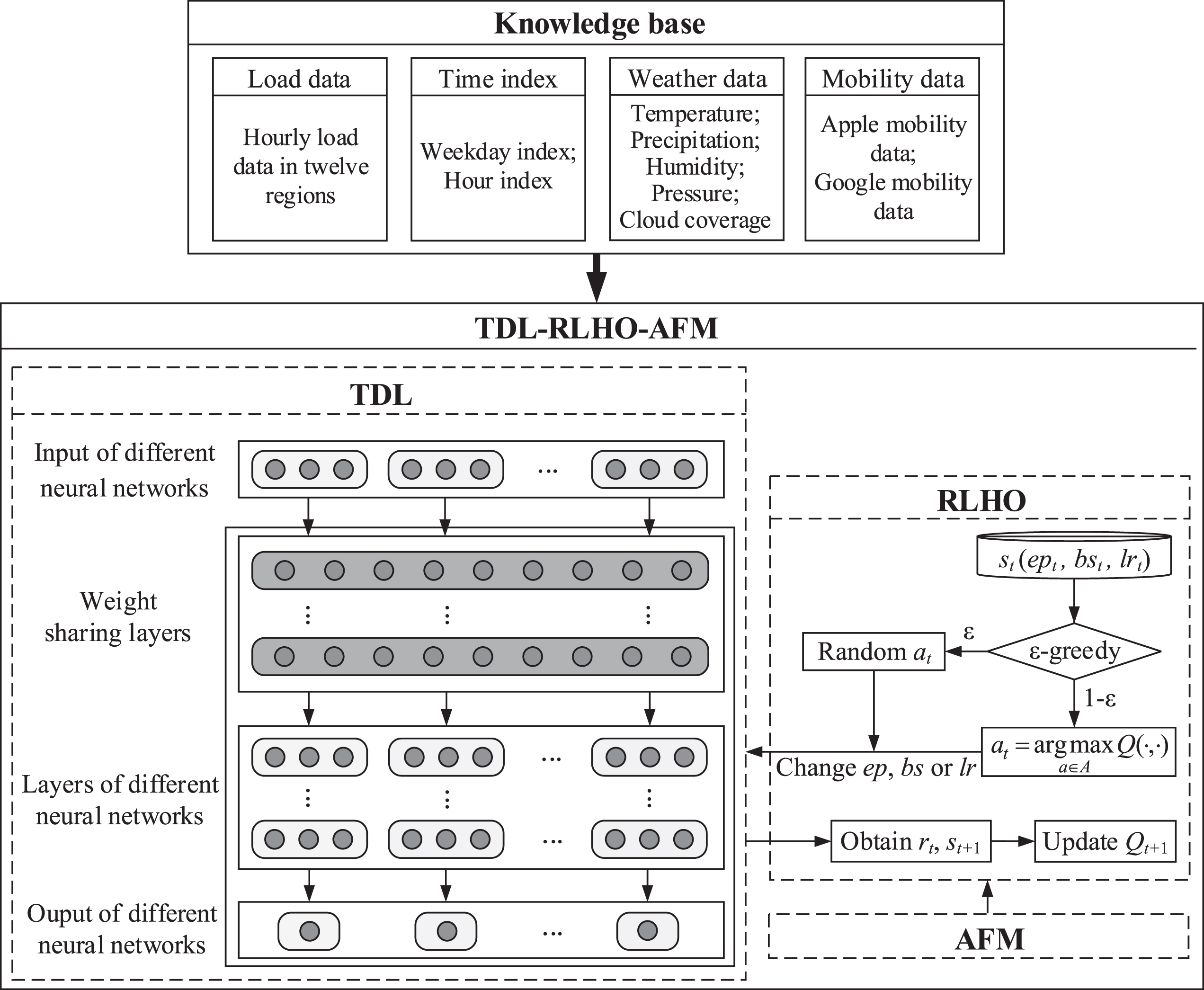
The proposed TDL-RLHO-AFM model consists of three parts: a TDL model, an RLHO method, and an AFM. The RLHO method is used to optimize the hyperparameters of neural networks in different layers, which are contained in TDL model. The AFM is used to enhance the hyperparameter optimization efficiency of RLHO method and obtain the better hyperparameters. The framework diagram of the proposed TDL-RLHO-AFM model is shown in Fig. 1 and is detailed in the following sub-sections.
Fig. 1
Overview of TDL-RLHO-AFM
4.1Transfer deep learning model
In this study, a new TDL model is proposed to solve the problem of limited mobility data associated with the pandemic, which uses the transfer knowledge learned from source domains to solve other target learning tasks. The data covering different source domains include time index, weather data, and mobility data of different geographical regions, and the different learning tasks refer to the STLF in different geographical regions. The definition of TDL is shown as follows.
Definition of transfer deep learning: Given a source domain DS, a source learning task TS, a target domain DT, and a target learning task TT, the TDL model will improve the learning ability of the target forecasting function rT (·) in DT using the transfer knowledge learned from DS and TS, where DS≠DT, and TS≠TT.
According to the definition above, each domain of transfer deep learning is defined as a pair D = {F, P (X)}, where F = {f1, …, fn} is a feature space with n dimensions. X = {x1, …, xn} ∈ F is the learning sample, and P(X) is the marginal probability distribution of X [22]. The feature space and marginal probability distributions differ across different domains. Each learning task is defined as a pair T = {y, r (·)}, where y is the value space of the true load demand, and r(·) is the forecasting function. Referring to Fig. 1, the TDL model includes the following steps:
(1) First, the data from different source domains are used as the input of the neural networks for solving different learning tasks.
(2) Second, the transfer knowledge is transformed into the weight sharing layers of the proposed model, which can be utilized by all learning tasks. In this study, all weight sharing layers are constructed based on RNN, and the hyperparameters of each weight sharing layer are set to be the same.
(3) Finally, the neural networks for different learning tasks are trained, and the forecasting results are output respectively.
4.2Reinforcement-learning-based hyperparameter optimization method
Reinforcement learning models the problem as an MDP, through which, the agents interact with the environment through trial and error over discrete time steps [9]. The goal of the agents is to select an action that maximizes the expected discount reward. In this study, the hyperparameters of the proposed TDL model are optimized through a reinforcement learning method, so as to improve the forecasting accuracy. MDPs are generally defined as < S, A, P, R > [36]:
• S refers to the set of all possible valid states of the agents, including the different values of epoch, batch size, and learning rate in the proposed TDL model. s refers to the specific state, where ∀s ∈ S.
• A refers to the set of all possible valid actions of agents. At each time point, the agents take one of the six potential actions and change the value of the epoch, batch size, or learning rate accordingly. a refers to a specific action, where ∀a ∈ A.
• P refers to the transition probability distribution of the agents in the constructed environment.
• R is the reward function of the agents,
Q π (s, a) is defined as the state-action value, which means the expected cumulative discount reward obtained by executing action a under state s following policy π: S⟶A, as shown in Equation (1) [36]:
(1)
The Q-learning algorithm [38] is used in this study to continuously estimate the optimal state-action value through the Bellman equation to obtain the optimal policy
(2)
The pseudocode of the RLHO method for the TDL model is shown in Algorithm 1, where Q(·,·) refers to the set of state-action values at all time points, and the value of Qt+1 (st, at) is the Q value at time point t + 1. An episode with different number of time steps is one complete play of the agents interacting with the environment in the general reinforcement learning setting [41].
Algorithm 1
| RLHO method | |
| 1: | Input: number of episodes M, number of time steps T, discount factor γ, hyperparameter ɛ, value of epoch ep, value of batch size bs, and value of learning rate lr |
| 2: | Initialize Q0 (s0, a0) for s in S and a in A, initialize ep0, bs0, and lr0 randomly, and set Q (·, ·) =0 |
| 3: | for episode = 1, . . . ,M do |
| 4: | Receive initial state s1 |
| 5: | for t = 1, . . . , T do |
| 6: | if a random number> ɛ then |
| 7: | Select at= argmax(Q(·,·)) |
| 8: | else |
| 9: | Select at randomly where at∈ |
| 15: | Update s ← st+1 |
| 16: | end for |
| 17: | end for |
Figure 1 and Algorithm 1 show the main process of the RLHO method, which can be described as follows:
(1) At each time point, obtain the action at through the ɛ-greedy algorithm. at is an integer, with different values representing different actions, as listed in Table 2.
(2) Run the TDL model with the current values of epoch, batch size, and learning rate at time point t. Then, the forecasting accuracy of the TDL model at time point t is obtained, which is presented by means of the mean absolute percentage error (MAPE) [42] as Equation (3):
where N indicates the number of forecasting hours, and yi and pi are the actual and forecasted values of the ith hour, respectively.(3)
(3) Obtain the reward rt at time point t and execute the action at to get the new state st+1, which includes the new values of epoch, batch size, and learning rate at time point t + 1.
(4) Update the Q value and the state at time point t + 1, repeat the above procedures until the termination time step is reached.
(5) Select the corresponding state with the largest Q value of all time points, representing the optimized hyperparameters.
Table 2
The values of at and their corresponding actions
| The value of at | Corresponding actions |
| 0 | Add 1 to the value of epoch |
| 1 | Subtract 1 from the value of epoch |
| 2 | Add 1 to the value of batch size |
| 3 | Subtract 1 from the value of batch size |
| 4 | Add 0.0001 to the value of learning rate |
| 5 | Subtract 0.0001 from the value of learning rate |
4.3Advance forecasting method
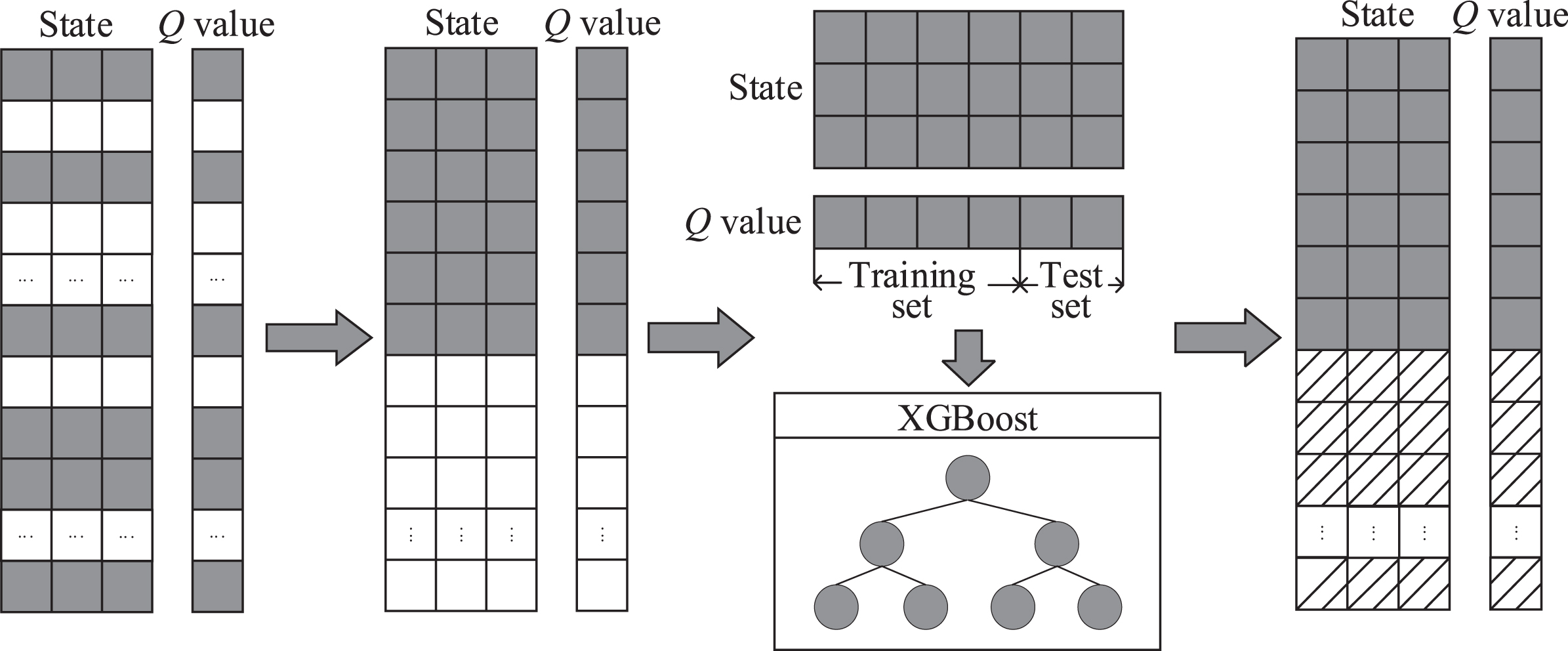
The hyperparameters obtained through Q-learning are usually sub-optimal because of the large state space. In this study, an AFM is proposed to forecast the corresponding Q values of the states that have not been traversed at some time points by means of the extreme gradient boosting (XGBoost) [43] algorithm, which is a widely recognized machine learning method. AFM enhances the hyperparameter optimization efficiency of reinforcement-learning agents and obtains the better hyperparameters.
The AFM process is described as follows (Fig. 2). Each Q value represents the state-action value of the state that has or has not been traversed by the agents at different time points.
(1) First, in the proposed TDL model with the RLHO method, a part of states are traversed by the agents, with the corresponding Q values obtained. The gray squares in Fig. 2 represent the states that have been traversed by the agents, together with their corresponding Q values. The white squares represent the states that have not been traversed by the agents, together with their corresponding Q values.
(2) Second, the states that have been traversed by the agents with their corresponding Q values are divided into the training set and test set, which are used to train the XGBoost.
(3) Finally, the trained XGBoost model is used to forecast the Q values of states that have not been traversed by the agents, which are represented by the squares with oblique lines in Fig. 2. Then, the corresponding state with the largest Q value is selected, representing the near optimal hyperparameters.
Fig. 2
Overview of AFM.
5Experiments and analysis
This section shows the experimental implementation details, presents the results of different comparison experiments, and analyzes the experimental results.
5.1Experimental platforms and parameters
The experimental platforms in this study are described in Table 3.
Table 3
Hardware and software platforms
| Hardware and software platform | Configuration |
| Operating system | Windows 10 |
| RAM | 32 GB |
| CPU | Intel Core i7-8700K |
| GPU | GeForce RTX 2080 |
| Programing language | Python |
| Deep learning software library | Keras |
| Integrated development environment | Spyder |
In this study, the sequence length of the input is 24, and the day-ahead load demand are forecasted. The forecasting accuracy of different models is represented by the MAPE. The smaller values of MAPE indicate the more accurate forecasting results. The data are normalized according to Equation (4) [44], and some other data pre-processing techniques, such as outlier detection technique [45], are also used in this study.
(4)
All experimental results of the models in this study are obtained by averaging the forecasting results through five runs. The training set of the experiments in this study covers the period from February 15, 2020 to April 30, 2020, and the test set covers the period from May 1, 2020 to May 14, 2020. The proposed TDL-RLHO-AFM model is constructed based on the RNN, and the default hyperparameters are listed in Table 4.
Table 4
Experimental hyperparameters of different algorithms
| Algorithm | Experimental hyperparameter | Value |
| TDL | Step size of learning rate | 0.0001 |
| Step size of batch size | 1 | |
| Step size of epoch | 1 | |
| RLHO | ɛ of ɛ-greedy | 0.3 |
| Decay rate of ɛ | 0.99 | |
| Reward discount rate | 0.95 | |
| Learning rate | 0.1 | |
| AFM | Number of iterations | 160 |
| Learning rate | 0.1 | |
| Maximum depth of tree | 3 | |
| RNN/CNN/LSTM | Learning rate | 0.0001 |
| Number of epochs | 50 | |
| Batch size | 32 | |
| Activation function | relu |
5.2Experiments results and discussions
5.2.1Performance of mobility data
This sub-section verifies the effect of the constructed knowledge base containing the mobility data. The forecasting results of the RNN with knowledge base (RNN_KB) and RNN without knowledge base (RNN) are shown in Table 5. The significant values are boldfaced.
Table 5
Comparison of the forecasting results of RNN with knowledge base and RNN without knowledge base
| Dataset | France | Germany | UK | NYISO | CAISO | Dallas | Houston | SA | Boston | Chicago | Philadelphia | Seattle |
| RNN | 0.1199 | 0.1049 | 0.2442 | 0.1175 | 0.0966 | 0.0974 | 0.1079 | 0.1066 | 0.1045 | 0.1260 | 0.2029 | 0.1144 |
| RNN_KB | 0.0714 | 0.0533 | 0.2137 | 0.0412 | 0.0411 | 0.0885 | 0.0714 | 0.1063 | 0.0434 | 0.0370 | 0.0506 | 0.0500 |
Note: Significant values are boldfaced.
As shown in Table 5, the forecasting accuracy of the RNN with knowledge base is higher than that of the RNN without knowledge base. For France, Germany, UK, NYISO, CAISO, Dallas, Houston, SA, Boston, Chicago, Philadelphia, and Seattle, the forecasting accuracy is improved by 40.5%, 49.2%, 12.5%, 64.9%, 57.5%, 9.1%, 33.8%, 0.2%, 58.5%, 70.6%, 75.1%, and 56.3%, respectively. The experiments in this sub-section demonstrate that the knowledge base, in particular, its contained mobility data, can improve the forecasting accuracy of deep learning model during the pandemic.
5.2.2Performance of transfer deep learning
This sub-section verifies the effect of the TDL model. The forecasting results of the TDL and the RNN without transfer learning (RNN_KB) are shown in Table 6, and the significant values are boldfaced. Note that the forecasting results of RNN_KB are different from the results in Table 5 because the averaging results are obtained through five runs again.
Table 6
Comparison of the forecasting results between TDL model and RNN without transfer learning
| Dataset | France | Germany | UK | NYISO | CAISO | Dallas | Houston | SA | Boston | Chicago | Philadelphia | Seattle |
| RNN_KB | 0.0669 | 0.0529 | 0.1905 | 0.0402 | 0.0413 | 0.0906 | 0.0690 | 0.1002 | 0.0451 | 0.0365 | 0.0517 | 0.0540 |
| TDL | 0.0663 | 0.0521 | 0.1715 | 0.0418 | 0.0468 | 0.0867 | 0.0676 | 0.1079 | 0.0413 | 0.0372 | 0.0448 | 0.0494 |
Note: Significant values are boldfaced.
As shown in Table 6, compared with the RNN without transfer learning, the TDL model has higher forecasting accuracy on eight datasets (i.e., France, Germany, UK, Dallas, Houston, Boston, Philadelphia, and Seattle), and it has lower forecasting accuracy on only four datasets (i.e., NYISO, CAISO, SA, and Chicago). Generally, the TDL model outperforms the RNN without transfer learning because the TDL model can take advantage of the socioeconomic behavior changes contained in the mobility data, demonstrating the effectiveness of transfer learning during the pandemic.
5.2.3Performance of reinforcement-learning-based hyperparameter optimization with advance forecasting method
This sub-section verifies the effect of RLHO and AFM. The value scopes of different hyperparameters in this sub-section are shown in Table 7.
Table 7
Value scopes of different hyperparameters
| Hyperparameter | Scope |
| Epoch | [0, 30] |
| Batch size | [30, 60] |
| Learning rate | [0, 0.005] |
The forecasting results of the proposed TDL-RLHO-AFM model with different episodes and time steps are presented in Table 8. Different combinations of episodes and time steps represent the number of states that can be traversed by the agents. For example, the combination of 5 episodes and 10 time steps means that the agents can traverse up to 50 states. Variables ep, bs, and lr represent the best values of epoch, batch size, and learning rate of the proposed model with different episodes and time steps, respectively. State_num represents the number of states that have been traversed by the agents. Time represents the time cost of training the proposed model with different episodes and time steps. MAPE represents the forecasting accuracy of the proposed model. The significant values of MAPE on all datasets are boldfaced.
Table 8
The forecasting results of the proposed model with different episodes and time steps
| Dataset | Episode×step | ep | bs | lr | State_num | Time(s) | MAPE |
| France | 5×10 | 30 | 34 | 0.0011 | 38 | 2074 | 0.0661 |
| 10×30 | 21 | 54 | 0.0008 | 227 | 14792 | 0.0595 | |
| 30×30 | 11 | 56 | 0.0012 | 608 | 39765 | 0.0566 | |
| 10×100 | 30 | 45 | 0.0005 | 447 | 47750 | 0.0605 | |
| Germany | 5×10 | 2 | 44 | 0.0012 | 40 | 1820 | 0.0519 |
| 10×30 | 9 | 56 | 0.0010 | 211 | 14141 | 0.0488 | |
| 30×30 | 16 | 37 | 0.0004 | 589 | 37230 | 0.0476 | |
| 10×100 | 7 | 31 | 0.0005 | 455 | 54219 | 0.0450 | |
| UK | 5×10 | 15 | 52 | 0.0017 | 45 | 2450 | 0.1308 |
| 10×30 | 26 | 51 | 0.0025 | 212 | 12589 | 0.1358 | |
| 30×30 | 27 | 44 | 0.0025 | 577 | 38126 | 0.1306 | |
| 10×100 | 29 | 53 | 0.0014 | 518 | 64011 | 0.1266 | |
| NYISO | 5×10 | 16 | 41 | 0.0003 | 47 | 2804 | 0.0342 |
| 10×30 | 23 | 59 | 0.0009 | 209 | 15749 | 0.0327 | |
| 30×30 | 30 | 44 | 0.0005 | 581 | 44860 | 0.0315 | |
| 10×100 | 20 | 37 | 0.0002 | 492 | 68059 | 0.0318 | |
| CAISO | 5×10 | 29 | 30 | 0.0043 | 36 | 2004 | 0.0438 |
| 10×30 | 13 | 40 | 0.0020 | 190 | 12231 | 0.0405 | |
| 30×30 | 15 | 56 | 0.0001 | 620 | 38160 | 0.0367 | |
| 10×100 | 27 | 57 | 0.0002 | 440 | 47489 | 0.0387 | |
| Dallas | 5×10 | 15 | 41 | 0.0034 | 43 | 2297 | 0.0346 |
| 10×30 | 7 | 48 | 0.0009 | 191 | 13949 | 0.0332 | |
| 30×30 | 15 | 50 | 0.0008 | 610 | 49426 | 0.0308 | |
| 10×100 | 29 | 41 | 0.0011 | 500 | 69528 | 0.0324 | |
| Houston | 5×10 | 20 | 32 | 0.0017 | 34 | 1616 | 0.0358 |
| 10×30 | 7 | 30 | 0.0004 | 199 | 11547 | 0.0316 | |
| 30×30 | 17 | 33 | 0.0001 | 615 | 42138 | 0.0323 | |
| 10×100 | 29 | 59 | 0.0017 | 445 | 43195 | 0.0315 | |
| SA | 5×10 | 13 | 42 | 0.0013 | 46 | 2353 | 0.0319 |
| 10×30 | 18 | 53 | 0.0001 | 168 | 10078 | 0.0325 | |
| 30×30 | 25 | 41 | 0.0003 | 666 | 45353 | 0.0313 | |
| 10×100 | 20 | 52 | 0.0017 | 394 | 38220 | 0.0332 | |
| Boston | 5×10 | 15 | 34 | 0.0010 | 36 | 1768 | 0.0339 |
| 10×30 | 29 | 33 | 0.0016 | 186 | 11700 | 0.0330 | |
| 30×30 | 18 | 45 | 0.0005 | 574 | 34590 | 0.0328 | |
| 10×100 | 30 | 39 | 0.0006 | 516 | 68292 | 0.0339 | |
| Chicago | 5×10 | 23 | 32 | 0.0002 | 41 | 2360 | 0.0345 |
| 10×30 | 30 | 49 | 0.0006 | 186 | 12980 | 0.0317 | |
| 30×30 | 3 | 38 | 0.0002 | 632 | 41322 | 0.0306 | |
| 10×100 | 30 | 31 | 0.0011 | 514 | 66050 | 0.0320 | |
| Philadelphia | 5×10 | 11 | 49 | 0.0004 | 35 | 1775 | 0.0338 |
| 10×30 | 24 | 48 | 0.0004 | 190 | 10485 | 0.0313 | |
| 30×30 | 5 | 33 | 0.0009 | 575 | 34096 | 0.0316 | |
| 10×100 | 30 | 45 | 0.0001 | 467 | 54719 | 0.0338 | |
| Seattle | 5×10 | 13 | 47 | 0.0021 | 33 | 1744 | 0.0371 |
| 10×30 | 11 | 41 | 0.0007 | 200 | 13237 | 0.0333 | |
| 30×30 | 1 | 42 | 0.0010 | 610 | 37413 | 0.0310 | |
| 10×100 | 5 | 50 | 0.0014 | 515 | 58982 | 0.0321 |
According to the experimental results shown in both Table 6 and Table 8, the following results can be obtained:
(1) Referring to both Tables 6 and 8, the forecasting accuracy of the proposed TDL-RLHO-AFM model is higher than that of TDL, which is improved by 14.6%, 13.6%, 26.2%, 24.6%, 21.6%, 64.5%, 53.4%, 71.0%, 20.1%, 17.7%, 30.1%, and 37.2% on the datasets of France, Germany, UK, NYISO, CAISO, Dallas, Houston, SA, Boston, Chicago, Philadelphia, and Seattle, respectively. The results demonstrate the effectiveness of reinforcement learning for optimizing hyperparameters.
(2) Referring to Table 8, in 8 of the 12 datasets, the forecasting accuracy of the proposed model with 30 episodes and 30 time steps is higher than that of the proposed model with 10 episodes and 100 steps, indicating that the better hyperparameters are found by the agents in the proposed model with 30 episodes and 30 time steps. This also shows that the agents traversing more states do not always find the better hyperparameters because they may encounter the boundary of the state space more often.
(3) Referring to Table 8, the use of AFM significantly enhances the hyperparameter optimization efficiency of the reinforcement-learning agents. For example, on the France dataset, when the episode is 30 and the time step is 30, the agents can traverse up to 900 (30×30) states. However, the agents actually spend 39,765 seconds (i.e., 11.05 hours) to traverse 608 states and obtain the corresponding Q values, because the Q values of the remaining 292 (900–608) states are forecasted using AFM. Because these 292 states are not actually traversed, the time cost of 19,097 (292/608*39,765) seconds (i.e., 5.30 hours) are saved.
Table 9 and Fig. 3 present the forecasting accuracies and forecasting results of the proposed model corresponding to different hyperparameter combinations from May 1, 2020 to May 14, 2020 on the NYISO dataset. The significant values of MAPE are boldfaced. The legends of Fig. 3 indicate the different hyperparameter combinations. For example, (30, 30, 0.0001) means the epoch is 30, the batch size is 30, and the learning rate is 0.0001. The unit of load data is megawatt (MW) in Fig. 3.
Table 9
The forecasting accuracies of the proposed model with different hyperparameter combinations
| Different hyperparameter combinations | MAPE | ||
| Epoch | Batch size | Learning rate | |
| 0 | 30 | 0.0001 | 0.0391 |
| 0 | 30 | 0.005 | 0.0835 |
| 0 | 60 | 0.0001 | 0.0385 |
| 0 | 60 | 0.005 | 0.0755 |
| 30 | 30 | 0.0001 | 0.0392 |
| 30 | 30 | 0.005 | 0.0561 |
| 30 | 60 | 0.0001 | 0.0366 |
| 30 | 60 | 0.005 | 0.0545 |
| 30 | 44 | 0.0005 | 0.0315 |
Note: Significant values are boldfaced.
Fig. 3
Comparison of forecasting results of the proposed model with different hyperparameter combinations.
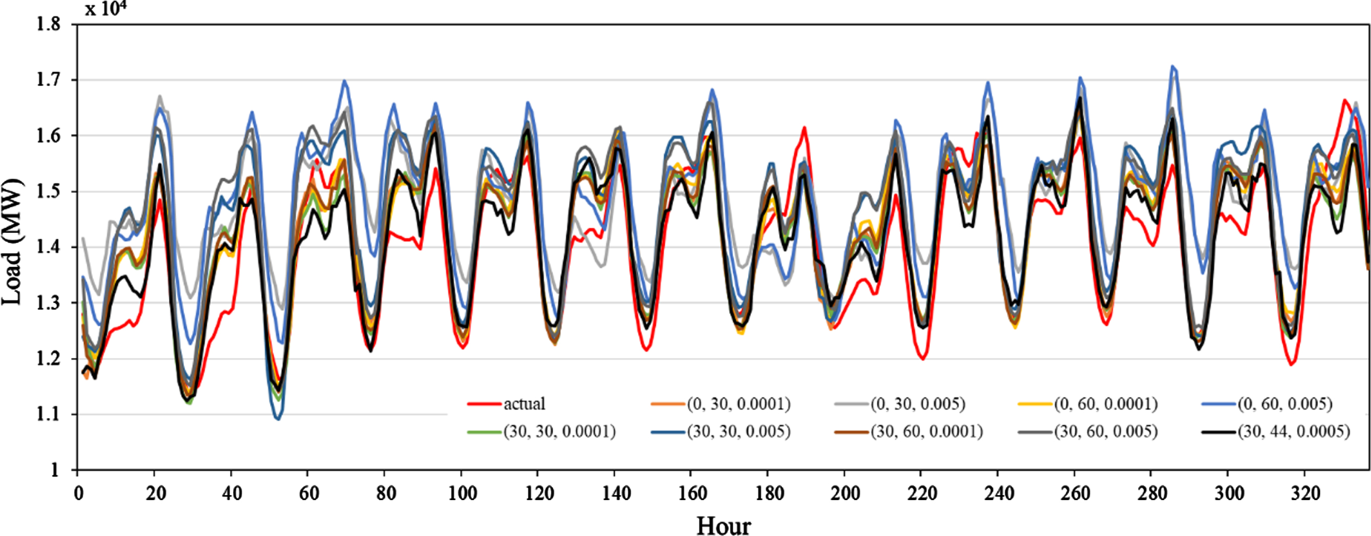
As shown in Table 9 and Fig. 3, different hyperparameter values have great influence on the forecasting results of the model, and they are not linearly correlated. The proposed model with the hyperparameters values found by reinforcement learning has the best forecasting accuracy, demonstrating the effectiveness of reinforcement learning.
In order to verify the effect of the proposed model further, CNN and LSTM are used for comparison due to their good ability of feature learning. The forecasting accuracies of the proposed model, CNN and LSTM with knowledge base (CNN_KB and LSTM_KB), and CNN and LSTM without knowledge base (CNN and LSTM) are shown in Table 10. The significant values of MAPE are boldfaced.
Table 10
Comparison of the forecasting accuracies of the proposed model and other methods
| Dataset | France | Germany | UK | NYISO | CAISO | Dallas | Houston | SA | Boston | Chicago | Philadelphia | Seattle |
| CNN | 0.1447 | 0.1204 | 0.2260 | 0.1910 | 0.1342 | 0.1157 | 0.1016 | 0.1086 | 0.1289 | 0.1283 | 0.1705 | 0.1354 |
| CNN_KB | 0.0811 | 0.0789 | 0.2152 | 0.0379 | 0.0601 | 0.0840 | 0.0958 | 0.1230 | 0.0418 | 0.0456 | 0.0598 | 0.0716 |
| LSTM | 0.2451 | 0.1219 | 0.2253 | 0.2178 | 0.0891 | 0.2240 | 0.1154 | 0.1338 | 0.2497 | 0.1868 | 0.2380 | 0.1607 |
| LSTM_KB | 0.1300 | 0.1369 | 0.2131 | 0.0812 | 0.0738 | 0.1175 | 0.0812 | 0.1171 | 0.1131 | 0.0906 | 0.0955 | 0.1342 |
| Proposed model | 0.0566 | 0.0450 | 0.1266 | 0.0315 | 0.0367 | 0.0308 | 0.0315 | 0.0313 | 0.0328 | 0.0306 | 0.0313 | 0.0310 |
Note: Significant values are boldfaced.
As shown in Table 10, the forecasting accuracy of the proposed TDL-RLHO-AFM model is higher than that of the CNN and LSTM either with or without knowledge base. The experiments in this sub-section demonstrate the effectiveness of the proposed model for load forecasting during the pandemic.
Figure 4 shows the line chart of forecasting results of the proposed TDL-RLHO-AFM model, CNN and LSTM with knowledge base (CNN_KB and LSTM_KB), and CNN and LSTM without knowledge base (CNN and LSTM) from May 1, 2020 to May 14, 2020 on the NYISO dataset. The unit of the load data is megawatt (MW).
Fig. 4
Comparison of forecasting results of the proposed model and other methods.
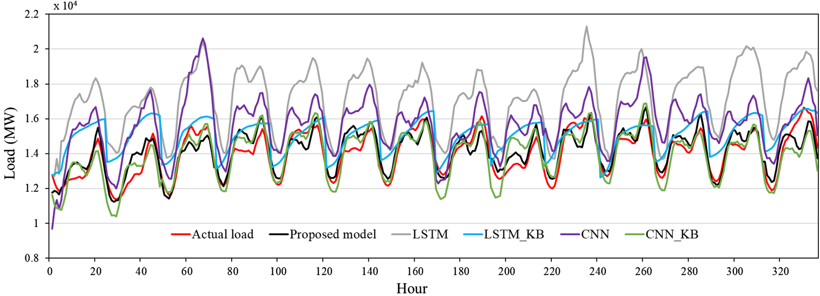
As shown in Fig. 4, the forecasting results of the proposed TDL-RLHO-AFM model are closer to the actual loads than other methods, visually illustrating the effectiveness of the proposed model for load forecasting during the pandemic.
6Conclusions and future work
In this study, a novel TDL model with RLHO and AFM is proposed for STLF during the COVID-19 pandemic. Twelve real-world datasets covering different countries and cities are used to verify the performance of the proposed model. Based on the results of multiple comparison experiments, the following four conclusions are summarized as follows:
(1) The socioeconomic behavior changes contained in the knowledge base are beneficial for deep learning models to forecast sudden load decline during the pandemic. It also provides a new direction for load forecasting under other global emergencies.
(2) The proposed TDL model can overcome the problem of limited mobility data associated with the pandemic by making full use of the socioeconomic behavior changes in the knowledge base.
(3) The proposed RLHO method can automatically optimize the hyperparameters of the TDL model.
(4) The proposed AFM can improve the hyperparameter optimization efficiency of the reinforcement-learning agents by forecasting the state-action values of the states that have not been traversed.
Although the proposed model has achieved high forecasting accuracy during the pandemic, it also has some limitations. First, the agents may reach the boundary of the state space, which increases lots of unnecessary time costs, and necessitates a more effective reinforcement learning algorithm that can improve the search efficiency of the agents. Second, generative adversarial networks can expand the limited mobility data [46], therefore, the effectiveness of this technique can be explored in the future work. Finally, various variables affect the forecasting accuracy of deep learning models [47]. However, the study did not explore the influence of various variables except mobility data on load forecasting, which will be considered in the future work.
Conflicts of interest
The authors declare that there is no conflict of interest regarding the publication of this article.
Acknowledgments
The work has been supported by National Natural Science Foundation of China (No. 51875503, No. 51975512), Zhejiang Natural Science Foundation of China (No. LZ20E050001), Zhejiang Key R & D Project of China (No.2021C03153).
References
[1] | Mocanu E. , Nguyen P.H. , Gibescu M. and Kling W.L. , Deep learning for estimating building energy consumption, Sustainable Energy, Grids and Networks 6: ((2016) ), 91–99. |
[2] | Ferreira A. and Giraldi G. , Convolutional neural network approaches to granite tiles classification, Expert Systems with Applications 84: ((2017) ), 1–11. |
[3] | Kim T.Y. and Cho S.B. , Predicting residential energy consumption using CNN-LSTM neural networks, Energy 182: ((2019) ), 72–81. |
[4] | Zhang S. , Chen Y. , Zhang W.Y. and Feng R.J. , A novel ensemble deep learning model with dynamic error correction and multi-objective ensemble pruning for time series forecasting, Information Sciences 544: ((2021) ), 427–445. |
[5] | Chen K.J. , Chen K.L. , Wang Q. , He Z.Y. , Hu J. and He J.J. , Short-term load forecasting with deep residual networks, IEEE Transactions on Smart Grid 10: (4) ((2018) ), 3943–3952. |
[6] | Chen Y.Z. , Yang W.W. and Zhang B.S. , Using mobility for electrical load forecasting during the covid-19 pandemic, arXiv preprint arXiv:2006.08826, (2020). |
[7] | Le Quéré C. , Jackson R.B. , Jones M.W. , Smith A.J. , Abernethy S. , Andrew R.M. , et al., Temporary reduction in daily global CO2 emissions during the COVID-19 forced confinement, Nature Climate Change 10: (7) ((2020) ), 647–653. |
[8] | Lu J. , Behbood V. , Hao P. , Zuo H. , Xue S. and Zhang G.Q. , Transfer learning using computational intelligence: A survey, Knowledge-Based Systems 80: ((2015) ), 14–23. |
[9] | Sutton R.S. and Barto A.G. , Reinforcement Learning: An Introduction, Massachusetts: The MIT Press, ((2018) ). |
[10] | Afrasiabi M. , Mohammadi M. , Rastegar M. , Stankovic L. , Afrasiabi S. and Khazaei M. , Deep-based conditional probability density function forecasting of residential loads, IEEE Transactions on Smart Grid 11: (4) ((2020) ), 3646–3657. |
[11] | Qiu X.H. , Suganthan P.N. and Amaratunga G.A. , Ensemble incremental learning random vector functional link network for short-term electric load forecasting, Knowledge-Based Systems 145: ((2018) ), 182–196. |
[12] | Avatefipour O. and Nafisian A. , A novel electric load consumption prediction and feature selection model based on modified clonal selection algorithm, Journal of Intelligent & Fuzzy Systems 34: (4) ((2018) ), 2261–2272. |
[13] | Kim J. , Moon J. , Hwang E. and Kang P. , Recurrent inception convolution neural network for multi short-term load forecasting, Energy and Buildings 194: ((2019) ), 328–341. |
[14] | Motepe S. , Hasan A.N. , Twala B. and Stopforth R. , Effective load forecasting for large power consuming industrial customers using long short-term memory recurrent neural networks, Journal of Intelligent & Fuzzy Systems 37: (6) ((2019) ), 8219–8235. |
[15] | Chitalia G. , Pipattanasomporn M. , Garg V. and Rahman S. , Robust short-term electrical load forecasting framework for commercial buildings using deep recurrent neural networks, Applied Energy 278: ((2020) ), 115410. |
[16] | Peng J.Y. , Wang D.K. , Kimmig A. , Langovoy M.A. , Wang J.H. and Ovtcharova J. , A hybrid RNN model for mid-to-long term electricity demand forecasting incorporating weather influences, AT-Automatisierungstechnik 69: (1) ((2021) ), 73–83. |
[17] | Paaso A. , Bahramirad S. , Beerten J. , Bernabeu E. , Chiu B. , Enayati B. , et al., Sharing knowledge on electrical energy Industry’s first response to COVID-19, Retrieved December 17 from, 2020. https://resourcecenter.ieee-pes.org/technical-publications/white-paper/PES_TP_COVID19_20.html |
[18] | International Energy Agency (IEA). Covid-19 impact on electricity, Retrieved December 17, 2020, from https://www.iea.org/reports/covid-19-impact-on-electricity |
[19] | Pratt L. and Jennings B. , A survey of transfer between connectionist networks, Connection Science 8: (2) ((1996) ), 163–184. |
[20] | Ye R. and Dai Q. , A novel transfer learning framework for time series forecasting, Knowledge-Based Systems 156: ((2018) ), 74–99. |
[21] | Laptev N. , Yu J. and Rajagopal R. , Reconstruction and regression loss for time-series transfer learning, Special Interest Group on Knowledge Discovery and Data Mining (SIGKDD) and Workshop on the Mining and Learning from Time Series (MiLeTS), London, UK, ((2018) , August). |
[22] | Ribeiro M. , Grolinger K. , ElYamany H.F. , Higashino W.A. and Capretz M.A. , Transfer learning with seasonal and trend adjustment for cross-building energy forecasting, Energy and Buildings 165: ((2018) ), 352–363. |
[23] | Cai L. , Gu J. and Jin Z.J. , Two-layer transfer-learning-based architecture for short-term load forecasting, IEEE Transactions on Industrial Informatics 16: (3) ((2019) ), 1722–1732. |
[24] | Gupta P. , Malhotra P. , Narwariya J. , Vig L. and Shroff G. , Transfer learning for clinical time series analysis using deep neural networks, Journal of Healthcare Informatics Research 4: (2) ((2020) ), 112–137. |
[25] | Jung S.M. , Park S. , Jung S.W. and Hwang E. , Monthly electric load forecasting using transfer learning for smart cities, Sustainability 12: (16) ((2020) ), 6364. |
[26] | Fong I.H. , Li T.Y. , Fong S. , Wong R.K. and Tallon-Ballesteros A.J. , Predicting concentration levels of air pollutants by transfer learning and recurrent neural network, Knowledge-Based Systems 192: ((2020) ), 105622. |
[27] | Lee E. and Rhee W. , Individualized short-term electric load forecasting with deep neural network based transfer learning and meta learning, IEEE Access 9: ((2021) ), 15413–15425. |
[28] | Feng C. , Sun M.C. and Zhang J. , Reinforced deterministic and probabilistic load forecasting via Q-learning dynamic model selection, IEEE Transactions on Smart Grid 11: (2) ((2019) ), 1377–1386. |
[29] | Tripathi A. , Ashwin T.S. and Guddeti R.M.R. , EmoWare: A context-aware framework for personalized video recommendation using affective video sequences, IEEE Access 7: ((2019) ), 51185–51200. |
[30] | Brandi S. , Piscitelli M.S. , Martellacci M. and Capozzoli A. , Deep reinforcement learning to optimise indoor temperature control and heating energy consumption in buildings, Energy and Buildings 224: ((2020) ), 110225. |
[31] | Zou F. , Yen G.G. , Tang L.X. and Wang C.F. , A reinforcement learning approach for dynamic multi-objective optimization, Information Sciences 546: ((2021) ), 815–834. |
[32] | Bu F.K. , Ma Z.X. , Yuan Y.X. and Wang Z.Y. , WECC composite load model parameter identification using evolutionary deep reinforcement learning, IEEE Transactions on Smart Grid 11: (6) ((2020) ), 5407–5417. |
[33] | Meng S.S. , Zhu Q. , Xia F. and Lu J.F. , Research on parameter optimisation of dynamic priority scheduling algorithm based on improved reinforcement learning, IET Generation, Transmission & Distribution 14: (16) ((2020) ), 3171–3178. |
[34] | Jafarzadehpour F. , Molahosseini A.S. , Zarandi A.A.E. and Sousa L. , Efficient modular adder designs based on thermometer and One-Hot coding, IEEE Transactions on Very Large Scale Integration (VLSI) Systems 27: (9) ((2019) ), 2142–2155. |
[35] | Pan S.J. and Yang Q. , A survey on transfer learning, IEEE Transactions on Knowledge and Data Engineering 22: (10) ((2009) ), 1345–1359. |
[36] | Wu J. , Chen S.P. and Liu X.Y. , Efficient hyperparameter optimization through model-based reinforcement learning, Neurocomputing 409: ((2020) ), 381–393. |
[37] | Wei P. , Xia S. , Chen R.F. , Qian J.Y. , Li C. and Jiang X.F. , A deep reinforcement learning based recommender system for occupant-driven energy optimization in commercial buildings, IEEE Internet of Things Journal 7: (7) ((2020) ), 6402–6413. |
[38] | Watkins C.J. and Dayan P. , Q-learning, Machine Learning 8: (3-4) ((1992) ), 279–292. |
[39] | Keneshloo Y. , Shi T. , Ramakrishnan N. and Reddy C.K. , Deep reinforcement learning for sequence-to-sequence models, IEEE Transactions on Neural Networks and Learning Systems 31: (7) ((2019) ), 2469–2489. |
[40] | Etessami K. , Stewart A. and Yannakakis M. , Polynomial time algorithms for branching Markov decision processes and probabilistic min (max) polynomial Bellman equations, Mathematics of Operations Research 45: (1) ((2020) ), 34–62. |
[41] | Kim M.J. , Kim J.S. , Kim S.J. , Kim M.J. and Ahn C.W. , Genetic state-grouping algorithm for deep reinforcement learning, Expert Systems with Applications 161: ((2020) ), 113695. |
[42] | Fuertes A.M. , Izzeldin M. and Kalotychou E. , On forecasting daily stock volatility: The role of intraday information and market conditions, International Journal of Forecasting 25: (2) ((2009) ), 259–281. |
[43] | Nobre J. and Neves R.F. , Combining principal component analysis, discrete wavelet transform and XGBoost to trade in the financial markets, Expert Systems with Applications 125: ((2019) ), 181–194. |
[44] | Chen Q. , Zhang W.Y. and Lou Y. , Forecasting stock prices using a hybrid deep learning model integrating attention mechanism, multi-layer perceptron, and bidirectional long-short term memory neural network, IEEE Access 8: ((2020) ), 117365–117376. |
[45] | Dettori S. , Matino I. , Colla V. and Speets R. , A Deep Learning-based approach for forecasting off-gas production and consumption in the blast furnace, Neural Computing and Applications, (2021). DOI: https://doi.org/10.1007/s00521-021-05984-x |
[46] | Meng W.J. , Zhang F.H. , Dong G.D. , Wu J.P. and Li L. , Research on losses of PCB parasitic capacitance for GaN-based full bridge converters, IEEE Transactions on Power Electronics 36: (4) ((2020) ), 4287–4299. |
[47] | Abad-Segura E. and González-Zamar M.D. , Sustainable economic development in higher education institutions: A global analysis within the SDGs framework, Journal of Cleaner Production 294: ((2021) ), 126133. |
Notes
1 Available at https://www.google.com/covid19/mobility
2 Available at https://www.apple.com/covid19/mobility


