
m-polar Neutrosophic Generalized Weighted and m-polar Neutrosophic Generalized Einstein Weighted Aggregation Operators to Diagnose Coronavirus (COVID-19)
Abstract
This manuscript contributes a progressive mathematical model for the analysis of novel coronavirus (COVID-19) and improvement of the victim from COVID-19 with some suitable circumstances. We investigate the innovative approach of the m-polar neutrosophic set (MPNS) to deal with the hesitations and obscurities of objects and rational thinking in decision-making obstacles. In this article, we propose the generalized weighted aggregation and generalized Einstein weighted aggregation operators in the context of m-polar neutrosophic numbers (MPNNs). The motivational aim of this paper is that we present a case study based on data amalgamation for the diagnosis of COVID-19 and examine with the help of MPN-data. By using the proposed technique on generalized operators, we discuss the recovery of the victim with the time factor, proper medication, and some suitable circumstances. Ultimately, we present the advantages and productiveness of the proposed algorithm under the influence of parameter ð to the recovery results. The versatility and superiority of the proposed methodology with some existing approaches can be observed by the comparative analysis.
1Introduction
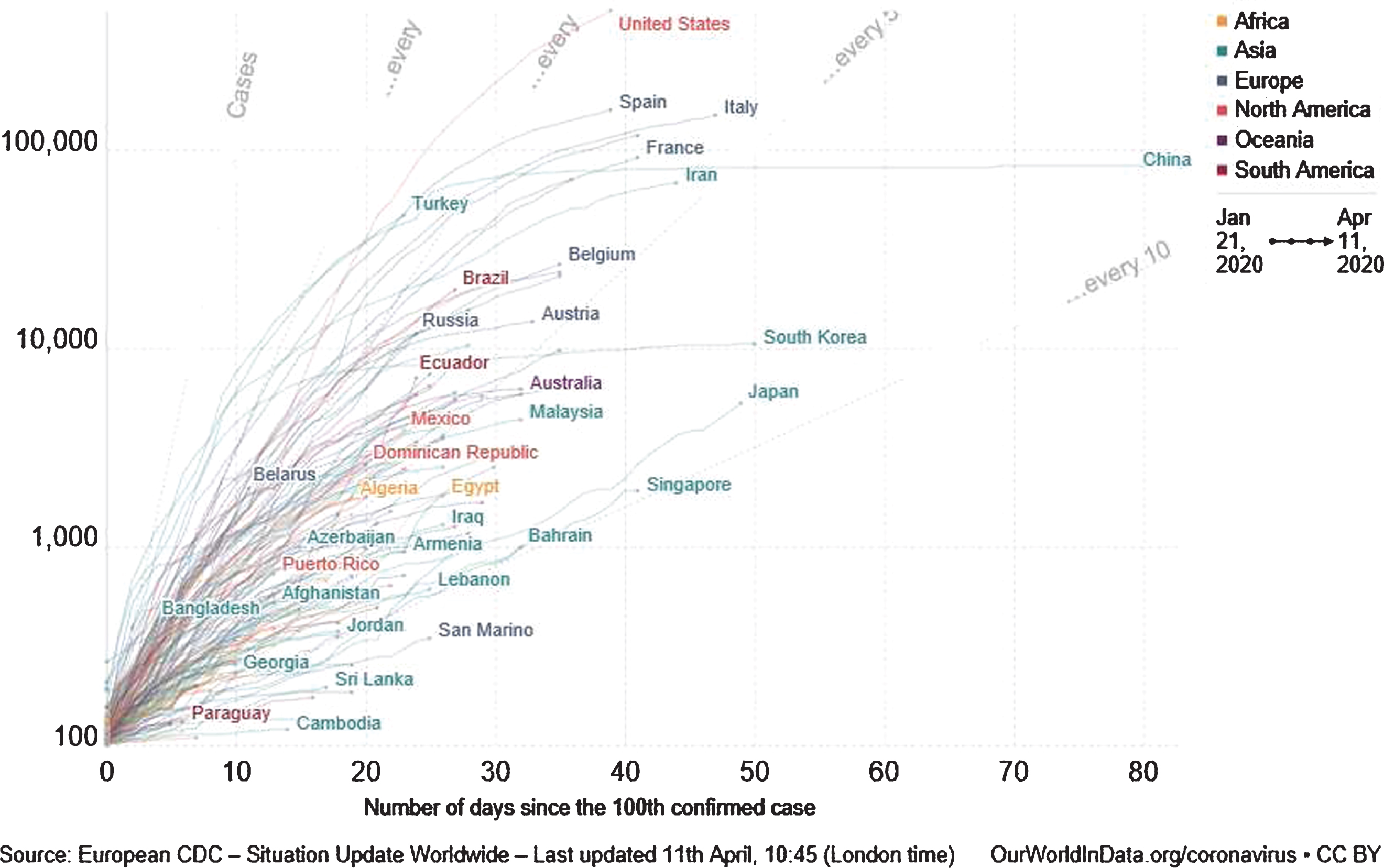
The COVID-19 has appeared as a deadly infection that has origins from China. The primary case was identified on December 31, 2019, in the city of Wuhan China, which is the capital of Hubei province. This fatal virus has taken the entire world into connections and multiple people have embraced death due to this insuperable virus. The name “coronavirus” comes from the Latin word “corona” which means a “crown, circle of light or nimbus”. This virus influences immediately to your lungs. It has comparable symptoms as influenza and pneumonia. In the beginning, various of those infected worked or shopped at a wholesale seafood market in Wuhan, China. After that it radiates universally through import, export, traveling, and social contacting of infected people. The Fig. 1 represents the world wide confirmed cases till 11th April 2020. Many researchers examined and established various techniques to deal with medical and decision-making obstacles. This manuscript proposes the most proficient technique for surviving from COVID-19, besides pharmaceutical medications. For this purpose, we investigated the MPNS, which was first discovered in 2020 by Hashmi et al. [16]. They preceded MPNS-topology and presented its applications in medical and clustering analysis. If we accumulate the data and conclude the decision without examining ambiguities, then given results will be boundless and obscure. For this purpose, a fuzzy set (FS) was established by Zadeh [44] in 1965 which is an imperative precise erection to epitomize an assembling of items whose boundary is ambiguous. After that, various hybrid models of FSs have been presented and investigated such as, intuitionistic fuzzy set (IFS) [5], single-valued neutrosophic set (SVNS) [31, 32], bipolar fuzzy set (BFS) [48–50], m-polar fuzzy set (MPFS) [9] and interval-valued fuzzy set (IVFS) [45]. The generality of the bipolar fuzzy set was originated by Chen [9] named as MPFS.
Fig. 1
World wide confirmed cases COVID-19.
The multi-criteria decision-making (MCDM) method is a sub-field of operations research that explicitly estimates multiple adverse measures in decision-making, business, medicine, engineering, artificial intelligence, and daily life problems. It is perceived as the intellectual process which fallouts the selection of a belief or a class of activity among various alternative possibilities according to diverse standards. Aggregation implies the invention of a numeral of things into a cluster or a bunch of objects that have come or been taken together. In the past few years, aggregation operators based on FSs and its various hybrid compositions have made very much attention and become attractive because they can quickly execute functional areas of diverse regions. Xu et al. [38–40] introduced weighted averaging operators, geometric operators and induced generalized operators based on IFNs. Ashraf et al. [2–4] studied spherical fuzzy sets and established its various aggregation operators with applications in decision-making problems. Jose and Kuriaskose [17] investigated aggregation operators with the corresponding score function for MCDM in the context of IFNs. Mahmood et al. [20] established generalized aggregation operators for CHFNs and use it into MCDM.
Riaz and Hashmi [25–27] established cubic m-polar fuzzy aggregation operators and presented multi-attribute group decision-making (MAGDM) to solve agribusiness problems. They introduced the new concept of linear Diophantine fuzzy sets (LDFSs). They introduced the novel structures of Pythagorean m-polar fuzzy soft rough sets (PMPFSRSs) and soft rough Pythagorean m-polar fuzzy sets (SRPMPFSs). They presented new algorithms based on LDFSs, PMPFSRSs, and SRPMPFSs to solve decision-making problems. Riaz et al. [28–30] introduced N-soft topology, soft rough topology, cubic bipolar fuzzy ordered weighted geometric aggregation operators with their applications in multi-criteria group decision-making (MCGDM) problems.
Ali [1] write a note on soft, rough soft and fuzzy soft sets. Qurashi and Shabir [24] presented generalized approximations of (∈ , ∈ ∨ q)-fuzzy ideals in quantales. Shabir and Ali [33] established some properties of soft ideals and generalized fuzzy ideals in semigroups. Xueling et al. [36] introduced decision-making methods based on various hybrid soft sets. Feng et al. [11–13] introduced properties of soft sets combined with fuzzy and rough sets and MADM models in the environment of generalized IF soft set and fuzzy soft set. Garg [14, 15] established trigonometric operation based q-ROF aggregation and neutrality operation based Pythagorean Fuzzy aggregation operators with their applications in decision-making problems. Peng et al. [21–23] introduced information measures on Pythagorean fuzzy sets and q-ROFSs and their applications. Boran et al. [8] use TOPSIS decision-making method for the supplier selection in the context of IFS. Varol and Aygun [34] established various results on fuzzy soft topological space. Aygünoglu et al. [7] introduced some results on fuzzy soft topology. Liu et al. [18] worked on hesitant IF linguistic operators and presented its MAGDM problem. Li et al. [19] established Einstein aggregation operators by using simplified neutrosphic numbers and presented its application in the decision-making problem. Wei et al. [35] established hesitant triangular fuzzy operators in MADGDM problems. A book on HFS was established by Xu [37] with the concept of its various aggregation operations and MCDM. Ye [41–43] introduced prioritized aggregation operators in the context of IVHFS and worked on its MAGDM. He also established MCDM methods for interval neutrosophic sets and simplified neutrosophic sets. Zhang et al. [46] introduced aggregation operators with MCDM by using interval-valued FNS (IVFNS). An extended TOPSIS method for decision-making was developed by Chi and Lui [10] on IVFNS Zhao [47] et al. worked on generalized aggregation operators in the context of IFS. Aiwu et al. [6] constructed generalized aggregation operator for INFNS.
The motivation of this hybrid work is provided step by step in the entire manuscript. We discuss the efficiency, docility, integrity, and perfection of our proposed aggregation techniques. MPNS and its generalized aggregation operators utilize to accumulate information data at a comprehensive scale and efficiently applicable in medical, engineering, artificial intelligence, agriculture, and other daily life problems. Doctors are providing precautions and directions to counter novel COVID-19. They also working on the strategies to get cured of this infection. We use our proposed models to diagnose this disease and to examine the comprehensive medical history of the victim from infected to cured. The suggested techniques help the physicians to choose the most desirable treatment and medication for fast convergence to the recovery of the patient.
The layout of this article is organized as follows. In Section 2, we study some fascinating theories of FSs, MPFSs, neutrosophic sets, and MPNSs. We examine some of its operations, score function, and improved score function. In Section 3, we use MPNS to establish novel generalized weighted and generalized Einstein weighted aggregation operators. In Section 4, we establish a novel technique based on the medical diagnosis of COVID-19 using presented aggregated operators by the constructed algorithms. This modeling diagnoses the disease and also works on data collection and evaluation history of the patient’s improvement report. In the sequence, we make a brief comparative analysis of proposed operators with some existing techniques. We discuss the influence and sensitivity of parameter ð to the recovery graphs. Eventually, some future directions and conclusions of this analysis are summarized in Section 5.
2Preliminaries
In this part, we examine some fundamental theories of fuzzy, neutrosophic, MPFSs and MPNSs. In the entire manuscript, we use
Definition 2.1. [44] A fuzzy set (FS)
Definition 2.2. [31] A neutrosophic set
Definition 2.3. [9] An m-polar fuzzy set (MPFS) is generalized model of bipolar fuzzy set (BFS) ([48–50]). The mapping
Definition 2.4. [16] An object
Table 1
MPNS
|
| MPNNs |
| ς1 |
|
| ς2 |
|
| . . . | . . . . . . . . . |
| . . . . . . . . . . . . | |
|
|
|
The notion
Definition 2.5. An empty MPNS can be scripted as
Definition 2.6. [16] We studies some operations for MPNNs
(i):
(ii):
(iii):
(iv):
(v):
Example 2.7. Consider two 4PNNs
Table 2
4PNNs
| 4PNNs | Numeric values of 4PNNs |
|
| (〈0.611, 0.111, 0.251〉, 〈0.821, 0.631, 0.111〉, 〈0.721, 0.381, 0.591〉, 〈0.211, 0.321, 0.411〉) |
|
| (〈0.321, 0.621, 0.511〉, 〈0.831, 0.111, 0.921〉, 〈0.521, 0.431, 0.391〉, 〈0.181, 0.931, 0.821〉) |
Table 3
Union and intersection of 4PNNs
| 4PNNs | Numeric values of 4PNNs |
|
| (〈0.611, 0.111, 0.251〉, 〈0.831, 0.111, 0.111〉, 〈0.721, 0.381, 0.391〉, 〈0.211, 0.321, 0.411〉) |
|
| (〈0.321, 0.621, 0.511〉, 〈0.821, 0.631, 0.921〉, 〈0.521, 0.431, 0.591〉, 〈0.181, 0.931, 0.821〉) |
Definition 2.8. Sometimes, we use MPNNs to solve multi-attribute, multi-criteria and group decision-making problems. During the formation of diverse algorithms, we get the optimized resolutions and we need to order the concerned MPNNs to perceive the most beneficial and relevant judgment. For this purpose, we have to define some score functions corresponding to MPNN
Definition 2.9. [16] Let
(a): If
(b): If
(1): If
(2): If
(i): If
(ii): If
(iii): If
Example 2.10. Consider two 2PNNs
By Definition 2.8
Remark.
•For null MPNN
•For absolute MPNN
Definition 2.11. [16] Let
1.
2.
3.
4.
Remark.
3Generalized aggregation operators
In this section, we establish m-polar neutrosophic generalized weighted aggregation (MPNGWA) and m-polar neutrosophic generalized Einstein weighted aggregation (MPNGEWA) operators. We present some special cases of established operators for different values of parameter ð.
3.1m-polar neutrosophic generalized weighted aggregation (MPNGWA) operator
Definition 3.1. Let ℧ be an assembling of MPNNs
Now we establish some new operators from MPNGWA operator for different values of parameter ð.
1. When ð→0 then MPNGWA operator reduces to m-polar neutrosophic weighted geometric aggregation (MPNWGA) operator defined as:
2. When ð=1 then MPNGWA operator reduces to m-polar neutrosophic weighted arithmetic aggregation (MPNWAA) operator defined as:
Let
Table 5
3PNNs
| 3PNNs | Numeric values of 3PNNs |
|
| (〈0.81, 0.24, 0.31〉, 〈0.56, 0.43, 0.28〉, 〈0.61, 0.71, 0.38〉) |
|
| (〈0.91, 0.32, 0.41〉, 〈0.73, 0.15, 0.23〉, 〈0.34, 0.25, 0.61〉) |
|
| (〈0.36, 0.21, 0.41〉, 〈0.91, 0.85, 0.34〉, 〈0.73, 0.35, 0.25〉) |
Example 3.2. Consider three 3PNNs
Table 4
2PNNs
| 2PNNs | Numeric values of 2PNNs |
|
| (〈0.5, 0.3, 0.4〉, 〈0.5, 0.1, 0.8〉) |
|
| (〈0.2, 0.3, 0.1〉, 〈0.2, 0.1, 0.5〉) |
3.2m-polar neutrosophic generalized einstein weighted aggregation (MPNGEWA) operator
There exists some limitations in the defined operations of MPNNs. In general sense, the sum of any number with the maximal number is equal to maximal value and the multiplication of minimal number to any number is equal to the any one. But our defined operations contradict these rules in general. For example,
1.
2.
3.
4.
Definition 3.3. Let ℧ be an assembling of MPNNs
3.3Properties and special cases of MPNGEWA operator
The MPNGEWA operator has the following properties.
1. Idempotency: Let
2. Commutativity: Let
3. Boundedness: Let
4. Monotonicity: Let
Now we discuss some cases of MPNGEWA operator based on the parameter ð.
1. When ð=1 then MPNGEWA operator reduces to the m-polar neutrosophic Einstein weighted average (MPNEWA) operator. Therefore,
So, MPNEWA operator for
2. When ð = -1 then MPNGEWA operator reduces to the m-polar neutrosophic Einstein weighted harmonic average (MPNEWHA) operator. Therefore,
So, MPNEWA operator3. When ð→0 then MPNGEWA operator reduces to the m-polar neutrosophic Einstein weighted geometric average (MPNEWGA) operator for
Example 3.4. Consider that we have three 3PNNs given as Table 6. For the weight vector ζ = (0.3, 0.4, 0.3) T and parameter ð=1, we calculate the aggregated value by using MPNGEWA operator for
Table 6
3PNNs
| 3PNNs | Numeric values of 3PNNs |
|
| (〈0.81, 0.24, 0.31〉, 〈0.56, 0.43, 0.28〉, 〈0.61, 0.71, 0.38〉) |
|
| (〈0.91, 0.32, 0.41〉, 〈0.73, 0.15, 0.23〉, 〈0.34, 0.25, 0.61〉) |
|
| (〈0.36, 0.21, 0.41〉, 〈0.91, 0.85, 0.34〉, 〈0.73, 0.35, 0.25〉) |
Similarly,
Thus by using equation (Z) of MPNGEWA operator for
4Multi-criteria decision-making for diagnosis of COVID-19
In this section, we present an innovative technique to diagnose the COVID-19 of a patient by using Mathematical modeling through proposed aggregation operators. With the help of parameter ð, we can examine the comprehensive medical history of the victim from infected to cured. The suggested techniques help the physicians to choose the most desirable treatment and medication for fast convergence to the recovery of the patient.
4.1Proposed technique
In this part of our manuscript, we establish the techniques of MPNGWA and MPNGEWA operators to detect the disease of the patient in the environment of MPN-data.
Input:
Step 1: The following
Step 2: In business term we mostly consider two main attribute terms including, benefit and cost. In MCDM the greatest value of benefit attribute and lower value of cost attribute leads us to success. The value of loss attribute case can be converted into value of benefit attribute by normalizing the input data
Calculations:
Step 3(a): Compute the aggregated values of alternatives
Step 3(b): Compute the aggregated values of alternatives
Output:
Step 4: Using
Step 5: We rank these alternative on the basis of score values according to the Definition 2.9.
Step 6: Choose the alternative with the maximum score calculated through the purposed method.
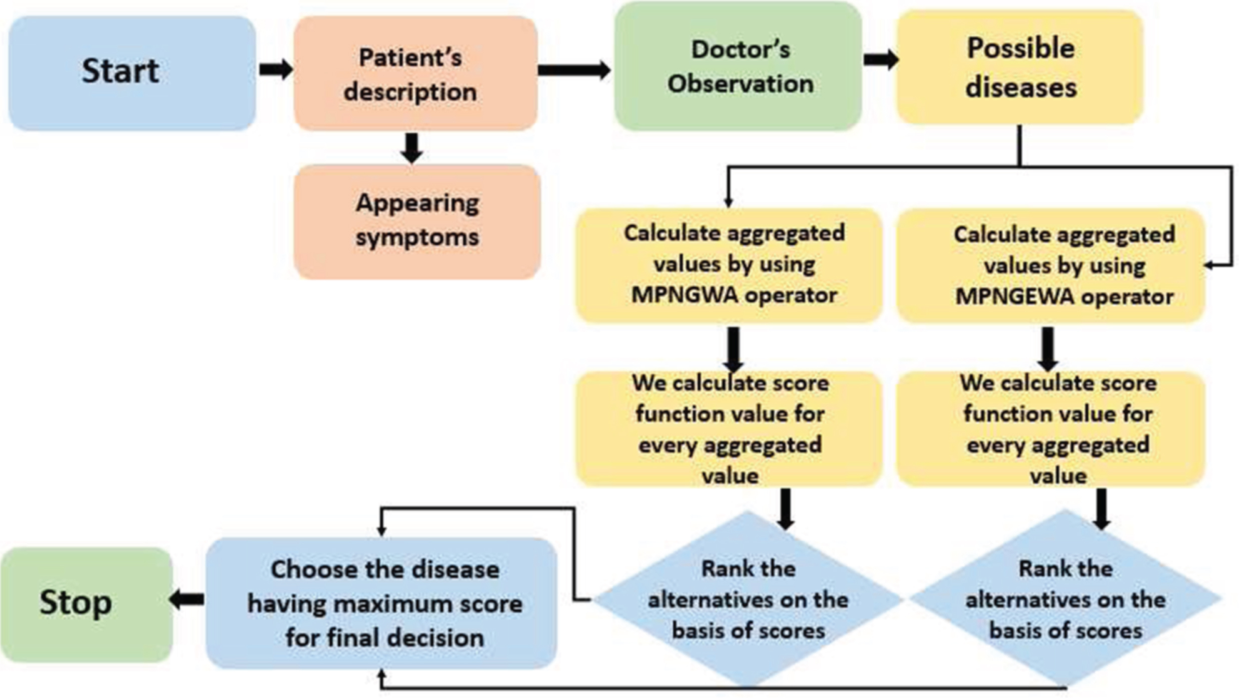
The flow chart diagram of proposed algorithm can be seen in Fig. 2.
Fig. 2
Flow chart diagram of proposed algorithms to diagnose COVID-19.
Algorithm 1 Algorithm to diagnose COVID-19 using MPNGWA operator
1: procedure ApplyMPNGWA
2: Input: collection of input MPN-data in decision matrix
3: Output: collection of input MPN-data
4: for ℘=1 to
5: for to
6: if
7:
8: else
9:
10: end if
11: end for
12: end for
13: for ℘=1 to
14: for ℘′=1 to
15: for ð=1 to 10000
16:
17: end for
18: end for
19: end for
20: for ℘′=1 to
21: Compute
22: end for
23: Rank the alternatives
24: end procedure
4.2Case study
For a short time interval, the contagious disease which spread instantly among the inhabitants is called epidemic disease. There are diverse epidemic models for infectious diseases, but we argue here about the SIR model for the given decision-making problem. The SIR model is a mathematical model of infectious diseases, where we have three compartments given as;
S= “Susceptible”,
I= “Infected or infectious”,
R= “Recover or removed”.
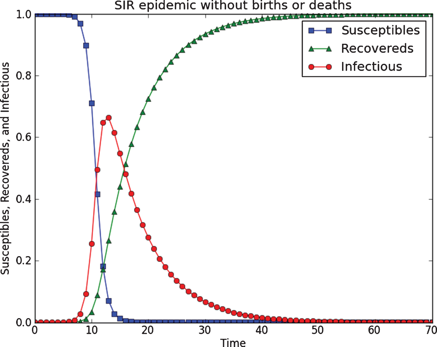
For the development of such types of models, we develop some hypotheses according to the model and circumstances. We are working for the diagnosis, so we consider a very simple and fundamental model with no death and birth rates given in Fig. 3. The variation in the population of every compartment with the rates b and r can be seen graphically as Fig. 4. We can add death and birth rates to the SIR model for further modification. From the last year, the epidemic disease named as coronavirus (COVID-19) has been spreading very fast among the humans. This effects directly to your lungs. It has similar symptoms as influenza and pneumonia. The X-ray images of infected persons are given in Figs. 5 and 6. “In Fig. 5 represents the chest CT images of a 29-year-old man with fever for 6 days. RT-PCR assay for the SARS-CoV-2 using a swab sample was performed on Feb. 5, 2020, with a positive result. (A column) Normal chest CT with axial and coronal planes was obtained at the onset. (B column) Chest CT with axial and coronal planes shows minimal ground-glass opacities in the bilateral lower lung lobes (yellow arrows). (C column) Chest CT with axial and coronal planes shows increased ground-glass opacities (yellow arrowheads). (D column) Chest CT with axial and coronal planes shows the progression of pneumonia with mixed ground-glass opacities and linear opacities in the subpleural area. (E column) Chest CT with axial and coronal planes shows the absorption of both ground-glass opacities and organizing pneumonia”.
Algorithm 2 Algorithm to diagnose COVID-19 using MPNGEWA operator
1: procedure ApplyMPNGEWA
2: Input: collection of input MPN-data in decision matrix
3: Output: collection of input MPN-data
4: for ℘=1 to
5: for ℘′=1 to
6: if
7:
8: else
9:
10: end if
11: end for
12: end for
13: for ℘=1 to
14: for ℘′=1 to
15: for ð=1 to 10000
16:
17: end for
18: end for
19: end for
20: for ℘′=1 to
21: Compute
22: end for
23: rank the alternatives
24: end procedure
Fig. 3
SIR model for epidemic diseases.
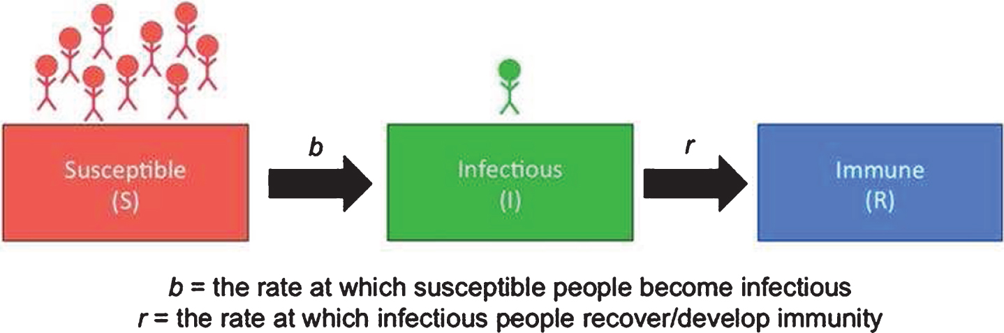
Fig. 4
Graphical representation of SIR model.
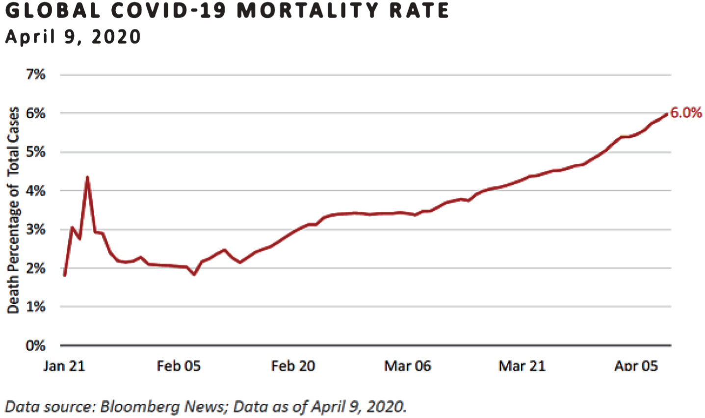
This virus banquets predominantly through discharge from the nose or droplets of saliva when a disease-ridden person sneezes or coughs. Patients suffering from COVID-19 usually experience mild to the severe respiratory issue. Other key warning signs may consist of high-grade fever (usually more than 100 F) or chills, cough, vomiting, and shortness of breath. These symptoms may appear from 2 days to a couple of weeks after exposure. There may be some other symptoms like tiredness, runny nose, aches, and sore throat. The deadly virus has not only taken the lives of a number of people but also has shattered the economy of most established and developed countries. The Fig. 7 represents the global increase in reported COVID-19 cases. According to statistics, the death rate of individuals of age 80+ is 21.9% due to COVID-19 (confirmed cases) as compared to a overall death rate of 14.8% in all cases among the same age group. Moreover, the death rate among males is 4.7% whereas in females is 2.8% out of confirmed cases of COVID-19. The graph of worldwide death rate (till 11th April 2020) due to COVID-19 is portrayed in Fig. 8.
Fig. 5
Chest CT images of infected person with coronavirus.
Source: https://www.itnonline.com/sites/itnonline/files/styles/content-large.
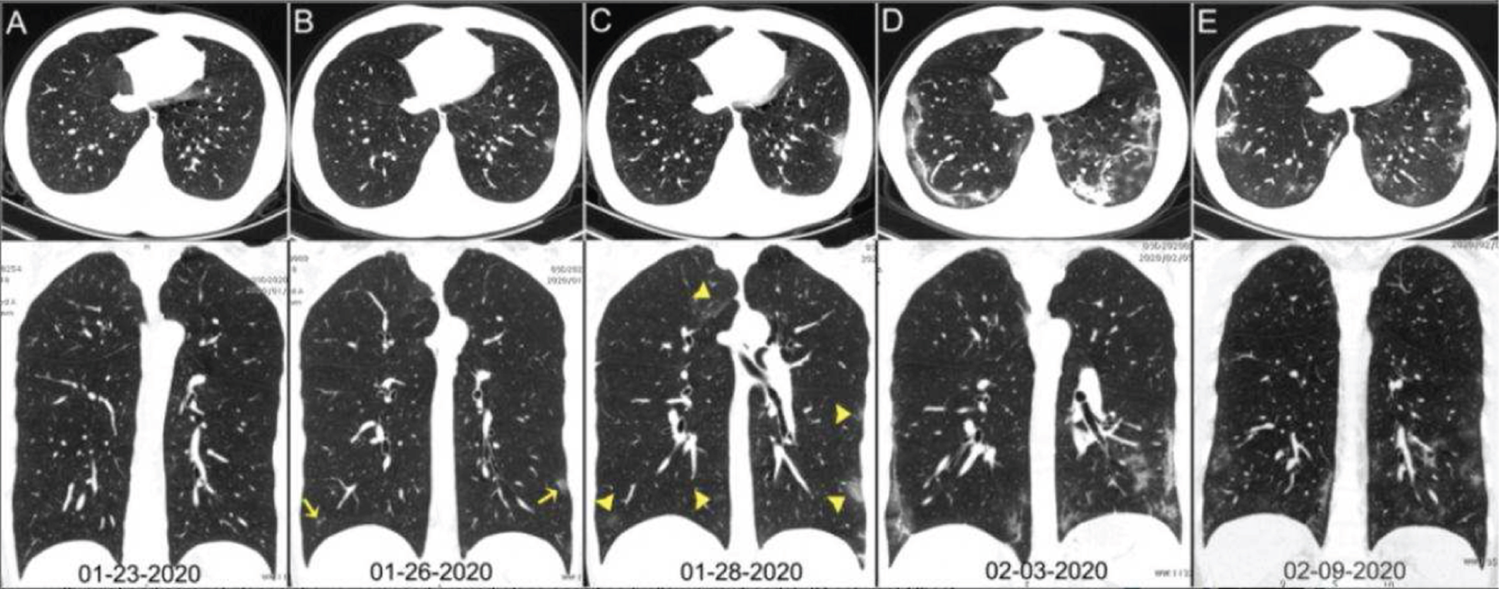
Fig. 6
Four COVID-19 lung CT scans (top) with corresponding colored maps showing coronavirus abnormalities (bottom). Source:hospitals-deploy-ai-tools-detect-covid19-chest-scans.
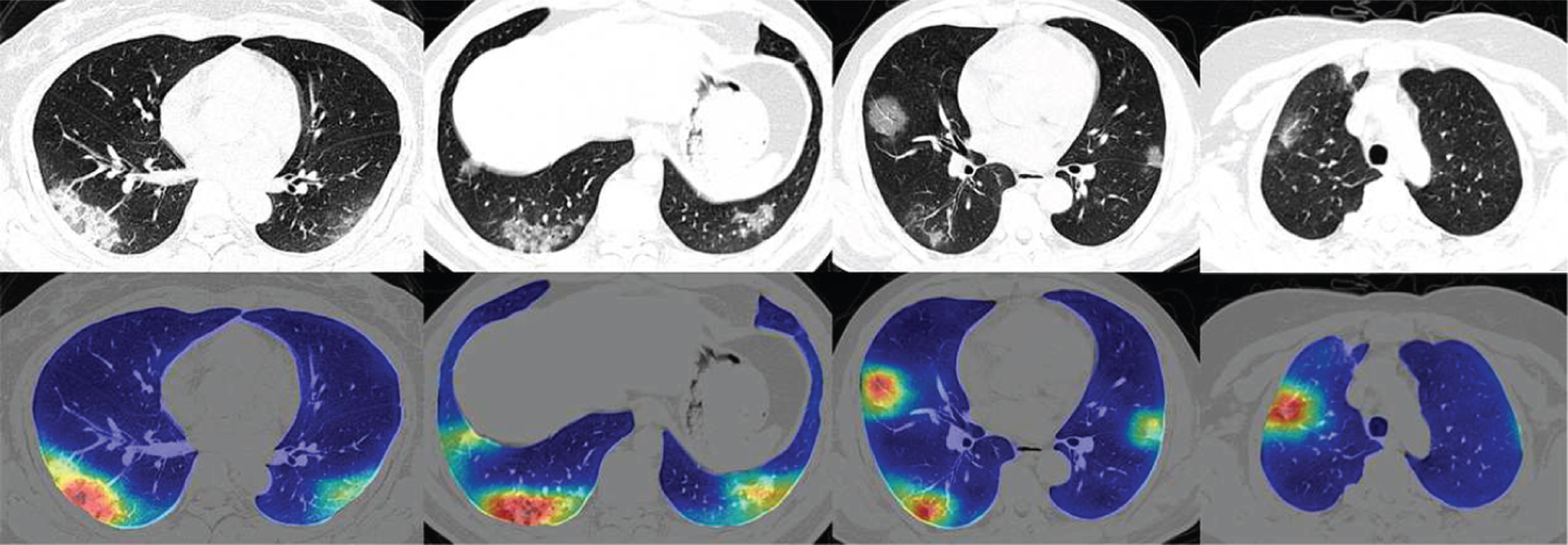
Fig. 7
Global increase in reported COVID-19 cases.
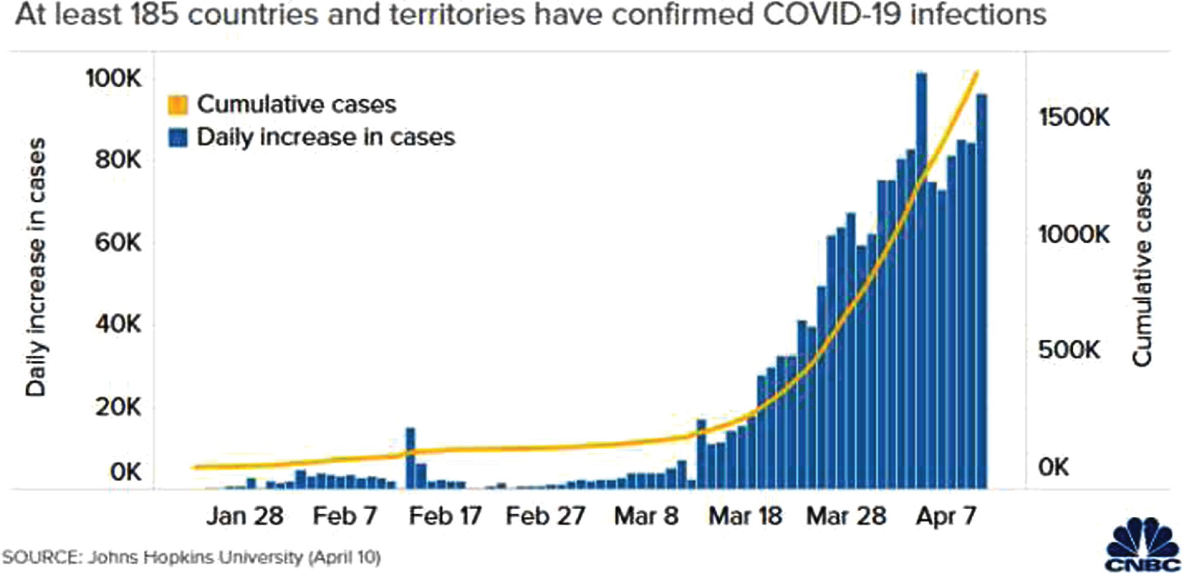
Fig. 8
Worldwide death rate due to COVID-19.
4.3Numerical example
A man visits a doctor and told him about his health problems which he was facing for the last three days. He stated that he was suffering from a cough and high fever. He mentions that he has a runny nose with a sore throat. He also feels muscle pain with a headache. Granting to the doctor all the symptoms lead to three diseases coronavirus, influenza, and pneumonia. It is challenging for a physician to diagnose the exact disease of this patient without any medical test because on that point is an overlapping between the symptoms of above-named diseases. We present two novel algorithms with new models of MPNGWA and MPNGEWA operators to diagnose the disease of the patient and we also discuss the recovery of the patient.
Mathematical modeling: For the given case study we have a set of alternatives consists of three diseases
Granting to the patient’s description, the doctor can place a weighted vector ζ = (0.2, 0.1, 0.1, 0.1, 0.2, 0.3) T according to the diseases and symptoms. This vector is selected by using Table refdata set. We choose
Table 7
3PN-data
| Order | 3PNNs | Numeric values of 3PNNs |
| 1 |
|
|
| 2 |
|
|
| 3 |
|
|
| 4 |
|
|
| 5 |
|
|
| 6 |
|
|
| 1 |
|
|
| 2 |
|
|
| 3 |
|
|
| 4 |
|
|
| 5 |
|
|
| 6 |
|
|
| 1 |
|
|
| 2 |
|
|
| 3 |
|
|
| 4 |
|
|
| 5 |
|
|
| 6 |
|
|
Table 8
Data set for appearing symptoms
| Appearing symptom | Mild or Low | Moderate | Severe |
| Cough | 0 ≤ ς < 0.1 | 0.1 ≤ ς < 0.2 | 0.2 ≤ ς ≤ 1 |
| Headache | 0 ≤ ς < 0.1 | 0.1 ≤ ς < 0.2 | 0.2 ≤ ς ≤ 1 |
| Runny nose | 0 ≤ ς < 0.1 | 0.1 ≤ ς < 0.2 | 0.2 ≤ ς ≤ 1 |
| Muscle pain | 0 ≤ ς < 0.1 | 0.1 ≤ ς < 0.2 | 0.2 ≤ ς ≤ 1 |
| Sore Throat | 0 ≤ ς < 0.1 | 0.1 ≤ ς < 0.2 | 0.2 ≤ ς ≤ 1 |
| High fever | 0 ≤ ς < 0.1 | 0.1 ≤ ς < 0.2 | 0.2 ≤ ς ≤ 1 |
Calculations by using MPNGWA operator:
Then by using 3PNGWA operator from equation (A) over the input data for ð=1 (equivalent to 3PNWAA operator from equation (C)) we get,
We use improved score function £3 to calculate score values because it gives better and accurate results as compared to £1 and £2. Hence the score values of above aggregated 3PNNs can be obtained by using Definition 2.8 given as,
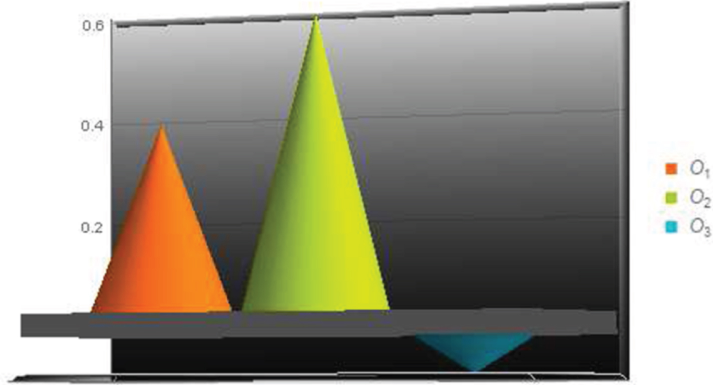
Which shows that patient should get serious about his health, because he is suffering from COVID-19. This ranking can be seen graphically as Fig. 9.
Fig. 9
Ranking of 3PNNs
Calculations by using MPNGEWA operator:
Then by using 3PNGEWA operator from equation (Z) over the input data for ð=1 (equivalent to 3PNEWA operator from equation (Z*)) we get,
We use improved score function £3 to calculate score values because it gives better an accurate results as compared to £1 and £2. Hence the score values of above aggregated 3PNNs can be obtained by using Definition 2.8 given as,
The Influence and Sensitivity of Parameter ð:
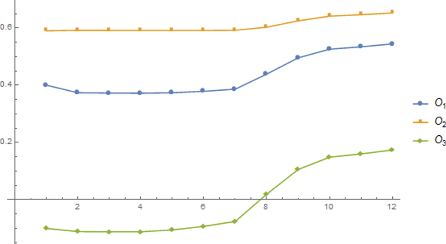
We calculate the aggregated 3PNNs for different values of parameter ð from the input 3PN-data under 3PNGWA and 3PNEGWA operators. The behavior of both operators can be observed from Tables 9 and 10 under the effect of parameter ð. The parameter ð has no consequence on the ranking results of MPNGWA and MPNEGWA operators. This signifies that the obtained ranking results from both operators are not sensitive to the parameter ð. For a very large value of parameter ð every aggregated MPNN approaches to null MPNN. This represents that there will be no variations in the process and results remains constant. The answers show that both operators are more elastic and desirable for the MCDM problems. The ranking results of MPNNs for both operators can be graphically represented as Figs. 10 and 11.
Table 9
Ranking under the MPNGWA operator for different values of ð
| ð | Type of operator |
| Ranking order | Result |
| →0 | MPNWGA | 0.3164, 0.5731, - 0.1527 |
|
|
| 0.1 | MPNGWA | 0.3781, 0.5911, - 0.1097 |
|
|
| 0.3 | MPNGWA | 0.3804, 0.5914, - 0.1063 |
|
|
| 0.5 | MPNGWA | 0.3826, 0.5918, - 0.1028 |
|
|
| 1 | MPNWAA | 0.3883, 0.5928, - 0.0934 |
|
|
| 1.5 | MPNGWA | 0.3940, 0.5937, - 0.0833 |
|
|
| 2 | MPNGWA | 0.3996, 0.5948, - 0.0727 |
|
|
| 5 | MPNGWA | 0.4304, 0.6012, - 0.0097 |
|
|
| 10 | MPNGWA | 0.4697, 0.6126, 0.0658 |
|
|
| 15 | MPNGWA | 0.4974, 0.6235, 0.1114 |
|
|
| 17 | MPNGWA | 0.5061, 0.6275, 0.1246 |
|
|
| 20 | MPNGWA | 0.5172, 0.6330, 0.1407 |
|
|
Table 10
Ranking under the MPNGEWA operator for different values of ð
| ð | Type of operator |
| Ranking order | Result |
| →0 | MPNEWGA | 0.4000, 0.5900, - 0.1000 |
|
|
| 0.1 | MPNGEWA | 0.3737, 0.5918, - 0.1109 |
|
|
| 0.3 | MPNGEWA | 0.3726, 0.5915, - 0.1118 |
|
|
| 0.5 | MPNGEWA | 0.3721, 0.5914, - 0.1116 |
|
|
| 1 | MPNEWAA | 0.3736, 0.5912, - 0.1053 |
|
|
| 1.5 | MPNGEWA | 0.3787, 0.5914, - 0.0925 |
|
|
| 2 | MPNGEWA | 0.3861, 0.5920, - 0.0758 |
|
|
| 5 | MPNGEWA | 0.4387, 0.6025, - 0.0194 |
|
|
| 10 | MPNGEWA | 0.4957, 0.6248, 0.1058 |
|
|
| 15 | MPNGEWA | 0.5258, 0.6413, 0.1488 |
|
|
| 17 | MPNGEWA | 0.5342, 0.6463, 0.1603 |
|
|
| 20 | MPNGEWA | 0.5444, 0.6526, 0.1738 |
|
|
Fig. 10
Ranking of MPFNNs for MPNGWA operator.
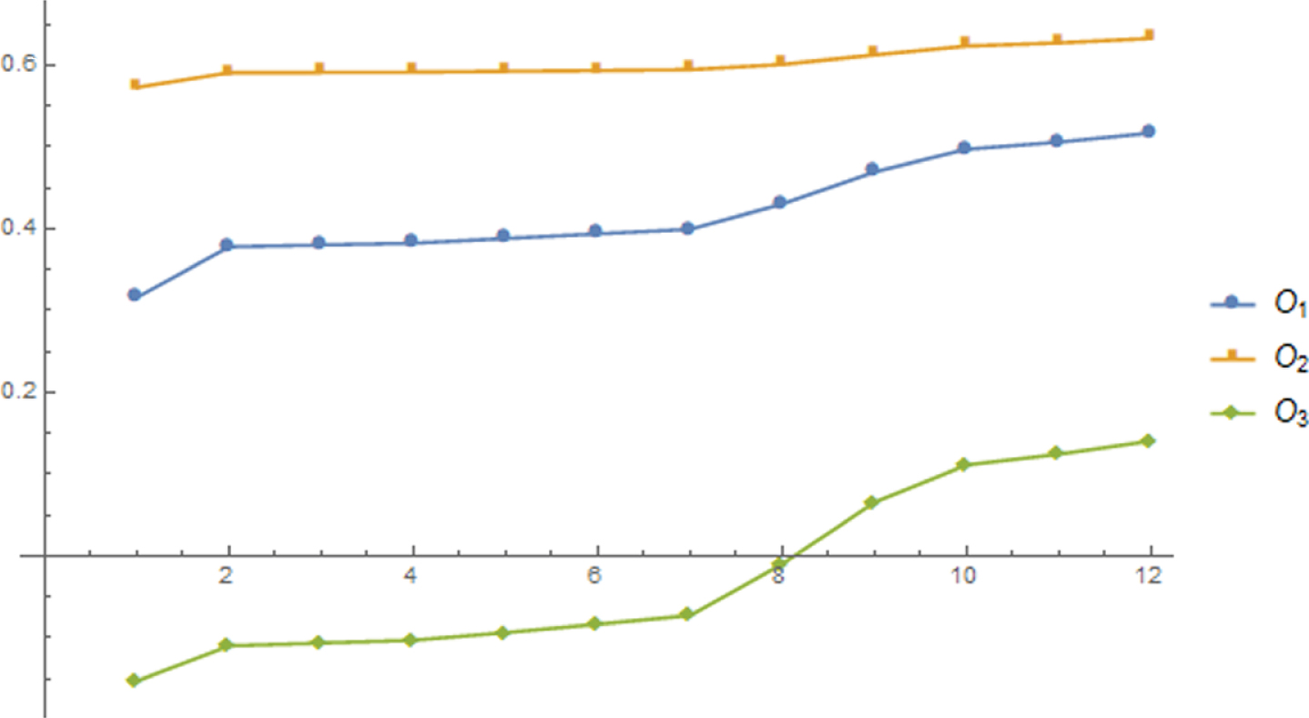
Fig. 11
Ranking of MPFNNs for MPNGEWA operator.
4.4Convergence in recovery of the patient
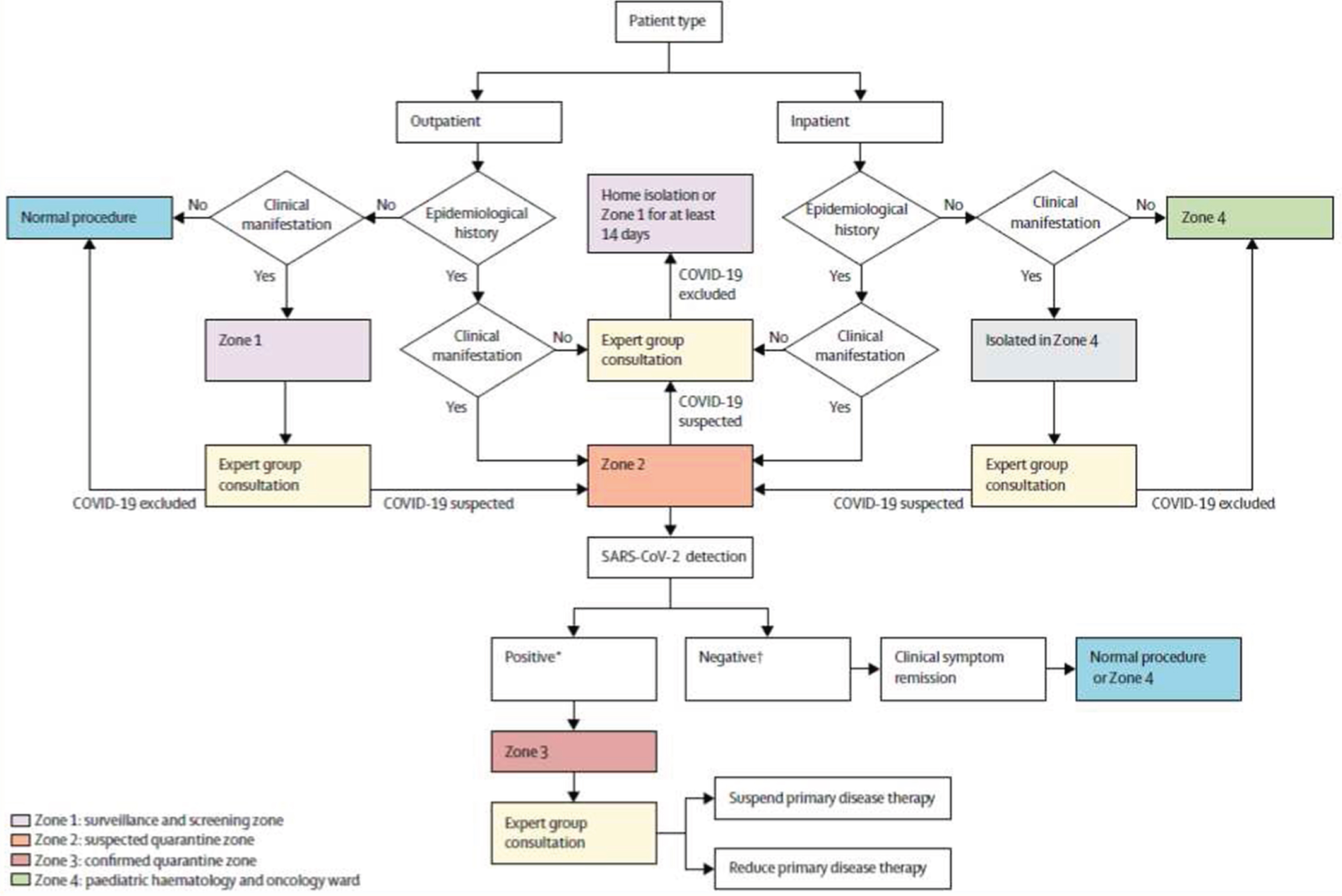
All the previous process shows that how to diagnose the disease of a patient with mathematical modeling under the environment of MPN-data. In this subsection, we use above modeling to determine that how much time and factors are postulated for a patient to recuperate from that disease. From above discussion, we know that decision goes for COVID-19. Till to date, there are no explicit serums or treatments for COVID-19. Though, there are several ongoing clinical trials assessing latent treatments. The “strategic plan for management of COVID-19 in paediatric haematology and oncology departments”is given in Fig. 12.
Fig. 12
Strategic plan for management of COVID-19 in paediatric haematology and oncology departments.
For initial and smaller values of parameter ð in proposed operators, we see the performance of aggregated MPNN and its score value for both operators. It is clear from the calculations (see Tables 11 and 12) and graphical representation (see Graphs 13 and 14) that initially its score valued increases means that disease is uncured and the patient is infected and its infection is increasing day by day. After diagnosis, the Doctor starts his treatment, according to the necessary medication and some preventions. The patient used those suggested medicines and stick with his complete diet plan with necessary precautions. Then by increasing the time period, his infection reduces and score values decrease for the larger values of the parameter. We relate the parameter ð with the time and treatment, so as to ð increases all the aggregated values go to null MPNNs for both operators. This proves that the patient is recovering from COVID-19. After just about a specific time and treatment score value goes to the minimum which is -1 and after that, no changes occur in score value with the changing of the parameter. This stands for that patient is entirely cured and it moves towards the recovering population from the infected population. The graphical views clearly express all the history of patient disease from start to end (see Figs. 13 and 14). Starting values show that he is infected and diagnosed with COVID-19. After diagnosis and treatment with the passage of time he gets cured of COVID-19 and last values show that he runs to the box of recovered population and he is nowadays out of peril. This mathematical modeling helps us to examine the perfect story of a patient from infected to regain. This mannequin can be offered for various diseases and for a great number of patients. Our proposed model is a more abstracted form of fuzzy set and utilizes to diagnose disease, development of patient’s history and gather data at a very big plate.
Table 11
Results depending on ð for Recovery of patient via MPNGWA operator
| ð | Score values | ð | Score values | ð | Score values | ð | Score values | ð | Score values |
| →0 | 0.5731 | 20 | 0.6330 | 136 | 0.6897 | 260 | 0.4755 | 1000 | -0.5105 |
| 0.1 | 0.5911 | 25 | 0.6411 | 137 | 0.6900 | 270 | 0.2760 | 1100 | -0.5104 |
| 0.3 | 0.5914 | 30 | 0.6479 | 138 | 0.6250 | 275 | 0.2763 | 1150 | -0.5104 |
| 0.5 | 0.5918 | 40 | 0.6583 | 139 | 0.6254 | 280 | 0.11276311 | 1190 | -0.5102 |
| 1 | 0.5928 | 50 | 0.6658 | 140 | 0.6250 | 285 | -0.0159 | 1192 | -0.5102 |
| 2 | 0.5748 | 70 | 0.6757 | 150 | 0.5577 | 300 | -0.0158 | 1193 | - 1 |
| 5 | 0.6012 | 100 | 0.6841 | 160 | 0.5582 | 400 | -0.0398 | 1200 | -1 |
| 10 | 0.6126 | 120 | 0.6876 | 180 | 0.5587 | 500 | -0.5109 | 1500 | -1 |
| 15 | 0.6235 | 130 | 0.6891 | 200 | 0.4849 | 700 | -0.5107 | 5000 | -1 |
| 17 | 0.6275 | 135 | 0.6892 | 250 | 0.4852 | 900 | -0.5105 | 10000 | -1 |
Table 12
Results depending on ð for Recovery of patient via MPNEGWA operator
| ð | Score values | ð | Score values | ð | Score values | ð | Score values | ð | Score values |
| →0 | 0.5900 | 20 | 0.6526 | 136 | 0.4851 | 260 | -0.5109 | 615 | -0.5104 |
| 0.1 | 0.5918 | 25 | 0.6608 | 137 | 0.4853 | 270 | -0.5109 | 616 | -0.5102 |
| 0.3 | 0.5915 | 30 | 0.6669 | 138 | 0.4851 | 275 | -0.5108 | 617 | - 1 |
| 0.5 | 0.5914 | 40 | 0.6754 | 139 | 0.4852 | 280 | -0.5108 | 618 | -1 |
| 1 | 0.5912 | 50 | 0.6810 | 140 | 0.4753 | 285 | -0.5108 | 619 | -1 |
| 2 | 0.5920 | 70 | 0.6879 | 150 | 0.2760 | 300 | -0.5108 | 620 | -1 |
| 5 | 0.6025 | 100 | 0.5590 | 160 | -0.0158 | 400 | -0.5106 | 700 | -1 |
| 10 | 0.6248 | 120 | 0.4850 | 180 | -0.0402 | 500 | -0.5105 | 1000 | -1 |
| 15 | 0.6413 | 130 | 0.4851 | 200 | -0.0400 | 600 | -0.5102 | 5000 | -1 |
| 17 | 0.6463 | 135 | 0.4852 | 250 | -0.5109 | 610 | -0.5104 | 10000 | -1 |
Fig. 13
Recovery graph of patient from COVID-19 via MPNGWA operator.
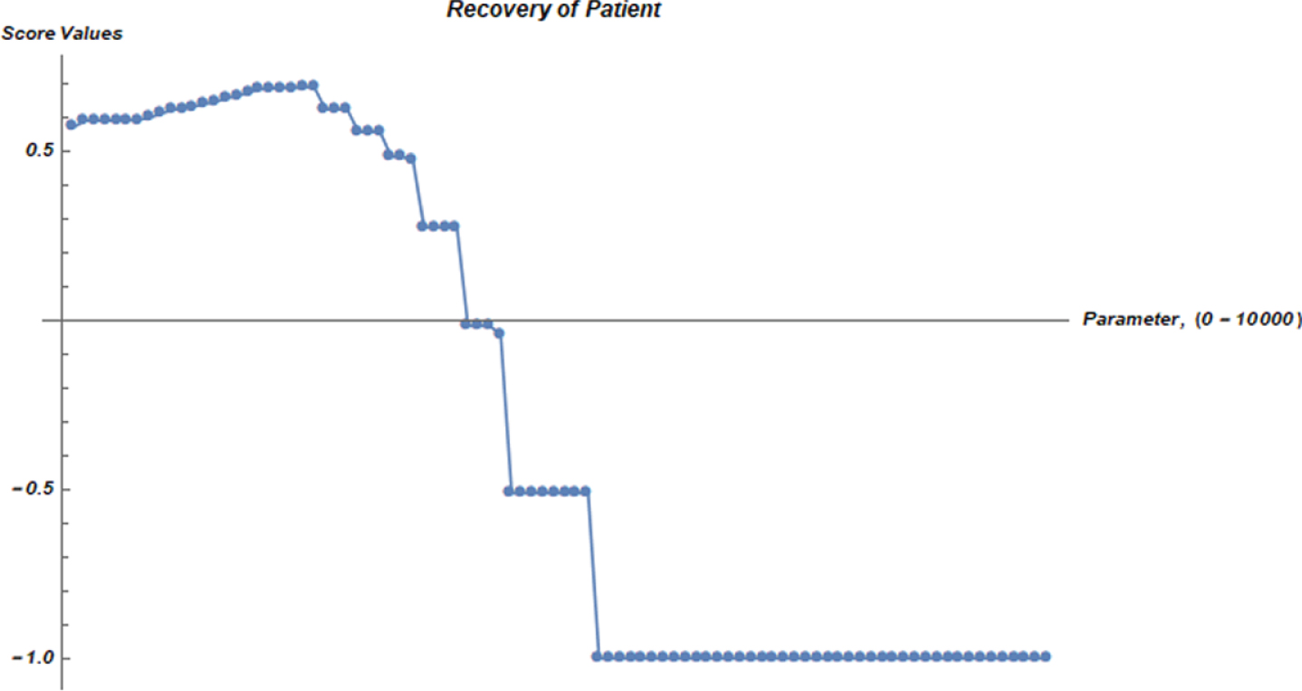
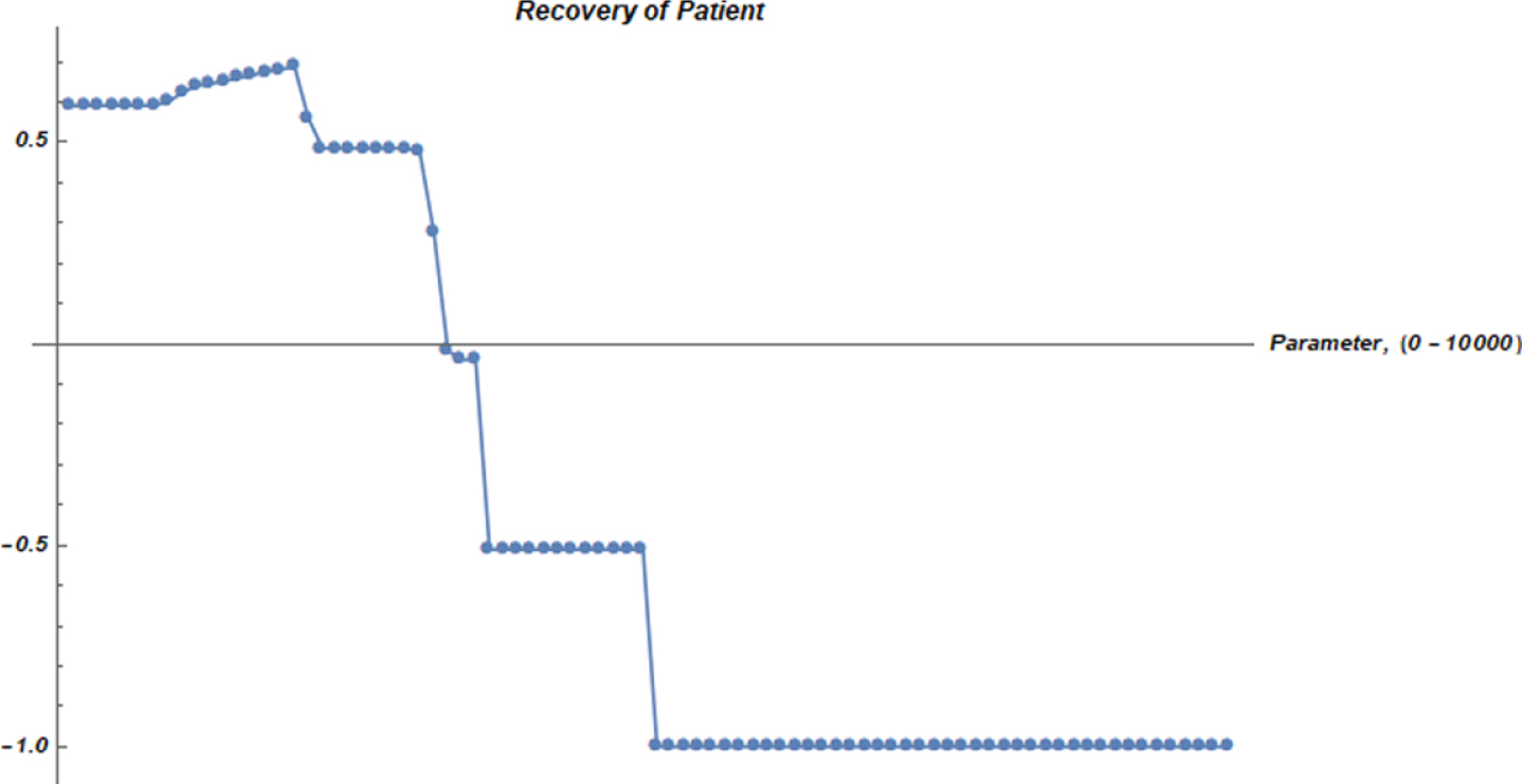
Fig. 14
Recovery graph of patient from COVID-19 via MPNEGWA operator.
4.5Comparison of MPNGWA and MPNGEWA operators
Both operators can give the appropriate and fast optimal solution as compared to the existing techniques. The convergence to the recovery of the patient can be observed by increasing the values of parameter ð. We relate the parameter ð with the time and treatment, so as to ð increases all the aggregated values go to null MPNNs for both operators. If we compare the results of both operators under the effect of different values of parameter ð from Tables 11 and 12, then we observe that both converge to value -1. The MPNGEWA operator is most suitable and gives faster convergence to the recovery of the patient as compared to the MPNGWA operator. In Table 11 we can see that MPNGWA operator converge the recovery value -1 at ð=1193. In Table 12 we can see that MPNGEWA operator converge the recovery value -1 at ð=617. This analysis shows that if we treat the patients (medication, visits, diet chart, etc) by using MPNGEWA operator then we can get the fast recovery as compared to other operators.
Comparison Analysis and Discussion:
In our proposed research, we defined generalized aggregated and generalized Einstein aggregated operators by using the advanced concept of MPNNs. The impressive point of this model is that we can use it for mathematical modeling at a large scale or
From Table 13, we can ensure that results obtained from different aggregation operators are similar to the proposed method. These results affirm that our proposed algorithm is authentic and correct. The final optimal decision is the same, but we get a slight difference between the overall ranking of the alternatives. This difference appears due to the different formulation and different algorithms for different aggregation operators. But the question turns out here that if we bring these resolutions from other operators, then why we need to specify a novel algorithm based on this novel structure? There are many arguments that show that the proposed operator is modified and generalized form others. Foremost of all we understand that due to the behavior of parameter ð we can as well examine the recovery of the patient and its complete graph history from beginning to end. But other operators such as IVIFWA [17] and IFWA, IFWG [38, 39] only diagnose the disease, but not covers the convergence of recovery of patients. Secondly, when we are dealing with [6, 17, 20, 38, 39, 47] operators then we face difficulties to collect the input data for all three weeks of the patient and observe no flexibility to deal with the various numbers of criteria with truth, falsity and indeterminacy degrees and all these ingredients make the calculations very difficult. Only when we are handling the data with MPNNs, then due to
Table 13
Comparison of different methods
| Methods | Operators | Ranking of alternatives |
| Aiwu [6] | IVNSGWA |
|
| Jose [17] | IVIFWA |
|
| Mahmood [20] | GCHFWA |
|
| Xu [38, 39] | IFWA,IFWG |
|
| Zaho [47] | GIFWA,GIVIFWA |
|
| Proposed method | MPNGWA |
|
| Proposed method ð=1 | MPNWAA |
|
| Proposed method ð→0 | MPNWGA |
|
| Proposed method | MPNGEWA |
|
| Proposed method ð=1 | MPNEWA |
|
| Proposed method ð→0 | MPNEWGA |
|
5Conclusion
In this manuscript, we have investigated MPNS and its various operations with scores and improved score functions. The generalized weighted aggregated and generalized Einstein weighted aggregated operators have been found by using the MPN operations. In the late years, many aggregation operators corresponding to numerous hybrid fuzzy sets have been instituted to deal with the MCDM problems. We have developed some hybrid generalized weighted aggregation operators based on MPNNs and use them into MCDM for medical diagnosis of COVID-19. We have calculated the aggregated results for different values of parameter ð=1 - 10, 000 and found the recovery results for the patients from COVID-19. Comparative analysis showed that these modified operators can easily solve real-life obstacles and decision-making problems. We can use them to collect information on a large scale for
In the future, this work can be gone easily for other approaches and different types of manipulators to solve problems of real-world including business, trade, medical, environmental sciences, social sciences, transportation analysis, pattern recognition, economics, human resource management, artificial intelligence, robotics, and many other areas. We will extend this work for MCDM optimization techniques such as TOPSIS, VIKOR, AHP and, PROMETHEE family. Researchers will get beneficial results by exploring and investigating these concepts in the field of MCDM by using numerous aggregation operators.
References
[1] | Ali M.I. , A note on soft sets, rough soft sets and fuzzy soft sets, Applied Soft Computing 11: ((2011) ), 3329–3332. |
[2] | Ashraf S. and Abdullah S. , Spherical aggregation operators and their application in multi-attribute group decision-making, International Journal of Intelligent Systems 34: (3) ((2019) ), 493–523. |
[3] | Ashraf S. , Abdullah S. , Mahmood T. , Ghani F. and Mahmood T. , Spherical fuzzy sets and their applications in multiattribute decision-making problems, Journal of Intelligent & Fuzzy Systems 36: (3) ((2019) ), 2829–2844. |
[4] | Ashraf S. , Abdullah S. and Mahmood T. , Spherical fuzzy Dombi aggregation operators and their application in group decision-making problems, Journal of Ambient Intelligence and Humanized Computing, (2019). DOI: https://doi.org/10.1007/s12652-019-01333-y. |
[5] | Atanassov K.T. , Intuitionistic fuzzy sets, Fuzzy Sets ans Systems 20: (1) ((1986) ), 87–96. |
[6] | Aiwu Z. , Jianguo D. and Hongjun G. , Interval valued neutrosophic sets and multi-attribute decision-making based on generalized weighted aggregated operator, Journal of Intelligent and Fuzzy Systems 29: ((2015) ), 2697–2706. |
[7] | Aygünoglu A. , Çetkin V. and Aygün H. , An introduction to fuzzy soft topological spaces, Hacettepe Journal of Mathematics and Statistics 43: (2) ((2014) ), 197–208. |
[8] | Boran F.E. , Genc S. , Kurt M. and Akay D. , A multi-criteria intuitionistic fuzzy group decision making for supplier selection with TOPSIS method, Expert Systems with Applications 36: (8) ((2009) ), 11363–11368. |
[9] | Chen J. , Li S. , Ma S. and Wang X. , m-Polar Fuzzy Sets: An Extension of Bipolar Fuzzy Sets, The Scientific World Journal, (2014). |
[10] | Chi P.P. and Lui P.D. , An extended TOPSIS method for the multiple ttribute decision making problems based on interval neutrosophic set, Neutrosophic Sets and Systems 1: ((2013) ), 63–70. |
[11] | Feng F. , Jun Y.B. , Liu X. and Li L. , An adjustable approach to fuzzy soft set based decision making, Journal of Computational and Applied Mathematics 234: (1) ((2010) ), 10–20. |
[12] | Feng F. , Li C. , Davvaz B. and Ali M.I. , Soft sets combined with fuzzy sets and rough sets: a tentative approach, Soft Computing 14: (9) ((2010) ), 899–911. |
[13] | Feng F. , Fujita H. , Ali M.I. , Yager R.R. and Liu X. , Another view on generalized intuitionistic fuzzy soft sets and related multiattribute decision making methods, IEEE Transactions On Fuzzy Systems 27: (3) ((2019) ), 474–488. |
[14] | Garg H. , A novel trigonometric operation based q-rung orthopair fuzzy aggregation operator and its fundamental properties, Neural Computing and Applications (2020), DOI: https://doi.org/10.1007/s00521-020-04859-x. |
[15] | Garg H. , Neutrality operations based Pythagorean fuzzy aggregation operators and its applications to multipleattribute group decision-making process, Journal of Ambient Intelligence and Humanized Computing (2019). DOI: https://doi.org/10.1007/s12652-019-01448-2 |
[16] | Hashmi M.R. , Riaz M. and Smarandache F. , m-polar Neutrosophic Topology with Applications to Multi-Criteria Decision-Making in Medical Diagnosis and Clustering Analysis, International Journal of Fuzzy Systems 22: (1) ((2020) ), 273–292. |
[17] | Jose S. and Kuriaskose S. , Aggregation operators, score function and accuracy function for multi criteria decision making in intuitionistic fuzzy context, Notes on Intuitionistic Fuzzy Sets 20: (1) ((2014) ), 40–44. |
[18] | Liu X. , Ju Y. and Yang S. , Hesitant intuitionistic fuzzy linguistic aggregation operators and their applications to multi attribute decision making, Journal of Intelligent and Fuzzy Systems 26: (3) ((2014) ), 1187–1201. |
[19] | Li B. , Wang J. , Yang L. and Li X. , A novel generalized simplified neutrosophic number Einstein aggregation operator, IAENG International Journal of Applied Mathematics 48: (1) ((2018) ), 67–72. |
[20] | Mahmood T. , Mehmood F. and Khan Q. , Some generalized aggregation operators for cubic hesitant fuzzy sets and their application to multi criteria decision making, Punjab University Journal of Mathematics 49: (1) ((2017) ), 31–49. |
[21] | Peng X.D. , Yuan H.Y. and Yang Y. , Pythagorean fuzzy information measures and their applications, International Journal of Intelligent Systems 32: (10) ((2017) ), 991–1029. |
[22] | Peng X.D. and Selvachandran G. , Pythagorean fuzzy sets: state of the art and future directions, Artificial Intelligence Review 52: ((2019) ), 1873–1927. |
[23] | Peng X.D. and Liu L. , Information measures for q-rung orthopair fuzzy sets, International Journal of Intelligent Systems 34: (8) ((2019) ), 1795–1834. |
[24] | Qurashi S.M. and Shabir M. , Generalized approximations of (∈, ∈ ∨q)-fuzzy ideals in quantales, Computational and Applied Mathematics (2018), 1.17. |
[25] | Riaz M. and Hashmi M.R. , MAGDM for agribusiness in the environment of various cubic m-polar fuzzy averaging aggregation operators, Journal of Intelligent & Fuzzy Systems 37: (3) ((2019) ), 3671–3691. |
[26] | Riaz M. and Hashmi M.R. , Linear Diophantine fuzzy set and its applications towards multi-attribute decision making problems, Journal of Intelligent & Fuzzy Systems 37: (4) ((2019) ), 5417–5439. |
[27] | Riaz M. and Hashmi M.R. , Soft Rough Pythagorean m-Polar Fuzzy Sets and Pythagorean m-Polar Fuzzy Soft Rough Sets with Application to Decision-Making, Computational and Applied Mathematics 39: (1) ((2020) ), 1–36. |
[28] | Riaz M. , Çağman N. , Zareef I. and Aslam M. , N-Soft Topology and its Applications to Multi-Criteria Group Decision Making, Journal of Intelligent & Fuzzy Systems 36: (6) ((2019) ), 6521–6536. |
[29] | Riaz M. , Samrandache F. , Firdous A. and Fakhar F. , On Soft Rough Topology with Multi-Attribute Group Decision Making, Mathematics 7: (67) ((2019) ), 1–18. |
[30] | Riaz M. and Tehrim S.T. , Cubic bipolar fuzzy ordered weighted geometric aggregation operators and their application using internal and external cubic bipolar fuzzy data, Computational & Applied Mathematics 38: (2) ((2019) ), 1–25. |
[31] | Smarandache F. , Neutrosophy Neutrosophic Probability, Set and Logic American Research Press ((1998) ), Rehoboth, USA. |
[32] | Wang H. , Smarandache F. , Zhang Y.Q. and Sunderraman R. , Single valued neutrosophic sets, Multispace and Multistructure 4: ((2010) ), 410–413. |
[33] | Shabir M. and Ali M.I. , Soft ideals and generalized fuzzy ideals in semigroups, New Mathematics and Natural Computation 5: ((2009) ), 599–615. |
[34] | Varol B.P. and Aygun H. , Fuzzy soft topology, Hacettepe Journal of Mathematics and Statistics 41: (3) ((2012) ), 407–419. |
[35] | Wei G. , Wang H. , Zhao X. and Lin R. , Hesitant triangular fuzzy information aggregation in multiple attribute decision making, Journal of Intelligence and Fuzzy Systems 26: (3) ((2014) ), 1201–1209. |
[36] | Ma X. , Liu Q. and Zhan J. , A survey of decision making methods based on certain hybrid soft set models, Artificial Intelligence Review 47: ((2017) ), 507–530. |
[37] | Xu Z.S. , Hesitant fuzzy set theory, Studies in Fuzziness and Soft Computing 314: ((2014) ). |
[38] | Xu Z.S. , Intuitionistic fuzzy aggregation operators, IEEE Transections on Fuzzy Systems 15: ((2007) ), 1179–1187. |
[39] | Xu Z.S. and Yager R.R. , Some geometric aggregation operators based on intuitionistic fuzzy sets, International Journal of General Systems 35: ((2006) ), 417–433. |
[40] | Xu Z.S. and Xia M.M. , Induced generalized intuitionitic fuzzy operators, Knowledge Based Systems 24: ((2011) ), 197–209. |
[41] | Ye J. , Interval-valued hesitant fuzzy prioritized weighted aggregation operators for multi attribute decision making, Journal of Algorithms and Computational Technology 8: (2) ((2013) ), 179–192. |
[42] | Ye J. , Multicriteria decision-making method using the correlation coefficient under single-value neutrosophic enviornment, International Journal of General Systems 42: ((2013) ), 386–394. |
[43] | Ye J. , A multicriteria decison-making method using aggregation operators for simplified neutrosophic sets, Journal of Intelligent and Fuzzy Systems 26: ((2014) ), 2459–2466. |
[44] | Zadeh L.A. , Fuzzy sets, Information and Control 8: ((1965) ), 338–353. |
[45] | Zadeh L.A. , The concept of a linguistic variable and its application to approximate reasoning-I, Information Sciences 8: (3) ((1975) ), 199–249. |
[46] | Zhang H.Y. , Wang J.Q. and Chen X.H. , Interval neutrosophic sets and their applications in multi-criteria decision making problems, The Scientific World Journal (2014), 1–15. |
[47] | Zhao H. , Xu Z.S. , Ni M.F. and Lui S.S. , Generalized aggregation operators for intuitionistic fuzzy sets, International Journal of Intelligent Systems 25: ((2010) ), 1–30. |
[48] | Zhang W.R. , Bipolar fuzzy sets and relations: A computational framework for cognitive modeling and multi-agent decision analysis, in Proceedings of IEEE Conference (San Antonio, TX, USA, 1994), 305–309. |
[49] | Zhang W.R. , (Yin Yang), Bipolar fuzzy sets, in Anchorage, AK, May, Proc. IEEE World Congress on Computational Intelligence-Fuzz-IEEE 22: ((1998) ), 835–840. |
[50] | Zhang W.R. , Zhang L. and Yang Y. , Bipolar logic and bipolar fuzzy logic, Information Sciences 165: (3-4) ((2004) ), 265–287. |

