Fuzzy time series-based cross-layer optimization scheme for cooperative communication in wireless network
Abstract
The cross-layered concept of wireless network breaks the traditional network layered concept to realize interaction between layers. In addition, the broadcasting nature of a wireless environment makes cooperative communications possible. In this paper, by utilizing the cross-layer optimization scheme, we introduce the fuzzy time series predication model that has linear computational complexity to forecast network performance. When we establish a fuzzy time series model, the sent queue length of the link layer is taken into consideration for the network layer’s throughput prediction. In addition, we propose a fuzzy time series-based congestion control framework that is combined with a cooperative communication mechanism, and we apply the fuzzy time series prediction results in the preprocessing of network congestion. Through simulation, we demonstrate that the proposed cross-layer cooperative strategies achieve significant network throughput improvement and average packet delivery ratio.
1Introduction
Cooperative communications can take advantage of the broadcasting nature of wireless environments and have exhibited excellent performances in both theoretical aspects and implementations [6]. A cross-layer design as a joint optimization of several layers in given situations can improve a wireless network performance. A reasonable optimization model proposed in [4] considers the signal control input, routing selection, and capacity allocation, and it is decomposed into three subsections for three layers in wireless networks: the congestion control in the transport layer, scheduling in the link layer, and routing algorithm in the network layer, respectively. When processing congestion by a cross-layer design, the link layer information is mainly employed to the feedback congestion degree, and the node cache queue length is detected to judge congestion [8]. However, few researches have applied parameters prediction technology in wireless network congestion controlling. An ARMA traffic prediction-based congestion control algorithm for wireless sensor networks was proposed in [7, 9], where the traffic is allocated according to the node’s future congestion condition. Both include steps of parameter estimation that have nonlinear computational complexity. However, in wireless networks, each node’s communication capability, calculation power, and storage capacity are relatively limited [5]. To overcome these restrictions, we should simplify the prediction model.
Similarly, we proposed a cross-layered optimization scheme that employs a fuzzy time series. Time series analysis is a statistical science that studies the intrinsic relationship between sequences. The primarycontributions include: based on the cross-layer design concept, the throughput and queue length of a wireless network node are monitored to form the fuzzy time series predication model. Then, a node cooperation-based congestion processing scheme is described, which is proposed in [1]. The predication result is applied in network congestion degree prediction and congestion processing. Simulation is conducted to testify the effectiveness of the optimization scheme.
2Fuzzy time series model analysis and construction
Each wireless network node’s transmitting capacity is affected by factors, such as load pressure, channel inference, and neighbor nodes [2]. Factually, in latter simulation, we will detect the congesting nodes and obtain the average throughput and queue length. We set the sampling time segment as 150 ms, and the samples are shown in Section 4, where the queue capacity is 100, and the queue length is defined as the packet number. The construction of multivariate time series is shown as Fig. 1.
Training samples must be symbolized and statistical characteristics include the frequency of equal probability intervals and the relationship between two and three adjacent data. In terms of intervals frequency, samples are divided into equal probability intervals: I 1, I 2, …, I m . Thus, the series is symbolized. Then, the frequency of I i is counted. The characteristic vector’s length is m + 3 +9, and the vector is expressed as:
(1)
After symbolization, the relationship between series can be calculated. Regard
(2)
A variable’s influence is small if the relevance is small; in which case, the variable must be selected again. Otherwise, the sample series are operated using fuzzy c-means. Then, each element is represented by a fuzzy subset. The number of subsets is calculated according to Equation (3) [10]:
(3)
Respectively, D max, D min represent the maximum and minimum values, C 1, C 2, …, C k are the fuzzy subsets. Subscripts are used to represent the fuzzy subsets, so it is easy to do pattern matching to the fuzzy rule matrix. Assuming that we use two series Q1 and Q2 and the model stage is three, the scale of the fuzzy rule matrix is (n-k)*7, where n is the sample number, and k is the model stage. For every seven elements in a range, the 1st to the 3rd values are continuous values in Q1, and the 4th to the 6th values are continuous values in Q2. The 7th value is the predicting result. By matching the fuzzy value of antecedents to the fuzzy rule matrix, we obtain the predicted value. The matching formula is:
(4)
(5)
3Fuzzy time series-based cross-layer cooperative congestion processing
3.1Fuzzy time series-based cross-layer cooperation
Specific for cooperative communication, the cross-layer concept is employed to monitor parameters that could represent congestion situation. Factually, many kinds of cross-layer parameters can be extracted to form prediction model, as though its variation is liner or its difference is liner. As shown in Fig. 2, the cross-layer congestion degree can be described by a node’s load, link load, and channel interference. According to prediction results, nodes select next-hop, adjust rate to realize cooperative communication. Furthermore, it helps to guarantee network transmission quality.
In the wireless network nodes’, the prediction procedure based on a multivariate time series is described as follows:
Step 1: Determine the time segment of data acquisition. When the congestion degree reaches a given queue occupation proportion P0, we set the starting time point as t0. Then, the ending time is set as. Acquire the parameters in every time slice t; after acquiring N parameters, time point tn is set as the ending time. Alternatively, when the queue occupation proportion reaches Pm and the recorded data amount reaches M, it is set as the ending time, where K < M < N and K is the least data number. Otherwise, go to Step 4.
Step 2: Form a multivariate time series prediction model. After sampling, we symbolize the time series and calculate the series’ relation and then construct a multivariate time series model.
Step 3: Calculate the predication value. According to the prediction model and the original series, the sequence future value is predicted.
Step 4: Estimate a multivariate time series. If the sampling data amount is less than k, the prediction model construction should be stopped because of a lack of accuracy. Then, we start a trigger and detect the queue occupation proportion in time cycle T. When it satisfies the condition described in Step 1, the time segment is recalculated. Otherwise the multivariate time series construction is terminated.
Step 5: Output the prediction result and conduct a corresponding congestion pretreatment in order to avoid real wireless network congestion.
3.2Cooperative congestion processing
When congestion reaches a certain level, it needs directed cooperative path nets to assist in congestion processing. The directed cooperative path net is shown in Fig. 3, which is proposed in [1]. When congestion occurs to node C, there is overload in link BC, or there is excessive channel interference, node C will broadcast a cooperation request to its neighbor nodes within its radiation. If received from cooperative nodes, we form cooperative node set CS = {B, F, G, H, I, J, K, L, M, D}, and each node in the set is labeled as a credible node. The credibility value is set during the route selection process. In the set, node B and node C are regarded as source and destination nodes. The remaining nodes within one hop is clustered according to the AFCR algorithm. Then, the initialization information of one round grouping is sent to the nodes within the set. After forming a temporary table of neighbor nodes, each node sets a clustering timer. In implementing the AFCR algorithm, the node that has the highest weight is selected as the cluster head.
After each node in the set finishes routing, the nodes need to save a temporary neighbor node table, a cluster head routing table, and a temporary cluster member table. Then, clustered nodes establish a wireless communication through route establishing, route selection, and route maintenance. During routing process, each node needs to initialize the credibility value as 1/p, where p represents the queue occupation proportion and selects the optimal transmission path by way of accumulation credibility. If some nodes in the set CS are not in the directed cooperative path net, such as node M, then specify the credibility of it as ∞. Generally, we choose the path BFGHD as the optimal transmission path. We specify that, after receiving the route selection request, the nodes give preference to the neighbors of higher credibility value as the next hop, and they will not select congested nodes. Take for example node I: after receiving the route selection request, it will choose node J as next hop according to credibility value, not node C.
4Simulation experiment
This section presents our simulation to illustrate the theoretical results and compare the performance of the proposed mode with some other methods. Matlab is used to form the forecasting model, and Glomosim is to simulate the cross-layer monitoring. We generate a random topology with 30 simulation nodes that are uniformly distributed in a rectangular area of 600×600, as is shown in Fig. 4. The 802.11 protocol is applied to monitor the buffer queue length of the Mac layer, and the wireless link rate is 2 Mbib/s, 5.5 Mb/s, 11 Mbit/s. Firstly, we configure 6 CBR (constant bit rate) applications in random, and each session sends 30 messages sized at 1024B. The sequence diagram is shown in Fig. 5.
In the simulation, after differencing, the first 60 data in each series are chosen as the training samples, and the last 30 data are set as the testing samples. According to Equation (2), the clustering number of the two differential sequences is 4. The coefficient of two feature vectors is 0.9950.
Average throughput sequence is predicted, and then, the original average throughput sequence prediction is as shown in Fig. 6, compared to frequently used AR (auto regression) model. To illustrate its effectiveness and applicability, an extensive experiment of China Mobile’s data set of telephone connection rate combined with congestion rate is shown in Fig. 7, whose sampling granularity is 0.5 hours.
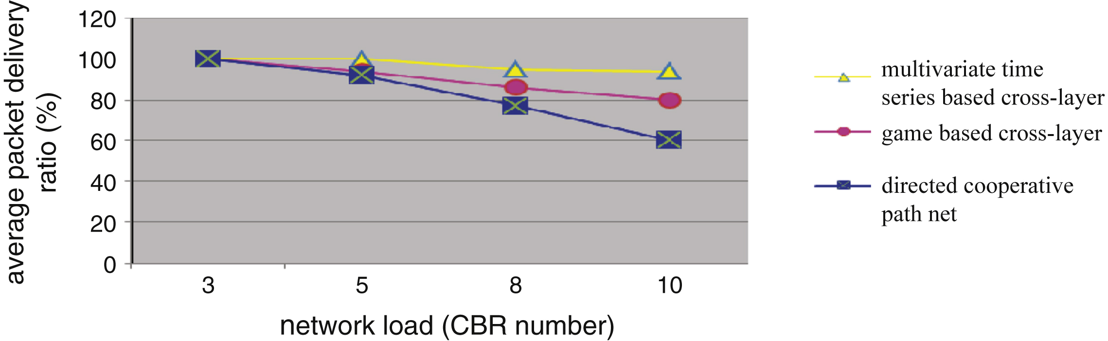
The proposed model prediction result is more accurate. Additionally, it has a linear time complexity and space complexity of O(n), whereas the AR model and many other time series models relate a time-consuming calculation of x n . A network processing mechanism of directed cooperative path net was proposed in [1], and a game theory-based cross-layer cooperation was proposed in [3]. We employ the average throughput and average packet delivery ratio to verify the congestion processing. Three congestion control mechanism results over an increasing network load are shown in Figs. 8 and 9. When the CBR number increases, the network’s throughput increases, and the average delivery rate decreases. Relative to the directed cooperative path net mechanism and the game theory-based cross-layer cooperation mechanism, the proposed mechanism realizes greater throughput as well as a lesser and flatter decline. This reveals that, with the prediction effect, the nodes in the directive cooperation path net have stronger adaptability.
5Conclusion
Aiming at improving network throughput and increasing the network packet delivery ratio, this paper combines the prediction method with the cross-layer design. Fuzzy time series prediction mechanism, which has a linear time complexity, extracts the cross-layered parameters of the average throughput and length of sending queue to forecast the network throughput situation. In addition, the directed cooperative path net is introduced to process the predicted congestion. Simulation, we verify the effectiveness of our optimization scheme. It is observed that the network throughput is effectively improved by the fuzzy time series-based congestion control, and the packet loss rate is reduced. Similarly, we can replace the average throughput with other cross-layer parameters to estimate the network congestion situation and verify the congestion control effectiveness. This will be included in our future work.
Acknowledgments
This research is partly supported by the National Nature Science Foundation of China under Grand no. 61272412, Ph.D. Programs Foundation of Ministry of Education of China no. 20120061110044, and Jilin Province Science and Technology Development program under Grant no. 20120303.
References
1 | Razaque A, Elleithy KM (2014) Energy-efficient boarder node medium access control protocol for wireless sensor networks Sensors 14: 3 5074 5117 |
2 | Cui C-S, Yang Y-J, Li X (2012) Research on congestion in wireless networks based on cross-layer design Advances in Information Sciences and Service Sciences 4: 20 552 561 |
3 | Zhang G-P (2011) Research on Game Based Wireless Resource Competition and Cooperation Mechanism China University of Mining and Technology Press Jiangsu Xuzhou |
4 | Li M-W, Jing Y-W, Li C-T (2013) A robust and efficient cross-layer optimal design wireless sensor networks Wireless Personal Communications 72: 4 1889 1902 |
5 | Han M, Liu X-X (2012) Stepwise input variable selection based on mutual information for multivariate forecasting Acta Automatica Sinica 38: 6 1000 1005 |
6 | Huynh T, Hwang WJ, Lee SH (2013) Throughput-optimal scheduling for cooperative communications in wireless ad hoc networks International Journal of Distributed SensorNetworks 2013: 3 286 291 |
7 | Duan W-X, Jiang W-X (2012) A congestion algorithm for wireless sensor networks based on ARMA traffic prediction Journal of Chinese Computer Systems 33: 005 1098 1103 |
8 | Chen Y, Qin F, Xing Y (2014) Cross-layer optimization scheme using cooperative diversity for reliable data transfer in wireless sensor networks International Journal of Distributed Sensor Networks 2014: 1 1 16 |
9 | Peng Y, Lei M, Li J-B (2014) A novel hybridization of echo state networks and multiplicative seasonal ARIMA model for mobile communication traffic series forecasting Neural Computing & Application 24: 3–4 883 890 |
10 | Lin Y-P, Yang Y-W (2010) Research on fuzzy time series model based stock market forecast Statistics and Decision 2010: 34 37 |
Figures and Tables
Fig.1
Fuzzy time series prediction flowchart.
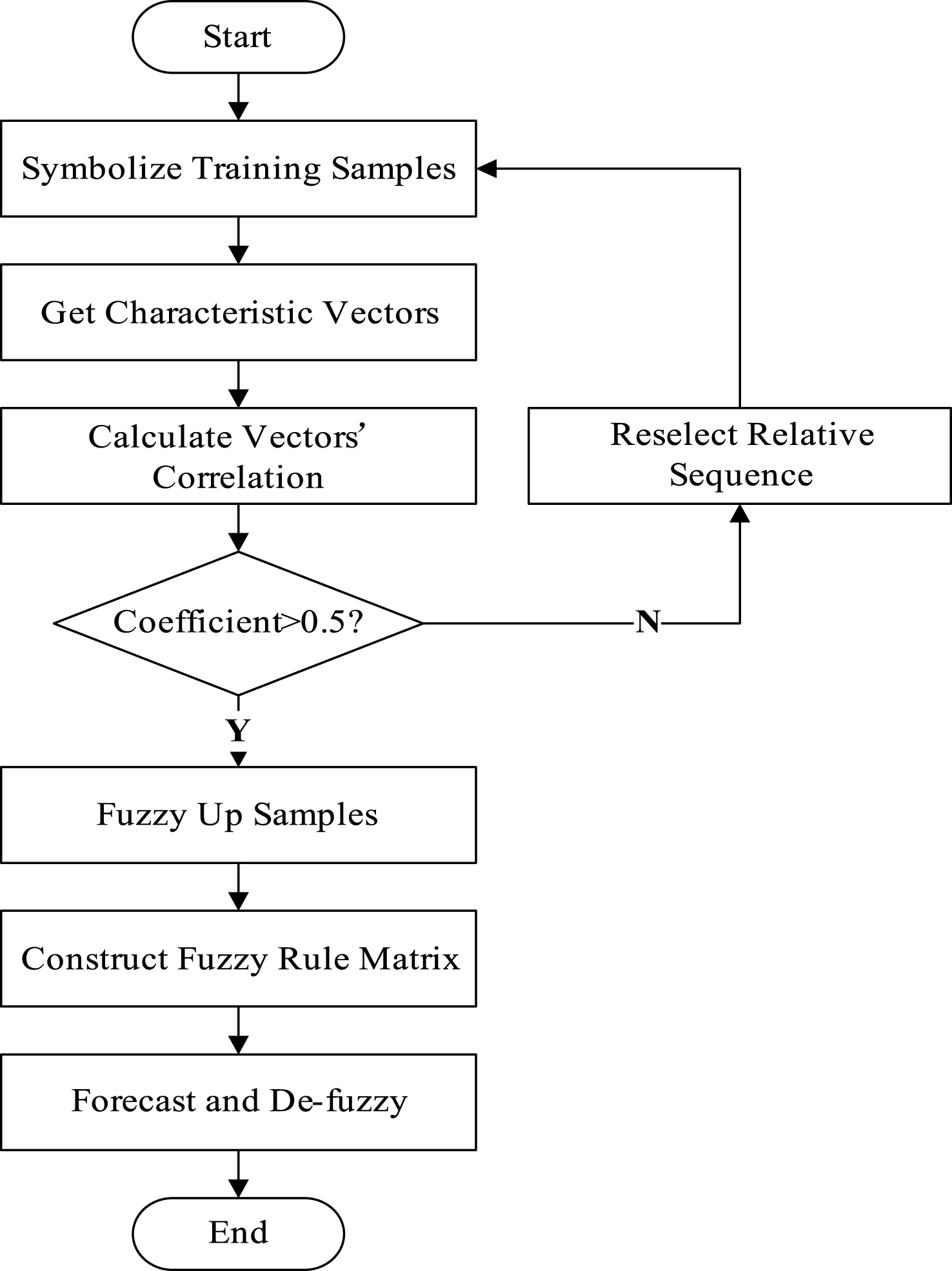
Fig.2
Multivariate time series prediction-based congestionprocessing flowchart.
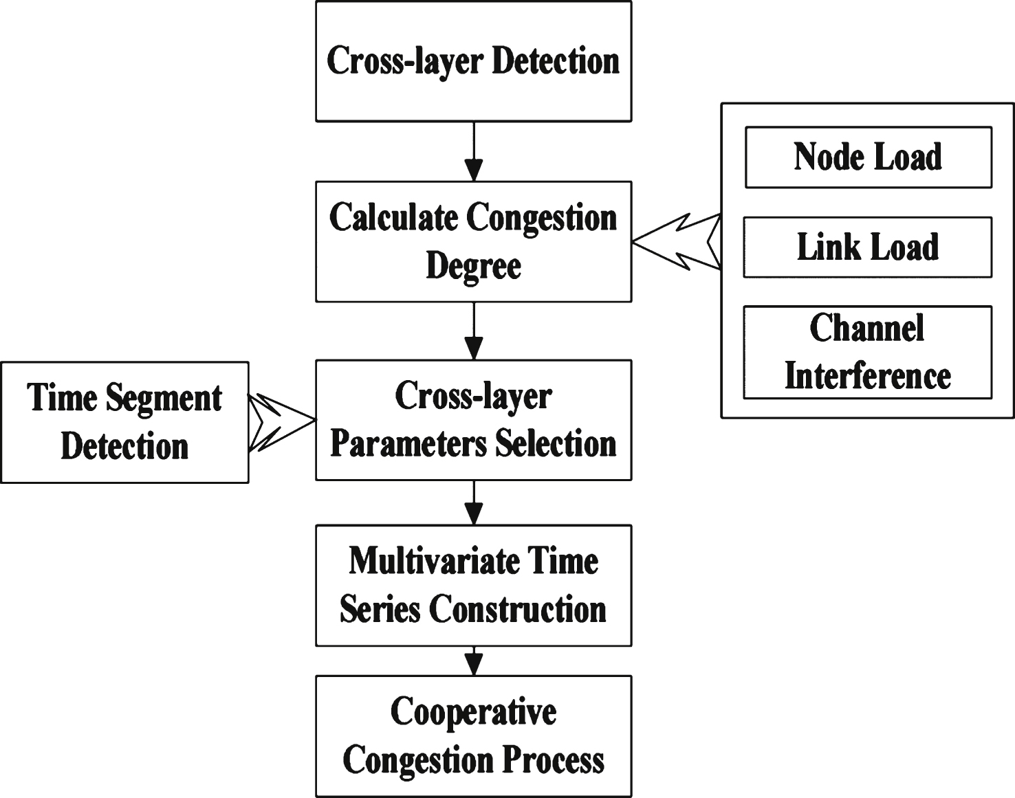
Fig.3
Schematic diagram of the directed cooperative path net.
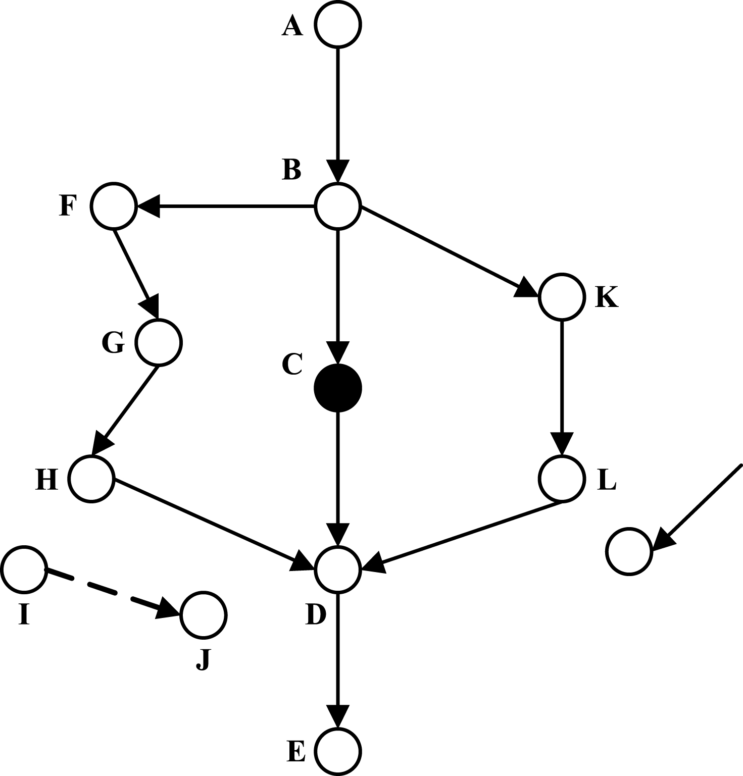
Fig.4
Simulation scene.
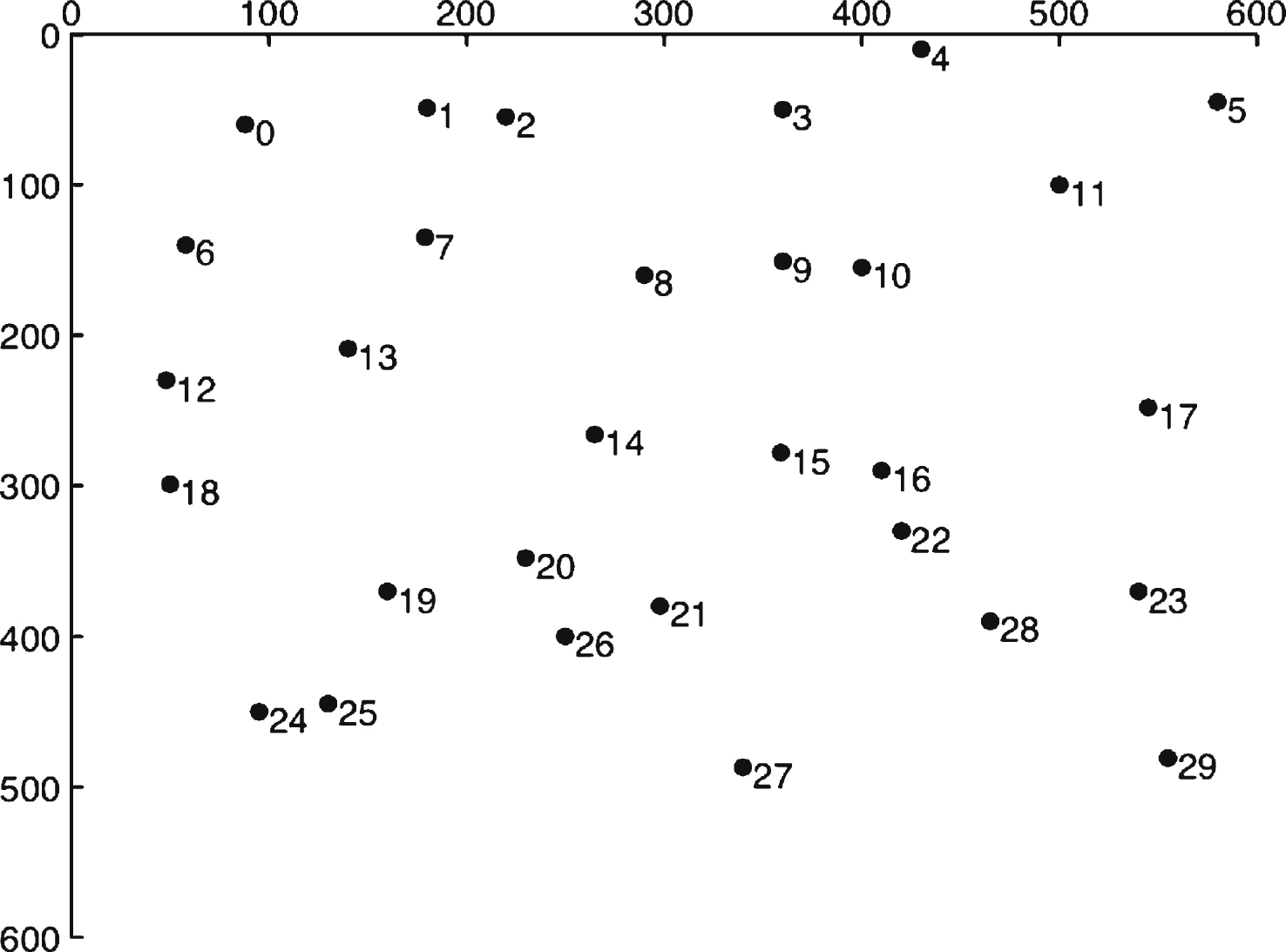
Fig.5
Two time series’ sequence diagram.
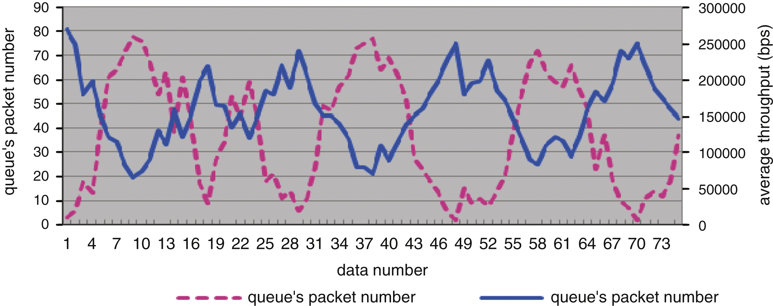
Fig.6
Average throughput prediction results.
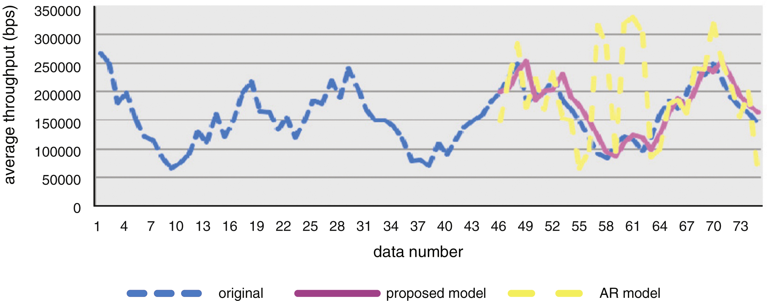
Fig.7
Telephone connection prediction and corresponding congestion rate.
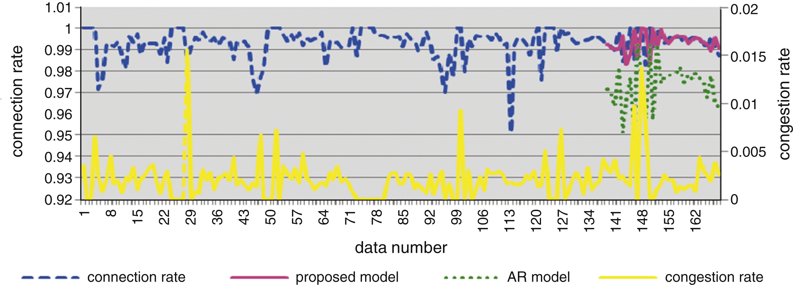
Fig.8
Wireless network overall throughput changing trends diagram.
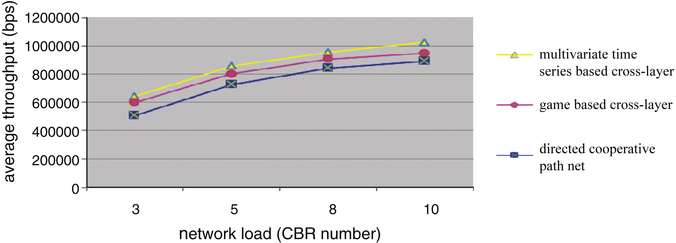
Fig.9
Average delivery rate changing trends diagram.