Crop region extraction of remote sensing images based on fuzzy ARTMAP and adaptive boost

Li, Da-Wei; Yang, Feng-Bao; Wang, Xiao-Xia

doi:10.3233/IFS-151983

Crop region extraction of remote sensing images based on fuzzy ARTMAP and adaptive boost

Issue title: The fuzzy system and its application in East Asia

Guest editors: Ildar Batyrshin, Dragan S. Pamučar, Paolo Crippa and Feng Liu

Article type: Research Article

Authors: Li, Da-Wei^{a; b; *} | Yang, Feng-Bao^a | Wang, Xiao-Xia^a

Affiliations: [a] School of Information and Communication Engineering, North University of China, Taiyuan Shanxi, P.R. China | [b] School of Computer and Control Engineering, North University of China, Taiyuan Shanxi, P.R. China

Correspondence: [*] Corresponding author. Da-Wei Li, Schoolof Computer and Control Engineering, North University of China, NO. 3 Xueyuan Road, Taiyuan Shanxi, 030051, P.R. China. Tel.: +86 13834522163; Fax: +86 351 3923623; [email protected]

Keywords: Remote sensing, corn region extraction, fuzzy ARTMAP, adaptive boost

DOI: 10.3233/IFS-151983

Journal: Journal of Intelligent & Fuzzy Systems, vol. 29, no. 6, pp. 2787-2794, 2015

Published: 2015

Get PDF

Abstract

Crop area statistics and yield prediction will affect adjustment of agricultural policy, to a certain extent. With the development of computer automatic classification techniques, the performance of classifiers are influenced by feature preprocessing and sample selection. Remote sensing classification according to spectral information is affected by false negatives and miscalculation in the complex spectrum area. Corn planting areas and other land-cover objects contain different surface structures and smoothness; other vegetation and villages have coarse textures. This paper introduces texture information based on a Gabor filter group to enrich land-cover information and establish a spectrum-texture feature set. With more samples, the algorithm efficiency is greatly affected. This paper proposes an improved fuzzy ARTMAP (FAM) with an adaptive boost strategy, namely Adaboost_FAM. Weak classifiers are trained to construct strong classifiers so as to improve operation efficiency. Meanwhile, classification accuracy will not be greatly improved. Experimental results indicate that the proposed method improves extraction accuracy when compared to classical algorithms, and improves efficiency when compared to algorithms which contain a great number of samples.

1Introduction

Agricultural remote sensing information extraction is one of the key technologies in remote sensing applications; many researchers have improved and explored various methods. Automatic classification accuracy and efficiency have been subjects of constant improvement. Anne Puissant proposes that texture information can greatly improve spatial resolution image classification [1]. However, single feature representation methods are unable to describe all relevant information, thus a multiple feature fusion method was developed. M. Fauvel used morphological properties to describe spatial information in order to combine spectrum characteristics [14]. This study overcomes the disadvantages of single feature classification and greatly improves the classification precision of the pixel scale. M. Fauvel and Y. Tarabalka combine morphological properties and multiple classifier methods to improve classification results, also demonstrating that texture and spectral information are important to image classification [15]. The texture of a corn field is different from that of villages and other vegetables, this feature has good consistency and regularity, therefore, this paper introduces texture information of corn areas to construct a multiple feature set and improve the accuracy of information extraction.

In general, remote sensing image classification methods can be divided into supervised classification and unsupervised classification methods. Unsupervised classification algorithms are those which do not account for prior knowledge, such as k-means and ISODATA. The disadvantage of these methods is that classification accuracy is low, resulting in rough classification results. Thus, these methods are not suitable for high resolution remote sensing images. Supervised classifiers include maximum likelihood [2], artificial neural networks, decision trees, support vector machines [13, 16, 17] and random forests. The key point is the selection of the test sample, because its quality is directly related to classification accuracy. Combination classification techniques include semi-supervised methods, and fusions of supervised and unsupervised methods.

Many new algorithms, such as the artificial neural network (ANN) [4, 6, 20], support vector machine (SVM) [18, 22, 24] and random forest [5, 7], meet the requirements of complex multispectral data. One of the most widely used methods for supervised classification in remote sensing analysis is the use of artificial neural networks (ANN), which are formed by algorithms inspired by biological neural systems. In an initial training stage, these networks fix coefficients between the input data and output categories. The process is completed by subsequent verification and test stages so that classification is determined to be correct or incorrect according to measures that were not involved in the test circumstances.

A supervised adaptive resonance theory (ART)-based neural network, namely fuzzy ARTMAP [10], is proposed as the base classifier. An incremental learning model is able to overcome the stability-plasticity dilemma of the data [8, 9]. The FAM network is plastic enough to absorb new information from new samples, and stable enough to retain previously learned information which may be corrupted by newly learned information. An interesting feature of FAM is that it integrates fuzzy set theory [12] and the stability-plasticity characteristic of ART into a common framework. Taherian and Arash proposed an efficient iris recognition system that employs a circular Hough transform technique to localize the iris region in the eye image and introduce a cumulative sum-based gray change analysis method to extract features from the normalized iris template. Then, fuzzy ARTMAP neural network was used to classify the iris codes [3]. Tan Shing Chiang introduced two models of evolutionary fuzzy ARTM-AP (FAM) neural networks to deal with imbalanced datasets in a semiconductor manufacturing operation [23]. However, these methods selected solitary samples, and thus did not account for diversity within samples, thus affecting the classification performance. This paper adopts ensemble learning, an adaptive boosting strategy, to develop fuzzy ARTMAP.

2Related research

2.1Fuzzy ARTMAP neural network

The Fuzzy ARTMAP network is composed of two types of fuzzy ART networks: ART_a and ART_b. One used training data and the other utilized verification data. The relationship between both fuzzy ART networks was determined by a memory map called map-field. The input data were normalized to 1 and duplicated by adding their complements. Thus, a data vector was obtained, which allowed the network weights and the maximum and minimum input values to be determined [11].

2.2Adaptive boost strategy

Adaptive boost strategy is an active learning method. Theoretical research proves that strong classifier error rates will be zero as long as each weak classifier classification error rate is below 50% and the number of weak classifier approaches ∞. In corn planting information extraction, in order to simplify the optimization of process parameters, it is necessary to construct weak classifiers based on few samples and brief characteristics. This mentality is feasible in theory. The algorithm is described as follows:

Step 1: Randomly select training data from the sample space group; initialize data distribution weights D _k (i) =1/m; initialize the parameters of the particle swarm optimization algorithm.

Step 2: When training the kth weak classifier, train SVM weak classifiers and predict output data based on training data and optimization parameters; then obtain prediction error of g (k) and e (k) = ∑_i D _k (i) i = 1, 2, …, m (g (k) ≠ y) where g (k) is the prediction result and y is the expectation result.

Step 3: Compute forecast sequence weight according to e (k):

(1)

α(k)=0.5ln(1-e(k)e(k))

Step 4: Adjust test data weight of the next iteration according to α (k):

(2)

Dk+1(i)=Dk(i)Bkexp[-α(k)yigk(i)] i=1,2,…,m

Step 5: Train K weak classifiers f (g _k, α _k) and construct a strong classifier:

(3)

h(x)=sign(∑k=1Kαkf(gk,αk))

3Experiment process and result

3.1Experiment datasets

Experiment data is derived from the fusion results based on a multi-spectrum image (B - G - R - NIR) and panchromatic image (pan); resolution is equal to 2 meters. To maintain consistent experimental conditions, this text selects three images from the same scene data in primary corn planting territory. Image sizes are 600 × 600, 1024 × 1024 and 400 × 400 pixels, respectively. Remote sensing images include corn, non-corn plants, and urban construction. Here, the corn crop planting area information extraction is studied; the corn area is identified as the area of interest, other areas are considered to be background. All experiments are conducted with a Windows 7 operation system with an Intel Core i5-2.30 GHz processor and 4.0 GB RAM.

3.2Feature extraction and selection

3.2.1Spectrum features

According to experience, NIR, R and G are selected as features. In addition, the common useful vegetation index (VI) contains the normalized differential vegetation index (NDVI), soil-adjusted vegetation index (SAVI) and enhanced vegetation index (EVI). The test selects three characteristics to obtain featuresets.

– NDVI is derived from red and NIR bands, and can effectively distinguish plants from otherobjects.

(4)

NDVI=NIR-RNIR+R

- SAVI can partially reduce the effect of a soil background. The modified soil-adjusted vegetation index (MSAVI) takes into account changes in soil factors without the soil index, and is suitable for areas of sparse vegetation coverage.
(5)
MSAVI=2NIR+1-(2NIR+1)2-8(NIR-R)2

(6)
SAVI=NIR-RNIR+R+L(1+L)

where L is the soil-adjusted index; values range from 0.5 to 1, and is equal to 0.5 in this paper.

– The effect of soil and atmosphere on NDVI are not independent; therefore, EVI simultaneously introduces feedback from two amendment regulations, using the soil adjustment index and atmospheric correction parameters.
(7)
EVI=NIR-RNIR+C1R-C2B+L(1+L)

where L is soil-adjusted index; values range from 0.5 to 1, and is equal to 0.5 in this paper. C ₁ and C ₂ are atmospheric correction parameters.

3.2.2Gabor filter texture features

These features are extracted by multi-scale and multi-orientation Gabor filters to simulate human vision in order to extract terse and concise contour information [25]. The feature extraction procedure is as follows:

Step 1: Extend Gabor filter g (x, y) to obtain a multi-scale and multi-orientation Gabor filter group by scale and rotation transformation.

(8)

g(x,y)=cos(2πf0x+φ)2πσxσye-(x2σx2+y2σy2)

where x, y are pixel positions; σ _x, σ _y are standard deviations of the Gaussian factors; f ₀ is the central frequency; and φ is the phase difference.

Step 2: Obtain a group of sub-images using the Gabor filter group.

(9)

fmn(x,y)=f(x,y)*gmn(x,y)

(10)

gmn(x,y)=a-mg(x′,y′), a>1

(11)

x′=a-m(xcosθ+ycosθ)

(12)

y′=a-m(-xcosθ+ycosθ)

(13)

θ=nπ/(n+1)

where a ^-m is scale factor of the mother Gabor wavelet; m is a scale number; n is of the orientation; and θ represents the filter orientation. This paper utilizes three scales and four orientations.

Step 3: Perform nonlinear transformation for each sub-image according to Equation (14).

(14)

Ψ(fmn(x,y))=1-exp[-2λfmn(x,y)]1+exp[-2λfmn(x,y)]

Step 4: Execute window operation for images of step 3.

(15)

Gt(x,y)=1Msxy∑(i,j)∈sxy|Ψ(fmn(i,j))|

Step 5: Compute average value of four orientations for each scale; then, obtain Gabor texture features.

3.2.3Features importance

Many studies show that the dimension of the feature vector greatly affects the algorithm efficiency. Although the vector dimension is not very large in this context, reducing the dimension of the feature set can improve the efficiency of the algorithm, which has practical

significance. This paper uses cross-validation to determine feature importance [19, 21], as shown in Fig. 1. According to experimental results, R, NIR, NDVI, homogeneity and contrast degree are selected to build a feature set. Although the degree of dimension reduction is small, it still affects the operational process. When the characteristic dimension is very large, this step has significant practical significance.

As shown in Fig. 1, the numbers of feature axle represent features B, G, R, NIR, NDVI, SAVI, EVI, and the Gabor texture of three scales, respectively. The spectral features are more important than textural features; this paper select G, R, NDVI, SAVI, EVI and the Gabor texture features of three scale degrees to execute subsequent supervised classification.

3.2.4Experiment results

This section implements experiments for three images, and compare results with those obtained by traditional classification methods. For the first experimental dataset, the number of samples and weak classifiers will affect the final classification performance, which is evaluated by the overall accuracy (OA) and Kappa coefficient. OA verifies the number of pixels that are classified correctly. Kappa can be used to assess the agreement of the two classifications for each class. This paper selects different numbers of samples. The results shown in Fig. 2 indicate that the classification performance can be improved with an increasing number of samples. Then, this paper selects different numbers of weak classifiers to construct Adaboost_FAM.

Figure 2 presents the Kappa sample curve, and the overall accuracy sample curve. Figure 3 presents the Kappa iteration curves, and the overall accuracy iteration curves.

(16)

Kappa=(TP+TN)M-(TP+FP)(TP+FN)+(TN+FN)(TN+FP)M2-(TP+FP)(TP+FN)+(TN+FN)(TN+FP)

(17)

OA=TP+TNM

(18)

M=TP+TN+FN+FP

where True Positive (TP) is defined as an entity labeled as “corn” that also corresponds to “corn” in the reference data. True Negative (TN) is an entity that belongs to “non-corn” in both the detection results and the reference data. False Positive (FP) is defined as an entity labeled as “corn” that corresponds to “non-corn” in the reference. False Negative (FN) is defined as an entity labeled as “nor-corn” that corresponds to “corn” in the reference. In view of the computational cost and precision, 1000 samples were randomly chosen to perform subsequent experiments. With the gradual increase of iterations, kappa and OA increase slightly but after 10 iterations, increase very slowly. Therefore in the subsequent process, classification indices based on above-mentioned parameters (1000 samples and 10 iterations) are compared to the indices obtained by classical classification methods. The classical methods contain Mahalanobis distance classification (Mahal Dist), Parallelepiped classification (Parallel), Maximum likelihood classification (Max Likeli) and Minimum distance classification (Mini Dist), and SVM. The comparison results are shown in Fig. 4 and Table 1.

Table 1 depicts the confusion matrix of classification and other indicators. Except for the kappa index and OA, the Producer Accuracy (PA) and User Accuracy (UA) metrics were computed using the following equations.

(19)

PA=TPTP+FN

(20)

UA=TPTP+FP

This paper utilizes fuzzy theory, neural networks and adaptive boost to construct a compound classification frame. The results of the proposed algorithm are markedly superior to results obtained by others. For the first remote sensing image with Adaboost_FAM (spectrum + texture), KAPPA, UA and OA are 0.5972, 0.7117 and 0.8532, respectively. SVM classification performance is similar to the proposed method, but the computational cost is too large due to parameter optimization.

To test the algorithm for image data which has a smaller or larger corn proportion, this paper selects two images as the analysis objects. For the second dataset, the performance indices are listed in Table 2. The KAPPA index, UA and OA are 0.698, 0.8461 and 0.8513, respectively; these values are superior to other traditional classifiers. The experiment demonstrates the effectiveness of the proposed method. The results of every method are shown in Fig. 5.

Classification precision parameters of the third dataset are listed in Table 3. In view of the terrain features of this experimental area in which the corn planting area is relatively small, after many experiments, the contribution of texture feature to the classification results is small. In some cases, it cannot even reach normal results. For the proposed method, KAPPA, UA and OA are 0.2489, 0.424 and 0.954, respectively. Due to the objective condition of the third dataset, the results are not superior to others. The non-corn area accounts for a large proportion of area; this masks the shortcoming of insufficient information to a certain extent.

4Conclusion

In the field of remote sensing classification, because of diversity and uncertainty of images data, same objects contain very different spectrum attributes, on the contrary, different objects may contain same spectrum attributes. According to the corn regional distribution characteristics, this paper introduces Gabor filter features to obtain a joint feature set. By applying fuzzy theory, neural network strategies, and adaptive boost strategy, a compound classification framework is implemented to extract the crop area. According to the experimental data, feature subsets and training samples were obtained. The work of this paper uses the adaptive boost strategy to optimize FAM classifiers, constructs weak classifier group which is based on less samples and simple feature set, gets Adaboost_FAM classifier, realizes information extraction process in shaanxi province. According to experimental results and analysis, the proposed method performs relatively well for the three studied datasets. Experiments indicate that classification precision is better than that obtained by typical supervised classification methods, as the parameter optimization and the training process takes less time than the traditional classification methods.

References

1	Puissant A, Hirsch J, Weber C (2005) The utility of texture analysis to improve per - pixel classification for high to very high spatial resolution imagery International Journal of Remote Sensing 26: 733 745
2	Shalaby A, Tateishi R (2007) Remote sensing and GIS for mapping and monitoring land cover and land-use changes in the northwestern coastal zone of Egypt Applied Geography 27: 28 41
3	Taherian A, Sh Mahdi A (2013) Noise resistant identification of human Iris patterns using fuzzy ARTMAP neural network International Journal of Security and its Applications 7: 105 118
4	Deilmai BR, Kanniah KD, Rasib AW, Ariffin A (2014) Comparison of pixel-based and artificial neural networks classification methods for detecting forest cover changes in Malaysia IOP Conf, Series: Earth and Environmental Science 18: 1 5
5	Jennifer C, Joseph MKF, Alisa GL (2013) Influence of multi-source and multi-temporal remotely sensed and ancillary data on the accuracy of random forest classification of wetlands in northern Minnesota Remote Sensing 5: 3212 3323
6	Yuksel C, Murvet K, Ece G (2014) Yield prediction of wheat in south-east region of Turkey by using artifi345 cial neural networks The 3rd International Conference on Agro-Geoinformatics Beijing, China
7	Hui F (2013) Land-cover mapping in the Nujiang Grand Canyon: Integrating spectral, textural, and topographic data in a random forest classifier International Journal of Remote Sensing 34: 7545 7567
8	Carpenter GA, Grossberg S (1987) A massively parallel architecture for a self-organizing neural pattern recognition machine Comput Vis Graph Image Process 37: 54 115
9	Carpenter GA, Grossberg S (1988) The ART of adaptive pattern recognition by a self-organizing neural network IEEE Comput 21: 77 88
10	Carpenter GA, Grossberg S, Markuzon N, Reynolds J, Rosen D (1992) Fuzzy ARTMAP: A neural network architecture for incremental supervised learning of analog multidimensional maps IEEE Trans Neural Netw 3: 698 713
11	Decanini JGMS, Tonelli-Neto MS, Malange FCV, Minussi CR (2011) Detection and classification of voltage disturbances using a Fuzzy-ARTMAP-wavelet network Electric Power Systems Research 81: 2057 2065
12	Zadeh LA (1965) Fuzzy sets Inform Control 8: 338 353
13	Dihkana M, Karslia F (2013) An SVM classifier and pattern-based accuracy assessment technique International Journal of Remote Sensing 34: 8549 8565
14	Fauvel M, Benediktsson JA, Chanussot J (2008) Spectral and spatial classification of hyperspectral data using SVMs and morphological profile IEEE Transaction on Geoscience and Remote Sensing 46: 3804 3814
15	Fauvel M, Tarabalka Y, Benediktsson JA (2013) Advances in spectral-spatial classification of hyperspectral images Proceedings of the IEEE 101: 652 675
16	Marconcini M, Camps-Valls G, Bruzzone L (2009) A composite isupervised SVM for classification of hyperspectral images IEEE Geoscience and Remote Sensing Letters 6: 234 238 sem
17	Pal M, Mather PM (2005) Support vector machines for classification in remote sensing International Journal of Remote Sensing 26: 1007 1011
18	Ujjwal M, Debasis C (2013) Learning with transductive SVM for semisupervised pixel classification of remote sensing imagery ISPRS Journal of Photogrammetry and Remote Sensing 77: 66 78
19	Poona NK, Ismail R (2013) Reducing hyperspectral data dimensionality using random forest based wrappers International Geoscience and Remote Sensing Symposium (IGARSS) Melbourne, VIC, Australia
20	Alessandro P, Valerio L (2014) Volcanic hot spot detection from optical multispectral remote sensing data using artificial neural networks Geophysical Journal International 196: 1525 1535
21	Luukka P (2010) Feature selection using fuzzy entropy measures with similarity classifier Expert Systems with Applications 38: 4600 4607
22	Swarnajyoti P, Lorenzo B (2012) A novel SOM-based active learning technique for classification of remote sensing images with SVM 32nd IEEE International Geoscience and Remote Sensing Symposium (IGARSS) 6879 6882 Munich, Germany
23	Tan SC, Watada JZ, Ibrahim Z, Khalid M (2015) Evolutionary fuzzy ARTMAP neural networks for classification of semiconductor defects IEEE Transactions on Neural Networks and Learning Systems 26: 933 950
24	Nicola S, Edoardo P, Farid M, Enrico B (2012) Local SVM approaches for fast and accurate classification of remote-sensing images International Journal of Remote Sensing 33: 6186 6201
25	Shang ZM, Lin ZR, Wen GJ, Yao N, Zhang CX, Zhang Q (2014) Aerial image clustering analysis based on genetic fuzzy C-means algorithm and Gabor-Gist descriptor 11th International Conference on Fuzzy Systems and Knowledge Discovery 77 81 Xiamen, China

Figures and Tables

Fig.1

Importance of each feature.

Fig.2

Classification performance indices with different number of samples. (a) kappa index; (b) overall accuracy.

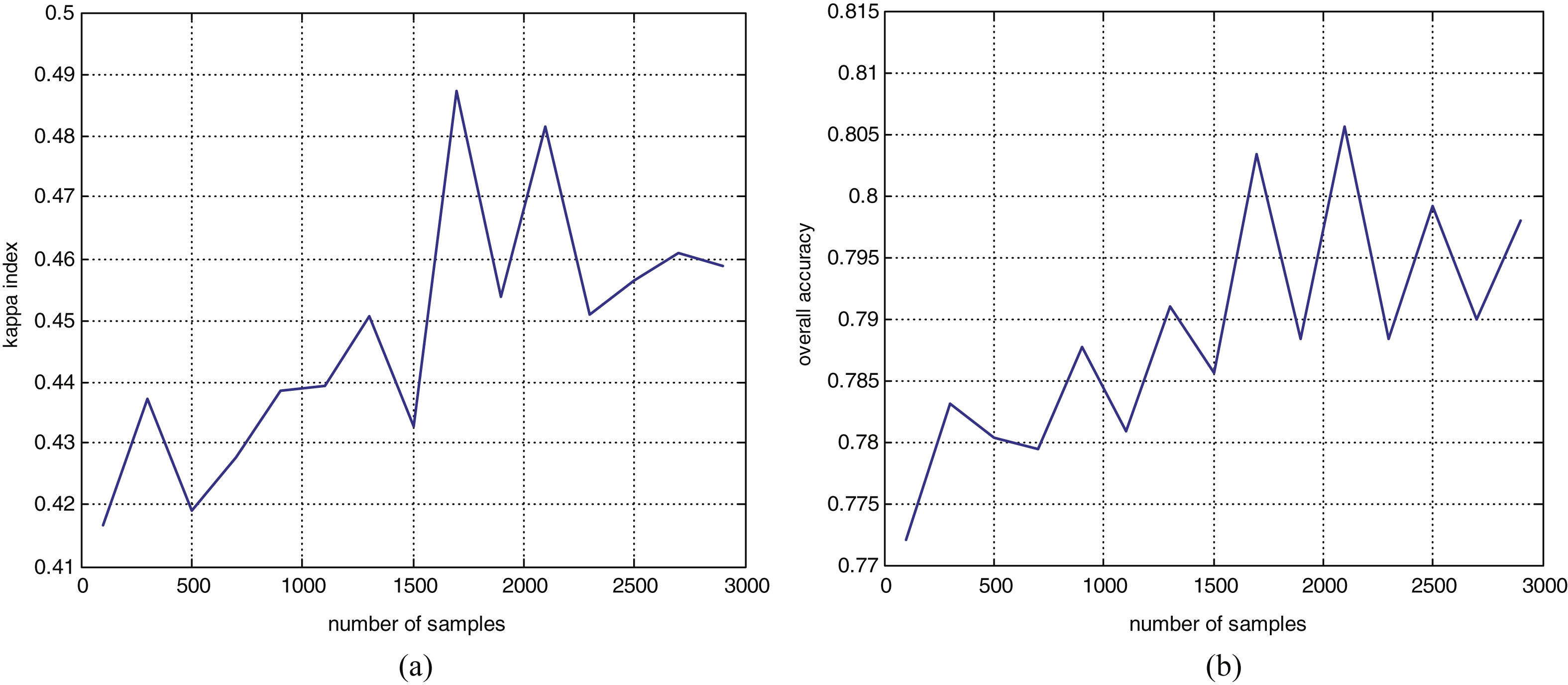
Fig.3

Classification performance indices with different numbers of iterations. (a) kappa index; (b) overall accuracy.

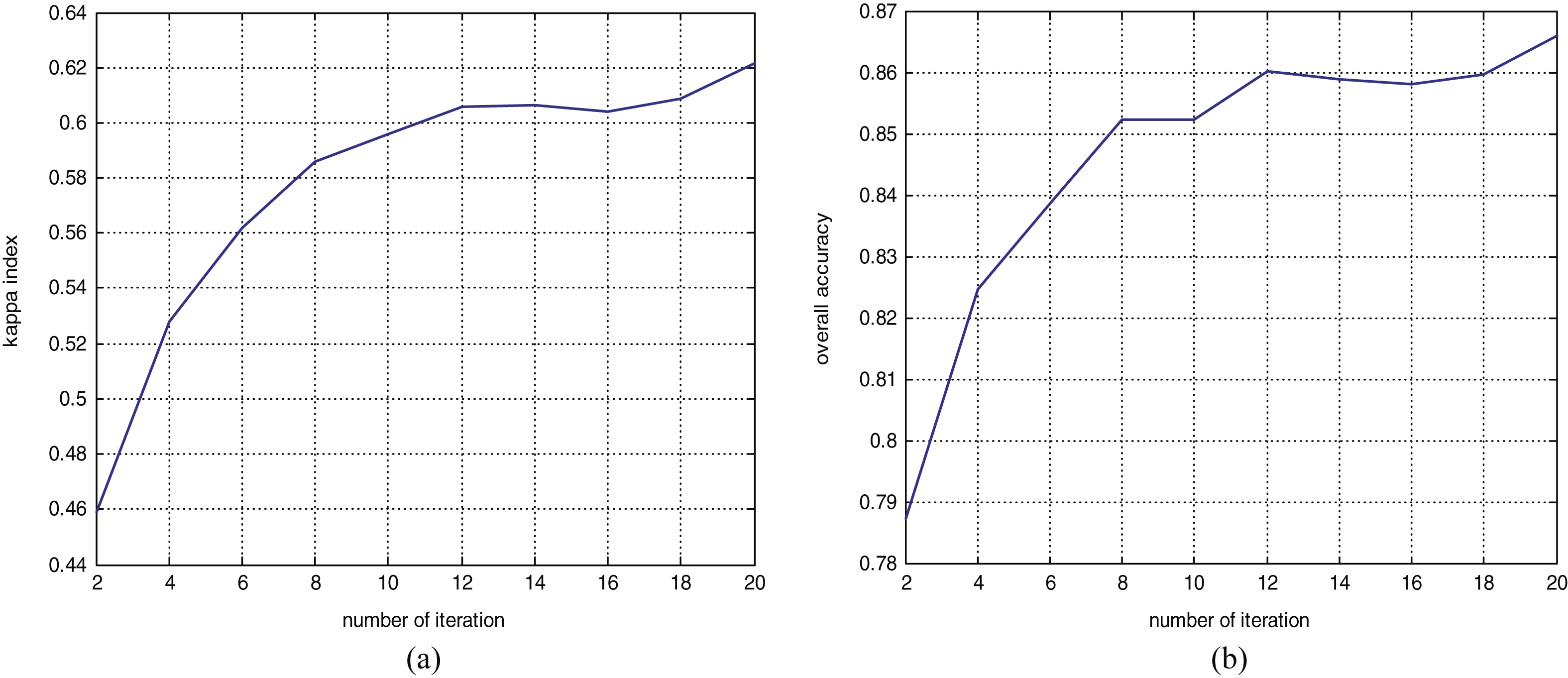
Fig.4

Classification results of the second dataset with different methods. (a) Ground truth; (b) Mahal Dist; (c) Parallel; (d) Max Likeli; (e) Mini Diste; (f) SVM; (g) Adaboost_FAM (spectrum); (h) Adaboost_FAM (texture); and (i) Adaboost_FAM (spectrum + texture).

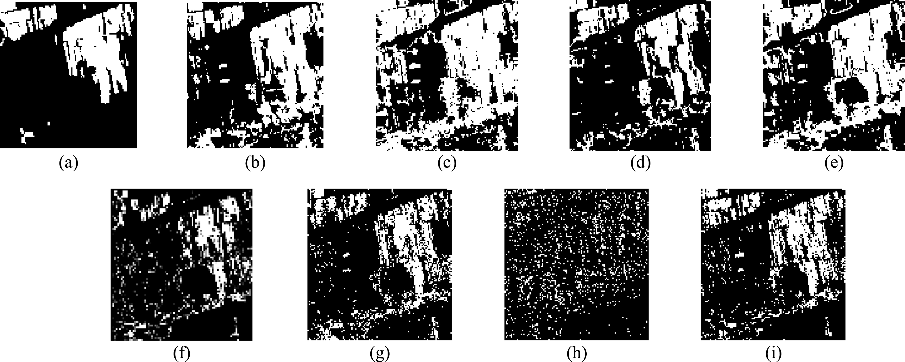
Fig.5

Classification results of the second dataset with different methods (a) Ground truth; (b) Mahal Dist; (c) Parallel; (d) Max Likeli; (e) Mini Diste; (f) SVM; (g) Adaboost_FAM (spectrum); (h) Adaboost_FAM (texture); and (i) Adaboost_FAM(spectrum + texture).

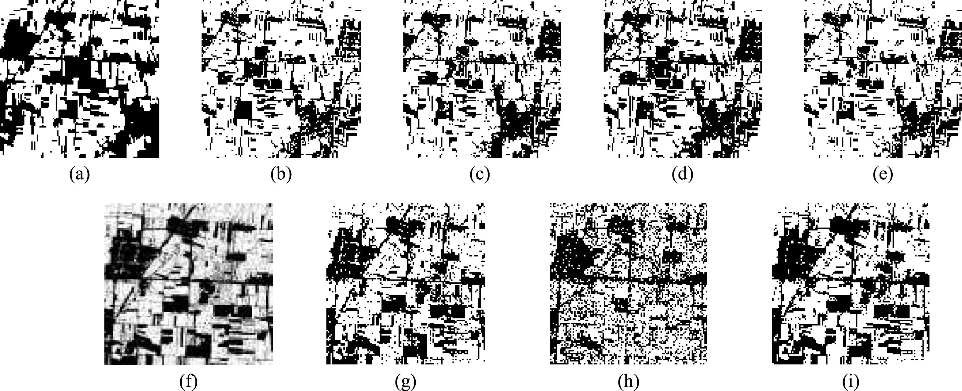
Table 1

Classification precision of the first dataset with different methods

Methods	TP	TN	FP	FN	KAPPA	UA	PA	OA
Mahal Dist	75738	212311	59228	12723	0.542	0.5612	0.8562	0.8001
Parallel	82314	168018	103521	6147	0.4006	0.4429	0.9305	0.6954
Max Likeli	62911	239212	32327	25550	0.5772	0.6606	0.7112	0.8392
Mini Dist	78288	195082	76457	10173	0.4817	0.5059	0.885	0.7594
SVM	50530	246296	25243	37931	0.5025	0.6668	0.5712	0.8245
Adaboost_FAM (spectrum)	55707	245306	26233	32754	0.5467	0.6799	0.6297	0.8361
Adaboost_FAM (texture)	17021	246015	25524	71440	0.1193	0.4001	0.1924	0.7307
Adaboost_FAM (spectrum + texture)	59850	247295	24244	28611	0.5972	0.7117	0.6766	0.8532

Table 2

Classification precision of the second dataset with different methods

Methods	TP	TN	FP	FN	KAPPA	UA	PA	OA
Mahal Dist	392946	161933	311417	182280	0.0258	0.5579	0.6831	0.5292
Parallel	379195	167809	305541	196031	0.014	0.5538	0.6592	0.5217
Max Likeli	347529	201586	271764	227697	0.0303	0.5612	0.6042	0.5237
Mini Dist	402027	143395	329955	173199	0.0019	0.5492	0.6989	0.5202
SVM	526830	328167	145183	48396	0.6203	0.7839	0.9158	0.8153
Adaboost_FAM (spectrum)	511159	359007	114343	64067	0.6532	0.8172	0.8886	0.8299
Adaboost_FAM (texture)	410595	303755	169595	164631	0.3558	0.7077	0.7138	0.6813
Adaboost_FAM (spectrum + texture)	512491	380162	93188	62735	0.698	0.8461	0.8909	0.8513

Table 3

Classification precision of the third dataset with different methods

Methods	TP	TN	FP	FN	KAPPA	UA	PA	OA
Mahal Dist	4859	136519	32303	2719	0.1571	0.1308	0.6412	0.8015
Parallel	4240	164352	4470	3338	0.4975	0.4868	0.5595	0.9557
Max Likeli	3883	162568	6254	3695	0.4093	0.3831	0.5124	0.9436
Mini Dist	4929	155960	12862	2649	0.3494	0.2771	0.6504	0.9121
SVM	2844	151112	17710	4734	0.1488	0.1384	0.3753	0.8728
Adaoost_FAM(spectrum + texture)	1496	166790	2032	6082	0.2489	0.424	0.1974	0.954